Séparation de niche entre deux espèces invasives de gobies

(1)

(2)

En vue de l’obtention du

DOCTORAT DE L’UNIVERSITÉ DE TOULOUSE Délivré par:

UNIVERSITÉ DE TOULOUSE III-PAUL SABATIER Présentée par:

Zhiqiang GUO

SÉPARATION DE NICHE ENTRE DEUX

ESPÉCES INVASIVES DE GOBIES

Co-dirigée par:

Prof. Jiashou LIU (Institute of Hydrobiology, CAS, China) Prof. Sovan LEK (Université de Paul Sabatier, France)

Dr. Julien CUCHEROUSSET (CNRS, France)

Jury

Prof. Josep LLORET (University of Girona, Spain) Rapporteur Prof. Boping HAN (Jinan University, China) Rapporteur Prof. Sovan LEK (Université de Paul Sabatier, France) Co-directeur Prof. Rodolphe GOZLAN (Institut de Recherche Pour le Développement, France) Examinateur Prof. Shouqi XIE (Institute of Hydrobiology, CAS, China) Examinateur Prof. Zhongjie LI (Institute of Hydrobiology, CAS, China) Examinateur

(3)

Acknowledgements

I would not have been able to finish my PhD research without the help and support of all the kind people around me, and thus to only some of whom it is possible to give particular thanks here.

Above all, the special appreciation goes to the two supervisors, Prof. Jiashou LIU and Prof. Sovan LEK, for their constructive suggestions and constant supports throughout my PhD study. Their excellent guidance, patience and financial support provide with me such a satisfying atmosphere for research. I owe my deepest gratitude to their care to my daily life (e.g. Prof. Jiashou LIU’s so much care when I stayed in hospital last year and Prof. Sovan LEK’s meticulous care when I study in Toulouse). I am a lucky dog to be a PhD student of the two. They have been a steady influence throughout my future life and research career.

I would like to express my sincere gratitude to Dr. Julien CUCHEROUSSET, the co-supervisor of my PhD thesis. His invaluable comments and conscientious works have contributed to the success of this research. I admire his perfect oral English like a native, high scientific standards, and extensive knowledge, etc. I have learned a lot from him and he has made such a good example for me on how to do research. I really appreciate for his kind helps in my daily life (e.g. driving me to see doctor on the weekend, filling the tables for registration, buying insurances, applying OFII, etc.)

I am greatly indebted to Prof. Zhongjie LI and Assoc. Prof. Tanglin ZHANG, who gave me many insightful suggestions on my PhD study. Thank them very much for generously sharing their knowledge and time, for being patient with my research. I wish to thank Prof. Youhe YU, Prof. Songguanx XIE and Dr. Shaowen YE whose constructive advises have substantially improved this work.

I owe my deepest gratitude to Assoc. Prof. Xiaoming ZHU and Prof. Shouqi XIE, for their constant guidance and care during my PhD study. When I was a beginner on research, their valuable suggestions, instructions and encouragement made me have more confidence. Thanks a lot for their important revision and comments on my manuscripts about sturgeons.

I would like to express a special appreciation to Assoc. Prof. Sithan LEK-ANG. Thank you so much for her astonishingly delicious foods and kindly looking after my life in Toulouse. Her and Prof. Sovan LEK entertained me so often that I feel Toulouse was my home town.

I am grateful of Dr. Thomas K. POOL for his careful and professional corrections of my manuscripts. His meticulous works significantly refined and improved those papers. I really learned a lot from him on how to adapt a new environment and join a new group as a new comer. I also own a particular gratitude to Ivan PAZ and Mathieu CHEVALIER for their perfect

(6)

I share the credit of this work with the teachers and colleagues at IHB (Mrs. Yunxia YANG, Dr. Wei LI, Dr. Ming DUAN, Dr. Dong HANG, Dr. Minglin LING, Dr. Fengyue ZHU, Dr. Jianfeng TANG,……..Mr. Xinnian CHENG, Mr. Guanghan NIE, etc.) and the members in Laboratory of Evolution, Diversity and Biology at UPS (Dr. Gaël GRENOUILLET, Prof. Sébastien BROSSE, Dr. Simon BLANCHET, Dr. Sebastien VIllÉGER, Dr. Loïc TUDESQUE, Dr. Lorenza CONTI, Dr. Christine LAUZERAL, Lise COMTE, Charlotte VEYSSIÈRE, Nicolas CHARPIN, etc.). To work with them has been a real pleasure to me.

I would like thank the Graduate Student Affairs Division of IHB (Mr. Xi FENG, Mrs. Kefeng LIU, Mrs. Mei ZHA and Mrs.Caipai LIAO) and the secretariat of EDB (Mrs. Linda JALABERT, Mrs. Nicole HOMMET and Mr. Frédéric MAGNÉ). I wish to thank Mrs. Dominique PANTALACCI for your generous helps with the registration, TOEIC test and so on.

Last and not the least, I sincerely thank my beloved wife, mum, dad and brothers. It is their whole-hearted support and endless love that made me to overcome all the difficulties through these years.

The research was financially supported by the National Natural Science Foundation of China (No. 31172387), the Major Science and Technology Program for Water Pollution Control and Treatment of China (No. 2012ZX07105-004), National S&T Supporting Program (No. 2012BAD25B08) and Program Cai Yuanpei 2011-2013 (Chinese Scholarship Council and University of Toulouse).

Faithfully yours Zhiqiang GUO Toulouse 29/10/2012

(7)

Résumé

Comprendre la coexistence d'espèces et le maintien de la biodiversitéest depuis longtemps un point central en écologie des communautés. La notion de niche, ou théorie des niches, a été largement développée depuis l’explication par Darwin de l’impressionnante diversité de la vie sur Terre. Celle-ci est considérée comme un mécanisme majeur permettant la coexistence d’espèces compétitrice au sein des communautés écologiques. La différenciation en niches spécifiques implique des différences spatiales, trophiques, temporelles et/ou une combinaison de celles-ci. Dans cette étude, la sélection d’habitat, les traits d’histoire de vie, la composition alimentaire et les comportements alimentaires de deux espèces invasives de gobiidés, très abondantes et écologiquement similaires (Rhinogobius cliffordpopei et Rhinogobius giurinus), sont comparées afin de tester si la séparation de niches est un mécanisme qui peut potentiellement permettre leur coexistence stable dans le lac Erhai (un lac superficiel d’eau douce du plateau de Yunnan-Guizhou en Chine).

Les résultats montrent qu’il y a séparation des niches de ces deux espèces le long d’un axe d’habitat, d’un axe alimentaire (pour l’habitat littoral et pour les adultes et sub-adultes), et d’un axe temporel (en termes de cycles de ponte).

Spécifiquement, R. giurinus occupe principalement les habitats profonds (PH) alors que R. cliffordpopei occupe principalement l’habitat littoral (LH). Des analyses corrélatives ont montré que l’abondance de R. giurinus est positivement associée avec la profondeur de l’eau et les substrats composés de sables limoneux et grossiers, tandis que la distribution de R. cliffordpopei est corrélée aux fortes densités en macrozooplankton, les fortes abondances en autres espèces de poissons, les fortes concentrations en oxygène dissout et les fortes densités en macrophytes submergées.

Concernant le partage en ressources alimentaires, les deux espèces ont montré de clairs changements au niveau de leur diète ontogénique ainsi que dans les patrons de partage des aliments qui sont significativement différents selon le stade de leur histoire de vie et les habitats.

(8)

consomment principalement des larves de Chironomidae et de Tubificidae.En LH, les sub-adultes et adultes des deux espèces présentent des différences significatives dans leur régime alimentaire alors que les juvéniles ont des régimes similaires. Cependant, en PH et SH, nous n'avons trouvé aucune preuve de partage des ressources alimentaires, quelque soit le stade de vie (juvéniles, sub-adultes et adultes).

R. cliffordpopei et R. giurinus présentent un partage de leur niche temporel. En effet, les deux espèces ont des débuts de période de reproduction ainsi que des pics de reproduction à des moments différents.R. cliffordpopei se reproduit de Février à Juin avec un pic de ponte entre Mars et Avril alors que l'activité de reproduction de R. giurinus se fait entre Avril et Août avec un pic de ponte pendant les mois de Mai et Juin. Ces différences ont conduit à un partage temporel des cohortes de taille similaire entre les deux espèces, en particulier pour les larves de petite taille et les juvéniles, qui sont presque exclusivement zooplanctivores et qui exploitent les mêmes ressources alimentaires dans le lac. Cependant, l'activité nycthémérale (activité de locomotion) et le rythme d'alimentation varient légèrement entre les deux espèces, i.e. les deux espèces présentent deux pics d'activités (6:00 - 10:00 et 18:00 - 22:00) et deux principales périodes d'alimentation (6:00 - 10:00 et 18:00 - 22:00) sur un laps de temps de 24h pour les quatre saisons.

De plus, notre étude apporte une compréhension complète de la sélection d'habitat et des traits d'histoire de vie (i.e. patron de croissance, biologie de la reproduction et dynamique de population) de ces deux espèces invasives de gobies. Ces résultats biologiques sont essentiels pour la mise en place de programmes économiquement et écologiquement efficaces de contrôle pour les deux espèces de ravageurs. De nouveau programmes de gestion sont fortement recommandés en vue de ces résultats. Par conséquent, dans cette étude, plusieurs programmes de

(9)

efficacité.

Mots clés: coexistence d'espèces, espèces de gobies, théorie des niche, séparation de niche, invasion écologique, gestion d'espèces invasives.

(10)

Understanding species coexistence and maintenance of biodiversity in nature has long been a central issue in community ecology. The niche or niche-based theory has been developed since Darwin’s explanation of an amazing diversity of life on the Earth and considered as a major theory explaining the coexistence among competing species within ecological communities. Niche differentiation basically involves spatial, trophic, temporal and/or a combination of them. In the present study, habitat selections, life characteristics, diet compositions and feeding behaviors of two highly abundant and ecologically similar invasive goby species (Rhinogobius cliffordpopei and Rhinogobius giurinus) are compared to test whether niche separation is a potential mechanism allow ing the stable coexistence of them in Lake Erhai (a shallow freshwater lake in the Yunnan-Guizhou Plateau of China).

The results demonstrated that these two species showed niche separation along habitat axis, food axis (in littoral habitat for sub-adults and adults), and temporal axis in terms of spawning cycles.

Specifically, R. giurinus mostly occupied profundal habitat (PH) while R. cliffordpopei mainly used littoral habitat (LH). Correlation analyses revealed that the abundance of R. giurinus was positively associated with deep water, silt and coarse sand substrata, whereas the distribution of R. cliffordpopei was positively associated with high densities of macrozooplanktons and high abundances of other fish species, high concentration of dissolved oxygen and high densities of submerged macrophytes.

For food resources partitioning, they showed a clear ontogenetic diet shifts and significantly different food partitioning patterns at different life stages and habitats. For both species, macrozooplanktons (Cladocera and Copepoda) were the main food for juveniles while sub-adults and adults primarily consumed Chironomidae larvae and Tubificidae. In LH, sub-adults and adults of the two species significantly

(11)

three life stages.

R. cliffordpopei and R. giurinus showed temporal niche partitioning as they exhibited different onsets of spawning and peaks of spawning seasons, and thus different growth and population dynamics, though both of them are short-lived species with a life span of about one year. R. cliffordpopei spawned from February to June with a spawning peak occurring in March and April. Spawning activity of R. giurinus occurred from April to August with a peak activity during May and June. These differences resulted in a temporal partitioning for similar-sized cohorts, especially for small-sized larvae and juveniles, which were almost exclusively zooplanktivorous and exploited the same food resources in the lake. Moreover, their different spawning cycles led to different peak seasons for the highest population density of the two species. However, the diel activity (locomotory activity) and feeding rhythm varied slightly between them, i.e. both species showed two peaks of activity (6:00 - 10:00 and 18:00 - 22:00) and two main feeding periods (6:00 - 10:00 and 18:00 - 22:00) in the four seasons.

Moreover, our study provides a full understanding of habitat selection and life characteristics (i.e. growth pattern, reproduction biology and population dynamic) of the two invasive gobies. These findings are crucial biological aspects for an economically and ecologically effective control programs to the two abundant pest species. The further management programs are highly recommended to give a careful consideration of these findings. Therefore, several specific remediation is suggested to improve the current management strategies from the perspective of cost-efficiency.

Key words: species coexistence, goby species, niche theory, niche separation, biological invasion, invasive species management

(12)

(13)

Introduction

1.1 Mechanism of species coexistence

A central question in community ecology is how to synthetically explain the observed patterns of species abundance in space and time, and across scales (Chesson, 2000; Hubbell, 2001; Amarasekare, 2003; Clark, 2009). The theoretical principle of competitive exclusion, also called Gause's law (Gause, 1934), predicts that one species would eventually outcompete and displace the other when they compete for the same critical resources within an environment. However, a striking pattern in nature is not to be the case in a large number of ecologically similar species. For instance, plant alpha diversity reaches astonishing levels in tropical forests (e.g. a single hectare of Amazonian forest can support more than 280 tree species Wright, (2002)). To obtain synthetic explanations for stable coexistence of species, several theories and hypotheses have been put forward, of which the two most influential ones are the “niche or niche-based theory” (Chesson 2000; Chase & Leibold, 2003; Silvertown, 2004) and the “unified neural theory” (Hubbell, 2001; Chave, 2004; Hubbell, 2005; Hubbell, 2006). These two concepts have sparked considerable controversy over more than two decades among ecologists (Gaston & Chown, 2005; Gewin, 2006; Adler et al., 2007; Clark, 2009).

The “niche or niche-based theory” (e.g. Lotka-Volterra competition model (Leigh, 1968); regeneration niche hypothesis (Grubb, 1977); storage effect (Caceres et al., 1997); resource ratio hypothesis (Tilman, 1982); microbial mediation hypothesis (Zobel et al., 1997); competition–colonization trade-off (Levine & Rees, 2002)) has dominated community ecology for nearly a century (Leibold, 1995; Chesson, 2000; Chase & Leibold, 2003). This theory assumes that every organism has a place or position to live in natural environment, in which there is a functional role of the living organism and a complex set of adaptations for propagatingtheir offspring (Grinnell, 1917; Rejmanek & Jenik, 1975). The ecological niche is a term describing the way of life of a species, i.e. how an organism and/or population

(14)

responds to various abiotic and biotic factors (e.g. resources, competitors, predators, parasites, pathogens, etc.) and how it, in turn, alters those factors (e.g. acting as a food source for predators and a consumer of prey, limiting access to resources by other organisms, etc. (Rejmanek & Jenik, 1975; Leibold, 1995)). Since many environmental factors may influence the living of a species in nature, Hutchinson (1957) took niche definition one step further by a quantitative formulation giving a full consideration of all the environmental factors. He viewed the fundamental niche of a species as an n-dimensional hyper-volume, in which the dimensions are environmental conditions and resources that define the requirements of an individual or a species (Hutchinson, 1957). Each of these different dimensions (i.e. a plot axis) of a niche represents a biotic or abiotic variable in the environment. Hutchinson's "niche" is the ecological space occupied by a species and also incorporates ecological "role" of the organisms, which may provides an actual snapshot of the “living” of a species in nature (Rejmanek & Jenik, 1975; Leibold, 1995; Kylafis & Loreau, 2011).

The niche concept was popularized by Hutchinson but ecologists have long intrigued why there are so many different types of organisms within a habitat as competitive exclusion principle (Gause, 1934) predicts that two species can mere occupy the same niche in the same environment for a long temporal (Chesson 2000; Silvertown, 2004). Thus, each species is thought to have a separate, unique niche across spatial and/or temporal scales, and the niche of a single species is the multivariate combination of environmental features within a particular set of abiotic and biotic conditions (Jones et al., 2001; Wright, 2002; Chase & Leibold, 2003). Subsequently, niche differentiation among species is suggested as a major mechanism of coexistence of species in ecological communities (Schoener, 1974; Ross 1986; Jones et al., 2001; Amarasekare, 2003; Kylafis & Loreau, 2011). The classic niche concept is a fundamental and central aspect of modern ecology, yet the understanding of the mechanisms of species coexistence has remained unclear by the

(15)

change only slowly over hundreds to millions of years (Wiens & Graham, 2005; Pearman et al., 2008).

Over the past two decades, Hubbell (2001) has developed the “unified neutral theory of biodiversity and biogeography” that has become a dominant part of biodiversity science and one of the concepts most often tested with field data and evaluated with models (Adler et al., 2007; Clark, 2009). This theory directly challenges the niche paradigm as it assumes that species are ecologically similar and equivalent with regards to the probabilities of birth, death, dispersal and speciation (Gaston & Chown, 2005; Gewin, 2006; Clark, 2009). It raises an extreme and provocative assumption that all individuals are ecologically identical, largely suggesting that niche differences are not needed to explain biodiversity patterns (Bell, 2001; Hubbell, 2005; Hubbell, 2006).

The neutrality originates from island biogeography and neutral theory of molecular evolution (random genetic drift). First, neutral assumption is that differences among species are proposed to have no substantial effect on biodiversity within a community, though individuals of certain species usually show some characteristics that make them look or function differently with other species (Bell, 2001; Hubbell, 2001). Second, the community is saturated, in which individuals are engaged in a zero-sum game whereby if one emigrates or dies another one will immigrate or be born to take its place. However, there is no influence of individual’s traits (e.g. life characteristics) over the contribution to community saturation because all important ecological aspects associated with those species are equivalent (Gaston & Chown, 2005). Random death, dispersal and speciation are the most important features in the neutral theory (Hubbell, 2001). Neutral theory predicts the possibility of highly diverse communities of equivalent species due to the assumption of fitness equivalence, which is, in fact, a stochastic or random process including birth, death, immigration, emigration and speciation. Thus, it is often described as a “dispersal-assembly” theory or a “stochastic” theory (Bell, 2001; Hubbell, 2006). Since all individuals are functionally equivalent and processes are neutrally driven

(16)

by random events, the coexistence of species is usually unstable in neutral communities (Chave et al., 2004).

Surprisingly, given its extreme simplification of a seemingly complex phenomena (i.e. species equivalence), the neutral theory has attracted enormous attention among ecologists and has successfully described the observed species–area relationships and species abundance distributions in several communities, especially in equatorial rainforests and coral reefs (Gewin, 2006). Those ecosystems are thought to be the best example of neutral dynamics because species are highly diverse with a limited potential to partition resources into niches. Niche theories, however, are hard to explain more generally in communities with many rare species and only a few abundant ones (Tilman, 2004; Gewin, 2006).

Over the last decades, the monograph “The Unified Neutral Theory of Biodiversity and Biogeography” (Hubbell, 2001) has provoked vigorous controversy among ecologists. The assumption that species are equivalent to each other in all important ecological aspects, which is far different from typical niche-based assumption that species are highly different from each other owing to the variations of niche requirements and “living” ability (e.g. ability for competition, exploitation resources and reproduction (Gewin, 2006; Leibold & McPeek, 2006; Clark, 2009)). The main disagreement of neutral theory is the extreme assumption of ecological or functional equivalence among all the species, which seems to completely ignore the differences in species-level traits such as habitat preferences, reproductive strategies physiological tolerances, dispersal abilities, etc. (Gaston & Chown, 2005). Another constraint of the neutral theory is that it only applies under some given circumstances and this makes it appropriate in such circumstances without a wider applicability. For instance, it primarily lies in attemptsto explain the high diversity of tree species in tropical forests or fishes in coral reefs,and particularly concerns trophically similar groups (Hubbell, 2001; Chave, 2004; Gaston & Chown, 2005). On the other hand, despite the fact that the niche theory has been long developed and

(17)

Chase & Leibold, 2003; Silvertown, 2004), it ignores the neutral process in nature (Gaston & Chown, 2005; Leibold & McPeek, 2006). At the very beginning, ecologists often treat niche theory and neutral theory as mutually exclusive explanations, but they now recognize that the controversy is, at the most, over the relative importance of niches and neutrality or unifying niche and neutral theories (Gaston & Chown, 2005;Leibold & McPeek, 2006; Adler et al., 2007). It is indeed a false for a dichotomy between niche and neutrality obscuring a fact that there are two processes simultaneously influencing the community of competing species (Tilman, 2004; Leibold & McPeek, 2006; Adler et al., 2007). Ironically, niche and neutral theory have reinvigorated each other as Gewin (2006) stated “the prevailing notion is that stochastic forces exist on one end of a continuum while deterministic forces occupy the other. Finding any truth that lies between is the challenge. It’s not niche or neutral…it’s determining the relative importance of the two”.

1.2 Niche theory

One of the most fundamental concept in modern community ecology is the ecological niche. Ecologists use niche concept to organize a general thought about the “living” ways of organisms in nature, in which organisms use resources, interact with each other, and assemble into communities or ecosystems (Leibold, 1995). The niche of a species is a result of evolutionary and natural selective processes, through which it fits itself into an ecological community or ecosystem by morphological, physiological, and behavioral adaptations (Tokeshi & Schmid, 2002; Nosil & Sandoval, 2008; Kylafis & Loreau, 2011). Therefore, ecological niche describes not only a physical position (i.e. habitat conditions necessary for persistence of the species) but also a functional role of a certain species in ecosystems. Niche is a very basic and fundamental ecological concept subsuming all of the interactions within a species and also the response to biotic and abiotic environments (Leibold, 1995).

The niche concept has been developed more than a century. The first attempt to describe the organism-environment relationships is the Darwin’s phrase “place in

(18)

natural economy” and Sencer’s term “correspondence” (Whittaker et al., 1973; Rejmanek & Jenik, 1975). Darwin (1859) refers to species “filling nearly the same place in the natural economy of the land” and to “a place in the natural polity of the country”. Darwin’s idea is the essence of the later united term "niche" in Grinnell (1917), Elton (1927), Hutchinson (1957) as well as other proponents (Rejmanek & Jenik, 1975).

Grinnell is generally acknowledged to be the first ecologist developing the ecological concept of the niche, though he is the not the first one using the word of “niche” (Whittaker et al., 1973; Leibold, 1995). In the typical paper “The niche-relationships of the California Thrasher” (Grinnell, 1917), he demonstrated that temperature was the main constraint on geographical range of thrashers. Moreover, he found that the dense bush crown was particularly important for thrashers to avoid predators. Therefore, those factors were defined to organize the niche of thrashers since they seemed to explain the thrasher’s distribution. Although Grinnell is interested in environmental factors (e.g. physical or climatic) that restrict a species’ potential geographical distribution, he makes greatly contribution towards the later development of niche theory whereby two fundamental thoughts, i.e. species originally evolve to fill their niches and no two species could have exactly the same niche (Grinnell, 1917).

Compared with Grinnell’s niche concept, the exciting progress by Charles Elton is related the niche of an organism to their food and enemies instead of the only sense of geographical distribution (Elton, 1927). Elton’s definition of niche, in fact, referred to an environmental “place” as well as ecological or functional role in its community. Elton made a great stride by incorporating the “role” to niche concept (Whittaker et al., 1973). A few years later, a central tenet of modern niche theory, “Gause’s principle” or “competitive exclusion principle”, was published by Georgii Frantsevich Gause (1934).

(19)

environmental factors as well as functional roles of a species in nature, and viewed the fundamental niche of a species as an n-dimensional hyper-volume. It is the first concept with a rigorous and quantitative formula of niche theory rather than the nebulous ones prior to Hutchinson (Whittaker et al., 1973; Rejmanek & Jenik, 1975). This formalization directly enables the measurement of the niche of an organism and also comparison of niches between two or more species. Moreover, Hutchinson recognized the “fundamental niche”, which is a full range of conditions (biotic and abiotic) and resources that could be used by a species completely free of any interference with other species under an ideal environment. The fundamental niche of a certain species is largely determined by heredity factors (e.g. life characteristics, feeding habits, morphological and physiological limitations). In real word, however, there is a large number of external constraints (e.g. competitor, predation, etc.) limiting the breadth of the fundamental niche. A subset of the abstract fundamental niche under the presence of all interactions with other species is termed the “realized niche”, which is usually narrower than the fundamental one (Hutchinson, 1957).

As formulated by Hutchinson, the niche of a species involves each of the all dimensions (abiotic and biotic) as well as a combination of them, and/or the interactions among different species within communities (Hutchinson, 1957; Kylafis & Loreau, 2011). In practice, however, describing the niche of a species is often a bit difficult due to potentially infinite dimensions. Thus it may be hard to find the significant niche axes of the species without a good understanding of its biology and ecology. Consequently, few intergrative variables may ofen be sufficient to separate species’ realized niches among ecologically similar or competing species within communities. These variables are habitat segregation, food resources specialization and/or temporal differentiation (Chesson, 2000; Tokeshi & Schmid, 2002; Kronfeld-Schor & Dayan 2003; Nosil & Sandoval, 2008).

(20)

1.3 Niche differentiation

In heterogeneous environments, niche differentiation (synonymous with niche segregation, niche separation or niche partitioning) has long been considered as a major mechanism allowing the maintenance of biodiversity at different scales (Chesson 2000; Chase & Leibold 2003; Leibold & McPeek, 2006). For stable coexistence in competition models, species must differ their responds to, and/or effects on, the environment, including resources they share and all other factors that potentially influence population growth and fitness (Chase & Leibold, 2003). The limiting similarity in Hutchinson’s niche model also predicts that the realized niche of certain species is exclusively compared with the others within communities. There is no complete overlap in the realized niches between species and two species can mere share a single realized niche in a stable environment use (Hutchinson, 1957). However, proportional overlap in realized niche is possible, i.e. species may not differ at trophic resources but can differ at microhabitat (Chesson, 2000; Amarasekare, 2003). Therefore, species with little niche overlap along one or two axes can probably allow a long-term coexistence, but somewhat larger overlap can not.

Coexistence among competing species can be certainly maintained by niche separation, but how niche differentiation arises among closely related species is poorly know now? Interspecific competition is widely viewed to be one of the main forces driving a separation in ecological niches to limit niche overlap (Tokeshi & Schmid, 2002; Kylafis & Loreau, 2011). Niche differentiation can arise from current competition (The Ghost of Competition Present), past extinctions (The Ghost of Competition Past) and evolving differences (Morris, 1999; Tilman, 2004; Nosil & Sandoval, 2008; Miller et al., 2009). These competition processes eventually result in niche separation and resources partitioning between competing species in a local community, and thus allowing long-term coexistence (Chesson, 2000; Chase & Leibold, 2003).

(21)

differentiation involves a very large number of possible abiotic and/or biotic factors, of which the three basic dimensions are spatial (i.e. species may differ in terms of where they experience and respond to limiting factors), trophic (i.e. species can differ in terms of what they exploit from the same environment), temporal (i.e. species can differ in terms of when they respond to the same limiting factors or exploit the same resources) and/or a combination of them (Schoener, 1974; Ross, 1986; Jones et al., 2001; Amarasekare, 2003; Kronfeld-Schor & Dayan, 2003; Leibold & McPeek, 2006). Generally, habitat dimension is more important than the trophic dimension and then the temporal dimension (Schoener, 1974). However, Ross (1986) reviewed the resource partitioning patterns among seven global habitats (tropical reefs, temperate reefs, coastal marine, the Antarctic, mesopelagic/slope environments and freshwater streams and lakes) and concluded that, unlike in terrestrial systems, trophic separation is more important than habitat separation in fish assemblages. Among 37 studies that concurrently examined the niche differentiation along spatial, tropic and temporal axes, he found that about 57% niche showed the greatest separation along food, 32% along habitat, and 11% along time (Ross, 1986).

Nature is strikingly patchy in space and there is always a significant level of spatial heterogeneity in species distribution and abundance (Chesson, 2000; Jones et al., 2001). Organisms that live in different habitats or microhabitats have no direct or indirect interactions with each other and they can coexist stably for a long term even if they may share the same niche (Schoener, 1974; Ross, 1986; Chesson, 2000). Environmental heterogeneity in space is, therefore, a sufficient condition for discreteness of ecological niches. Niche differentiation along space (i.e. habitat segregation) has often been implicated as one of primary mechanism for coexistence among sympatric species with niche overlap (Chesson, 2000; Nicastro et al., 2010). Several studies on taxonomically related or ecologically similar aquatic species have contributed substantially to our understanding the role of spatial segregation in resources partitioning and communities structuring (Cooper et al., 2008; Hernaman &

(22)

Probert, 2008; Nicastro et al., 2010). Moreover, as diet compositions of a consumer have substantial implications not only for its biology but also for its impacts on sympatric species and community structure, niche differentiation along food resources (i.e. trophic niche segregation) plays an important role in promoting ecological differentiation and maintaining species diversity (Chesson, 2000; Kylafis & Loreau, 2011). Although theory suggests that niche differentiation along temporal (i.e. temporal partitioning) also be an important strategy mediating ecological interactions and facilitating coexistence among co-occurring competitors, its role in structuring communities has often been overlooked (Kronfeld-Schor et al., 2001; Kronfeld-Schor & Dayan, 2003). However, a growing number of studies have accumulated and provided empirical evidences of temporal partitioning between competing species such as ants (Albrecht & Gotelli, 2001), bats (Adams & Thibault, 2006), mice (Jones et al., 2001; Gutman & Dayan, 2005) and birds (Veen et al., 2010). In fish assemblages, however, the role of the niche separation along temporal axis has received less attention (Alanärä et al., 2001).

1.4 Ecological invasion of goby species

Invasive species are one of the greatest threats to global biodiversity (Butchart et al., 2010; Vörösmarty et al., 2010) and the impacts of invasive specie are especially widespread in freshwater ecosystems that are particularly vulnerable to biological invasions (Vörösmarty et al., 2010; Cucherousset & Olden, 2011). Fishes are among the most widely introduced group of aquatic animals and the 10 most frequently introduced aquatic species are all freshwater fishes (García-Berthou et al., 2005; Gozlan, 2008). The overall number of introduced fishes worldwide from known sources reaches 624 and the rate of non-native freshwater fishes introduced has doubled in the past 30 years (Gozlan, 2008; Gozlan et al., 2010). Since many invasive fishes have significant ecological, evolutionary and/or economic impacts on

(23)

(i.e. hybridization and introgression), alteration of recipient ecosystems, and dissemination of pathogens (Cucherousset & Olden, 2011; Gozlan et al., 2010).

Gobiidae is one of the largest families of fishes with more than 2000 species. Many goby species have been widely introduced and become established out of their native ranges including in North American (Dillon & Stepien, 2001; Copp et al., 2005), in Europe (Copp et al., 2005) and in Asia (Du et al., 2001, Yuan et al., 2010). In the Great Lakes, for instance, several goby species native to the Ponto-Caspian area have spread to all five lakes, notably the round goby Apollonia melanostoma (Pallas, 1814), the tubenose goby Proterorhinus semilunaris (Heckel, 1837) and the racer goby Neogobius gymnotrachelus (Kessler, 1857) (Dillon & Stepien, 2001). In European, some goby species have also invaded new areas and continue to establish new populations, including the round goby, the bighead goby Neogobius Kessleri (Günther, 1861), the monkey goby Neogobius fluviatilis (Pallas, 1814) and the racer goby (Copp et al., 2005). In Asia, freshwater gobies of the genus Rhinogobius (Gill 1859) are frequent benthic fish fauna in most East Asia countries, including China, Korea, Japan and some other regions of south-eastern Asia, such as Philippines, Vietnam and Thailand (Chen & Shao, 1996; Sone et al., 2001; Wu & Zhong, 2008). There are at least 17 nominal species of Rhinogobius in China (Wu & Zhong, 2008). The introduced gobies of genus Rhinogobius have established in most lakes of Yunnan-Guizhou Plateau (Xie et al., 2001, Yuan et al., 2010). The rapid proliferation of these species has raised serious concerns over their long-term negative impacts on native species and ecosystems (Xie et al., 2001; Cooper et al., 2008; Yuan et al., 2010; Kornis et al., 2012). The most notorious species is the round goby, one of the most wide-ranging invasive fish on earth, which has widely introduced into Laurentian Great Lakes watershed, the Baltic Sea and several major European rivers and has showed many nagetive effects on ecosystems (Kornis et al., 2012). The invasive round goby affects many native species through resource competition, spawning interference and displacement of native species to sub-optimal habitat (Kornis et al., 2012). In the Great Lakes, it has resulted in several ecological effects

(24)

such as alteration of nutrient and contaminant pathways, and increasing outbreaks of avian botulism (Ng et al., 2008; Kornis et al., 2012). However, few studies have paid attention to specific management strategies for the invasive goby species (Gozlan et al., 2010; Kornis et al., 2012).

Because of the wide and significant ecological and economic impacts of no-native fishes on recipient ecosystems (many of those impacts are detrimental), an increasing attention has been devoted to the management of invasive fishes (e.g. preventing their further invasion, mitigating their negative ecological effects, etc.) during the last decade (Sutherland et al., 2009; Gozlan et al., 2010). Several measures (e.g. physical removal, chemical eradication and bio-manipulation) have been developed and implemented to control, contain or eradicate a wide range of invasive species (Taylor & Hastings, 2004; Britton et al., 2011). The effectiveness of these measures is, however, highly dependent upon the life, biological and ecological characteristics of the targeted invasive species (Ludgate & Closs, 2003; Taylor & Hastings, 2004; Britton et al., 2011; Yeates et al., 2012). For instance, the egg of Salmonids are around 100 times less sensitive to rotenone than juvenile and adult (Marking & Bills, 1976), and therefore eradications using rotenone should account for different vulnerabilities among life stages (Ling, 2002; Britton et al., 2011). Therefore, a full understanding of the life characteristics of invasive species is crucial to develop economically and/or ecologically effective management strategies (Ludgate & Closs, 2003; Taylor & Hastings, 2004; Yeates et al., 2012).

Watersheds of the Yunnan Province is one of the highest biodiversity hotspots in China and there are 432 documented freshwater fish species, accounting for 42.2% of the total freshwater fish species of China (Xie et al., 2001). However, many invasive fish species have been introduced since the 1950-60s and a large number of native fish species (about one third of 432 native fish species) have become endangered or extinct (Xie et al., 2001; Yuan et al., 2010). For instance, seventeen native fish species inhabited in Lake Erhai in the 1950s (Du & Li, 2001).

(25)

species. The most notorious introduced fish species in lakes of the Yunnan Province are small-bodied goby of the genus Rhinogobius (Gill 1859) and Neosalanx taihuensis (Chen, 1956), Pseudorasbora parva (Temminck & Schlegel, 1846), Hypseleotris swinhonis (Günther, 1873), Hemiculter leucisculus (Basilewsky, 1855) and Abbottina rivularis (Basilewsky, 1855) (Yuan et al., 2010). Although significant attention has been paid locally to these species, the control actions have minimal success or require indefinite investments and the outcomes are often discouraging (Du & Li, 2001; Yuan et al., 2010). An important fact overlooked here was that most of these management strategies were implemented without an appropriate knowledge of life, biological and ecological characteristics.

1.5 Specific objectives

Rhinogobius giurinus (Rutter, 1897) and Rhinogobius cliffordpopei (Nichols, 1925) are frequent species (native species) in lakes along the middle and lower reaches of the Yangtze River (Xie et al., 2000a; Xie et al., 2005; Zhang, 2005; Li et al., 2010). They were inadvertently introduced into most lakes of the Yunnan-Guizhou Plateau in the 1950-60s and introduced simultaneously to Lake Erhai in 1961 (Du & Li, 2001; Xie et al., 2001; Yuan et al., 2010). Since then they have become the most dominant benthic fish species with the annual yield accounting for 48 % of total fish yields (kg) of the lake in 2010 (unpublished data). In native lakes along the middle and lower reaches of the Yangtze River, they are ecologically similar species with comparable life histories, such as small-sized (maximal total body length < 80 mm), reproducing in spring and early summer, zooplanktivorous, etc. (Xie et al., 2000a; Xie et al., 2005; Zhang, 2005). The present study focuses on the mechanisms that allow a long-term coexistence of two congeneric and competing goby species within this lake. Consequently, habitat selections, life characteristics, diet compositions and feeding behaviors of the two highly abundant and ecologically similar invasive goby species (Rhinogobius cliffordpopei and Rhinogobius giurinus) were compared to test

(26)

whether there was a niche separation (involving spatial, trophic and temporal axes) allowing their stable coexistence in the lake.

Specifically, in the study of habitat selections (i.e. niche separation along spatial axis), the objectives were to determine whether spatial segregation occurs between the two species by examining how their abundances differed across the habitats and how their abundances were associated with environmental characteristics. In the study of food resources exploitation (i.e. niche separation along trophic axis), our aims were to determine whether the trophic niche (food resources) of the two species differed in each habitat and how their trophic niche changed with habitats as well as life stages during ontogeny. In the study of life characteristics (age, growth, reproduction biology and population dynamic) and feeding behaviors, our objectives were to investigate temporal partitioning (i.e. niche separation along temporal axis) in terms of spawning cycles, appearance of similar-sized cohorts, population dynamics, diel activities and feeding rhythms.

Moreover, the two species mainly prey on large zooplankton (Cladocera and Copepoda) and aquatic insects (Chironomid larvae), and they often prey on fish larvae and eggs, including those of native species (Xie et al., 2000a; Du et al., 2001; Zhang, 2005). They are widely considered to compete with native species (e.g. Cyprinus longipectoralis (Chen & Huang, 1977), Cyprinus barbatus (Chen & Huang, 1977), Barbodes daliensis (Wu & Lin, 1977)) for food resources (Du et al., 2001) and reduce the native species especially when their populations are highly abundant in the lake. The two species are therefore thought to be one of the major causes of the decline and/or extinction of most native fishes in the lake (Du et al., 2001). Currently, the principal management strategy to control the two species in the lake is the removal by the local fishery, but the outcomes are discouraged as the populations of those two gobies have become more dominant in the latest years. Thus, based on their habitat selections and life characteristics (i.e. growth pattern, reproduction biology and population dynamic), this study aimed at providing

(27)

specific strategies to improve the cost-efficiency of the current management programs for the two pest species.

(28)

2 Materials and Methods

2.1 Study site and habitat characteristics

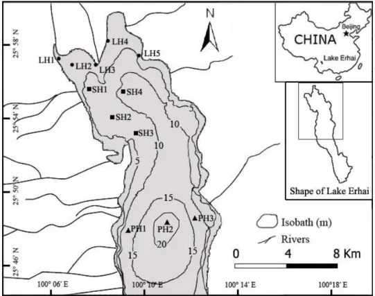
Lake Erhai (105°5-17′ E, 23°35-58′ N) is a freshwater plateau lake in Yunnan-Guizhou Plateau of China (Fig. 1). Its surface area is about 250 km2 and catchment area is about 2,600 km2. The maximum water depth is approximately 21 m without thermal or dissolved oxygen stratification. Water temperature usually peaks at around 25-27 °C in July or August and drops to approximately 6 - 8 °C in December or January. Currently, twenty-eight fish species have been found in the lake in recent years and most of them are planktivorous. The dominant species are small-bodied fishes, especially non-native species, including freshwater gobies Rhinogobius giurinus and R. cliffordpopei, Neosalanx taihuensis (Chen, 1956), Pseudorasbora parva (Temminck & Schlegel, 1846), Hypseleotris swinhonis (Günther, 1873) and Hemiculter leucisculus (Basilewsky, 1855). Channa argus (Cantor, 1842) is the only recorded piscivorous fish species.

Fig. 1 Sampling sites in the three habitats located in the central and northern section of Lake Erhai

(29)

Habitat characteristics of the lake were investigated prior to fish sampling in 2010 (Table 1). Habitats for benthic fishes in Lake Erhai were classified into three types: 1) littoral habitat (LH, water depth less than 6 m, high abundance of submerged macrophytes, submersed-macrophyte detritus substrata); 2) sub-littoral habitat (SH, water depths range 6 to 12 m, few submerged macrophytes, submersed-macrophyte detritus and silt substrata); and 3) profundal habitat (PH, water depths ranges 12 to 20 m, no submerged macrophytes, silt and coarse sand substrata, Fig. 1 & Table 1). There were Five (LH1-LH5), four (SH1-SH4) and three (PH1-PH3) sites in each habiat (Fig. 1 & Table 1). For each sampling site, water temperature, dissolved oxygen and conductivity were measured in situ using a handheld meter (YSI Model Pro20, Ohio, USA). A handheld pH meter was used to measure pH in situ (YSI Model EcoSense pH10A, Ohio, USA). Total nitrogen, total phosphorus and Chlorophyll a were determined using a standard colorimetric method (APHA et al., 1995). Macrozooplanktons were collected by hand-nets (mesh size 64 μm) and counted under a dissecting microscope. Substrata structures were sampled by Peterson dredge (0.0625 m2) and determined by macroscopic appearances. Biomass (wet weight) of submerged macrophytes was determined using a 30 cm × 50 cm clamp at three random measurements within each sampling site.

(30)

Table l Environmental variables measured in the three habitats in Lake Erhai in 2010

(China). Reported values are mean ± standard deviation.

1

Type of submersed macrophyte detritus, mixture of submersed macrophyte detritus and silt, mixture of silt and coarse sand were assigned value of -1, 0 and 1, respectively. 2 Total abundances (ind. net-1 day-1) of all fish species except R. giurinus and R. cliffordpopei caught in fyke nets.

2.2 Fish sampling and data collection

2.2.1 Habitat selections

Five (LH1-LH5), four (SH1-SH4) and three (PH1-PH3) sites were sampled for each habitat in the middle and northern section of the lake, respectively (Fig. 1 & Table 1). Fish sampling was carried out in the first week of February (winter), May (spring), August (summer) and November (autumn) of 2010 using benthic fyke nets. The net comprised a trunk stem with twenty traps, two end traps and two end pockets. Total length of the net was 15 m, including 12 m of trap (0.6 m for each trap), 2 m of end trap (1 m for each trap) and 1 m of end pocket (0.5 m for each one). The framework of each trap was made of iron wire with the width of 0.35 m and the height of 0.62 m. The end trap was round and the diameter gradually decreased from 0.3 m to 0.1 m. The mesh size of all nets was 4 mm. At each sampling site, eight nets were deployed

Environmental variables Littoral habitat (LH) Sub-littoral habitat (SH) Profundal habitat (PH) Water depth (m) 3.11± 1.17 (n=40) 8.13 ± 1.35 (n=32) 15.92 ± 3.14 (n=24) Water temperature (°C) 16.92 ± 4.74 (n=40) 17.14 ± 4.48 (n=32) 16.91 ± 4.64 (n=24) Submerged macrophytes (g m-2) 3307.35 ± 881.32 (n=40) 102.66 ± 49.49 (n=32) 0 (n=24) pH 9.33 ± 0.30 (n=40) 9.20 ± 0.33 (n=32) 9.08 ± 0.26 (n=24) Secchi depth (cm) 214.17 ± 35.91 (n=40) 235.43 ± 22.47 (n=32) 254.66 ± 25.43 (n=24) Conductivity (µScm−1) 237.33 ± 167.50 (n=40) 232.62 ± 11.89 (n=32) 233.87 ± 12.76 (n=24) Dissolved oxygen (mg L-1) 9.23 ± 1.05 (n=40) 7.56 ± 1.08 (n=32) 7.51 ± 0.88 (n=24) Total nitrogen (mg L-1) 0.46 ± 0.12 (n=20) 0.42 ± 0.08 (n=16) 0.43 ± 0.05 (n=12) Total phosphorus (mg L-1) 1.38E-2 ± 0. 81E-2 (n=20) 1.26E-2 ±0.77E-2 (n=16) 1.42E-2 ±0.69E-2 (n=12) Chlorophyll a (mg L-1) 8.27 ± 2.88 (n=20) 12.12 ± 3.82 (n=16) 12.44 ± 3.09 (n=12) Macrozooplankton (ind. L-1) 296.43 ± 60.56 (n=20) 198.62 ± 35.48 (n=16) 92.65± 27.43 (n=12)

Substrata structures 1 -1 0 1

(31)

pockets were collected and transferred to -20 °C. In each season, the nets were deployed at 8:00 to 10:00 am and we sampled three sites per day (twenty four nets were used each day). The order of site sample was identical in the four seasons. Hence, fish sampling lasted four days in each season. All fishes collected in each fyke net were identified to the species level, counted and batch-weighed. The procedures were performed following the legislation in China (GB14925-2010).

2.2.2 Diet compositions and ontogenetic diet shift

In PH and SH, R. cliffordpopei and R. giurinus used for trophic analyses were collected monthly from May to August in 2010 using benthic fyke nets (Fig. 1). The diet compositions were analyzed using gut content analyses (GCA) and stable isotope analyses (SIA). The individuals sampled for GCA were preserved in 8 % formalin for two weeks and then transferred to 75% ethanol for storage. The individuals sampled for SIA were stored at -20°C.

For gut content analyses (GCA), total length (TL, nearest mm) and body weight (BW, nearest 0.01 g) of each specimen were measured. Since there was no clear stomach for the two species, the fore-gut, which was defined as the section of intestine from the oesophagus to the posterior end of the first loop, was sampled for diet analyses (Xie et al., 2000a; Xie et al., 2005). Fore-gut contents of non-empty guts were removed and preserved in 2 ml plastic tube with 75 % ethanol. Food items were identified to the lowest possible taxonomic level under a dissecting microscope. The weight of Cladocera and Ostracoda were calculated as 0.023 mg per individual. The weight of Copepoda was calculated as 0.014 mg per individual. The weight of Copepoda larva was calculated as 0.003 mg per individual (Zhang, 2005). The weight of fish eggs, plant materials and unidentified items were roughly equal to their volumes (specific gravity was assumed to be 1). After removing surface ethanol by blotting them on tissue paper, shrimp larvae, aquatic insects, Gastropoda and fish larvae was weighted to the nearest 0.1 mg (Hyslop, 1980). For each prey category, frequency of occurrence (%O), percentage of number (%N) and percentage of

(32)

weight (%W) were calculated as: %Oi = 100 Oi /

1

n

Oi



, where Oi is the number of the guts that contain food category i), %Ni = 100 Ni /

1

n

Ni



, where Ni is the number of food category i and %Wi = 100 Wi /



₁nWi, where Wi is the weight of food category i) (Hyslop, 1980). Food compositions of the two goby species were finally estimated using index of relative importance (%IRI) that was calculated as formula: %IRI = 100 IRIi /



₁nIRIi, where IRIi = (%Ni + %Wi) / %Oi (Assis, 1996). Based on their life characteristics, specimens of the two species used for GCA were grouped into three life stages, i.e. juveniles (gonados are at stage I, gonados are indistinguishable for sexes by naked eye), sub-adults (gonados are at stage II to III) and adults (gonados are at stage IV to V). In LH, LT (mean ± SD, mm) of juveniles, sub-adults and adults for R. cliffordpopei were 14.7 ± 3.1 (n=27), 27.4 ± 3.9 (n = 35) and 41.3 ± 6.2 (n = 41), respectively, and for R. giurinus were 15.4 ± 3.4 (n=34), 36.1 ± 2.9 (n=42) and 50.4 ± 6.4 (n=49), respectively. In PH, LT of juveniles, sub-adults and adults for R. cliffordpopei were 15.1 ± 2.5 (n=29), 29.9 ± 3.1 (n = 25) and 43.1 ± 5.6 (n = 41) respectively, and for R. giurinus were 14.9 ± 3.2 (n=37), 37.3 ± 5.7 (n=33) and 53.4 ± 4.7 (n=30), respectively. In addition, because the preservation can affect the length/weight ratio, all subsequent analyses were performed based on preservation-corrected TL and BW. Specifically, TL and BW were measured individually before and after preservation for 100 specimen and the relationships between fresh and preserved TL and BW were established (TLFresh =

1.0066 TLPreserved + 0.4174, R2 = 0.9559 and BWFresh = 0.8771 BWPreserved + 0.0112,

R2 = 0.9668, n = 100).

To determine the stable isotope values of potential food resources in each habitat, macrozooplankton, Tubificidae, aquatic insects and shrimp larvae were sampled in May 2010. Macrozooplankton were Cladocera (dominated by Daphniidae, Chydoridae and Bosminidae) and Copepoda (dominated by Cyclopoida). Tubificidae were dominated by Limnodrilus and aquatic insects were dominated by

(33)

by Atyidae (body mass was 75.5 ± 21.9 mg, mean ± SD). Macrozooplankton, Tubificidae and aquatic insects were kept alive in distilled water for 24 hours to clean gut contents, killed by freezing, and then subjected to SIA. Shrimp larvae were kept at -20°C.

In stable isotope analyses (SIA), dorsal muscles of each individual of the two gobies and shrimp larvae were used for SIA. Dorsal muscles of the individuals with the same LT were pooled. These dorsal muscles and potential food resources (i.e. macrozooplankton, Tubificidae, aquatic insects and shrimp larvae) were oven dried at 60 °C for 48 hours and ground into homogeneous powders using a mortar and pestle. SIA were performed using an Elemental Analyzer (Flash EA1112 HT) along with an Isotope Ratio Mass Spectrometer (DELTA V Advantage, Thermo Fisher Scientific，Inc., USA). Isotopic ratios were presented as relative to international standards (peedee belemnite carbonate (C) and atmospheric nitrogen (N)) in delta (δ) notation. Standard deviation (SD) of replicated samples was less than 0.1 ‰ for δ13C and 0.2 ‰ for δ15N. In LH, LT (mean ± SD, mm) of juveniles, sub-adults and adults for R. cliffordpopei were 13.1 ± 4.0 (n=10), 32.9 ± 3.6 (n=12) and 41.8 ± 5.7 (n=13), respectively, and for R. giurinus were 14.4 ± 3.3 (n=14), 35.5 ± 4.5 (n=24) and 52.1 ± 8.4 (n=16), respectively. In PH, LT of juveniles, sub-adults and adults for R. cliffordpopei were 13.6 ± 4.8 (n=12), 30.2 ± 4.8 (n = 13) and 44.1 ± 6.4 (n=10) respectively, and for R. giurinus were 14.2 ± 3.6 (n=10), 37.5 ± 6.4 (n=20), 54.8 ± 8.5 (n=21), respectively.

2.2.3 Age, growth, reproduction and population dynamics

The gobies were caught monthly using fyke nets from October 2009 to October 2011 in LH and PH (Fig. 1). In each month, we pooled all individuals of R. cliffordpopei from the five sampling sites in LH and R. giurinus from the three sampling sites in PH. Random sub-samples (ranging 400-800 individuals for each species) from the pool were taken and kept in a refrigerator for subsequent analyses.

For each month, the scales of thirty individuals were sampled randomly for age determination. The sexes of about 200-300 individuals from the sub-samples were

(34)

determined based on the macroscopic appearances of gonads following Yan & Chen (2007) (Table 2). The scales were immersed in 10 % NaOH for three hours, cleaned with running water and then read under an optical microscope using the criteria of Steinmetz & Müller (1991). Based on macroscopic appearances, gonads of both sexes were classified into five reproductive stages (stage I to V, Table 2). Developmental stages of ovaries and testes were assessed by visual inspection primarily based on its appearances (Table 2). Gonads (≥ stage II, Table 2) were carefully removed and weighed to the nearest 0.l mg (gonad mass, MG).

Table 2 Macroscopic characteristics (modified from Yan & Chen (2007)) used to classify gonad

maturity stages of R. cliffordpopei and R. giurinus in Lake Erhai (China)

2.2.4 Diel activity and feeding rhythm

R. cliffordpopei and R. giurinus were sampled using benthic fyke nets in spring (April), summer (July), autumn (October) and winter (January) in 2011 in SH (Fig. 1). In each season, the gobies were collected once every two hours for 24 hours of a day. Five nets were used for each time. The nets were deployed at 7:00, retrieved at

Gonad maturity stages Female Male

I (virgin stage) Sexes are indistinguishable by naked eye; gonads are thin, threadlike and transparent

Sexes are indistinguishable by naked eye; gonads are thin, threadlike and transparent

II (immature stage) Ovaries are small, translucent or pale-yellow, more rod-shaped than stage-I; oocytes are indiscernible

Testes are lender, white or gray and larger than stage-I s

III (maturing stage)

Ovaries are swelling, orange and occupy 1/5 to 1/3 of body cavity; vitellogenic oocytes are tightly packed in ovaries and can be visible from epithelium

Testes are firm, flat-shaped and ivory white

IV (spawning stwage)

Ovaries occupy 1/3 to 2/3 of body cavity; oocytes attain their maximum volume and can be released from genital pore with light abdominal pressure

Testes are ivory white and milt can be released genital pore with light pressure on the abdomen

V (spent stage)

Ovaries are flaccid and sometimes red with visible capillaries; there are often a few of residual oocytes in ovaries

Testes are flaccid and deceased volume clearly; milt are found in some individuals

(35)

site was moved randomly and was proximately two hundred meters away from the previous one. At each time, all gobies in the end pockets of the nets were collected and counted. The specimens were preserved as described above. The fore-guts were identified using a dissecting microscope. After removing surface ethanol by blotting them on tissue paper, the non-empty guts were weighed to the nearest 0·01 mg, then food contents were removed and the emptied guts were reweighed.

2.3 Data calculation and statistical analyses

2.3.1 Habitat selections

Goby abundances in the three habitats were estimated using catch per unit effort (CPUE), defined as the number of individuals caught in one net per day (ind. net-1 day-1). Differences in goby abundances (i.e., CPUE) between habitats and seasons were tested using repeated-measures ANOVA (RM-ANOVA) with habitats as a fixed factor and seasons as a random factor. Sphericity assumption was tested using Mauchly’s test and the degrees of freedom were adjusted by Greenhouse–Geisser Epsilon when data violated the assumption of sphericity. Because the interactions between habitats and seasons were significant, one-way ANOVAs with Tukey’s multiple comparisons were subsequently used to test the differences in goby abundances between habitats in each season separately. Data of goby abundances were log-transformed to achieve normality and homoscedasticity. Correlation analyses with Pearson correlation coefficients were used to explore how goby abundances were associated with environmental variables. Correlation analyses were conducted separately for the two goby species. Environmental variables and goby abundances were averaged for each season.

2.3.2 Diet compositions and ontogenetic diet shifts

Chi-square test (χ2 test) was used to test the differences in food compositions (%IRI) between life stages (juveniles, sub-adults and adults) within species, and between species (R. cliffordpopei and R. giurinus) and habitats (LH and PH) for the same life

(36)

stage.

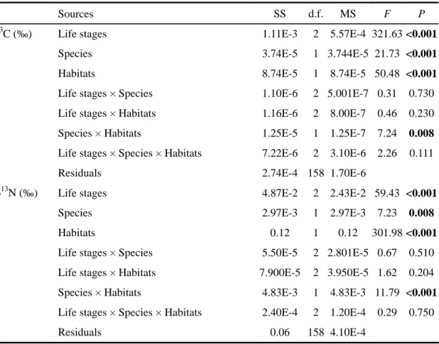
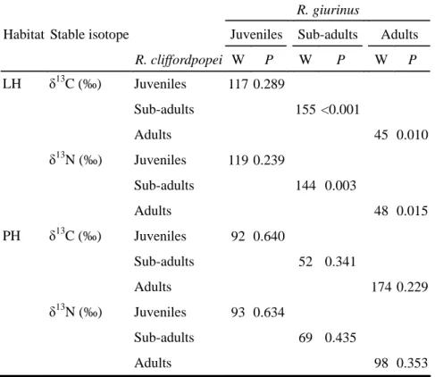
The stable isotopic values of food resources showed no significant differences between LH and PH (Mann-Whitney tests, P > 0.05). After examination of normality and variances homogeneity of data using Kolmogorov- Smirnov and Levene’s tests, three-way analyses of variance (ANOVA) were used to test the differences of stable isotopic values (δ13C and δ15N were the inverse transformed and tested separately) between life stages, species and habitats. If species showed significant effects on stable isotopic values, Mann-Whitney tests were used to test for differences between species within habitat for the same life stage.

The contributions of potential food resources to the diet of the two species were estimated using stable isotope mixing models (Stable Isotope Analysis in R; Parnell et al., 2008). Since there are no available trophic fractionation factor (TEF) values for the two goby species, we used an averaged TEF with a large SD as suggested by Inger et al. (2010). Here, the input TEF was 1.0 ± 1.0 ‰ (mean ± SD) for δ13C and 3.3 ± 1.0 ‰ (mean ± SD) for δ15N (Inger et al., 2010). Mean δ13C and δ15N values (±SD, n=3) of potential food resources in each habitat were used in the models. As life stages and habitats significantly affected the values of δ13C and δ15N, the models were run separately for different life stages in each habitat. Finally, the predicted percentage of contribution (mean ± SD) of each food source to the diet of the two species at the three life stages was averaged.

2.3.3 Age, growth, reproduction and population dynamics

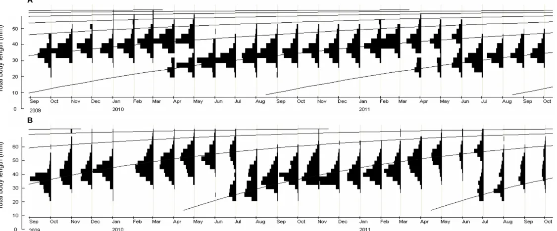
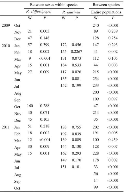
Age was determined by reading scales. Monthly body length-frequency was used to analyze cohort structures. In the same month, Kolmogorov-Smirnov (K-S) test was used to test differences in body length-frequency between males and females within species, and between species for the entire populations (including males, females and those unidentifiable for sexes).

(37)

LT and MT: log10 MT = a + b log10 LT. The mean LT and body condition were

compared between males and females within species, and between species for the entire populations using Mann-Whitney test and analyses of covariance (ANCOVAs) with LT as a covariate, respectively. Second, growth patterns were described by von Bertalanffy growth function (von Bertalanffy, 1938): Lt = L∞ [- e -K (t - t0)], where Lt is

the total body length at the time t, L∞ is the asymptotic length, K is the von

Bertalanffy growth coefficient, t0 is the theoretical age at LT = 0. VBGF was only

estimated for the entire populations because the sexes of most individuals were unidentifiable by macroscopic appearances of gonads in five months of a year. The function parameters were estimated using Electronic Length Frequency Analysis (ELEFAN) in the FiSAT II package (FAO – ICLARM Fish Stock Assessment Tools, Version 1.2.2, Gayanilo et al., 2005). t0 is was calculated as log10 (-t0) = -0.392 -

0.275 log10L∞ - 1.038 log10K (Pauly, 1979).

Reproduction cycles were estimated using gonado-somatic indices (IG) of

females, which were calculated for each mature specimen using the formula IG = 100

MG / MT. The onset and duration of reproduction seasons were quantified based on

the occurrence of individuals with stage-IV ovaries. The intensity of reproduction activities was determined by comparing IG and the proportions of different ovary

developmental stages between sampling dates. Logistic regression models were then used to quantify the proportion of mature males and females (stage IV and V,) at any LT using binomial maturity data (immature 0, mature 1). LT at which 50 % of

individuals are sexually mature was defined as the mean size of maturity (Lm50). A

log-likelihood ratio tests were used to test the differences of Lm50 between sexes

within each species. Mann-Whitney tests were used to test for potential differences in LT between males and females within each species.

Population dynamics of the two species were described using mortality and catch per unit effort (CPUE) of the fyke nets. Specifically, mortality calculations were conducted using the procedures in FiSAT II package (Gayanilo et al., 2005). Total mortality (Z, i.e. the sum of natural and fishing mortality) was estimated using

(38)

length-converted catch curves (Pauly, 1983). This method pools a long series of samples that represent a steady-state population and generate a single frequency distribution accounting for their relative importance. Z is then calculated on the descending part of this single global distribution (Pauly, 1983). Natural mortality (M) is correlated with asymptotic length (L∞), the von Bertalanffy growth coefficient (K),

and mean environmental temperature (T) by the Pauly’s M equation (Pauly, 1987): ln(M) = -0.015 - 0.279 ln(L∞) + 0.654 ln(K) + 0.463 ln(T). The mean annual

temperature used for M estimates was 18.7 °C. It was averaged from the monthly temperatures of Erhai Lake from October 2009 to October 2011. Fishing mortality (F) was then obtained by subtracting M from Z. The exploitation ratio (E) was calculated as E = F/Z.

Finally, catch per unit effort (CPUE, ind. net-1 day-1) of the fyke nets were calculated monthly and defined as the number of goby species caught in one net per day. Differences of CPUE (log-transformed) between species and months were tested using repeated-measures ANOVA (RM-ANOVA) with species as a fixed factor and months as a random factor. Sphericity assumption was tested using Mauchly’s test and the degrees of freedom were adjusted by Greenhouse–Geisser Epsilon when data violated the assumption of sphericity. In the same month, Mann-Whitney was subsequently used to test the differences in CPUE between species if species have significant effects on CPUE. The same approaches were used to test the differences in CPUE between sexes (fixed factors) within species and months (random factors).

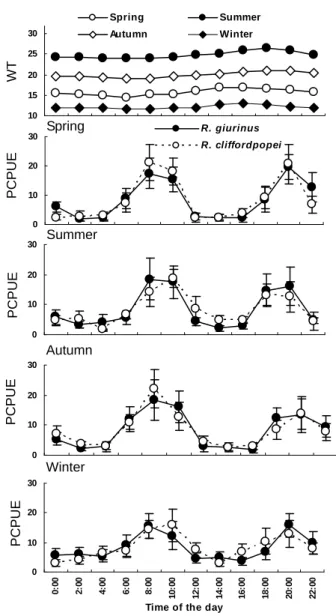
2.3.4 Activity level and feeding rhythm

The diel and seasonal activity were determined using the percentage of catch per unit effort (PCPUE, %) of benthic fyke nets, which was calculated as: 100 × number of individuals caught in a given two hours per net / total number of individuals caught in 24 hours of day per net. The differences in PCUPE (log (x+1) transformed) among

(39)

significant effects on CPUE, one-way ANOVAs were subsequently used to test the differences in PCPUE between seasons within species. Multiple comparisons among means were conducted using Tukey’s HSD post-hoc test when significant difference were identified by one-way ANOVAs.

The diel and seasonal feeding rhythm were determined using the percentage of empty gut (PEG) and weight of gut content (WGC). PEG was calculated as: FEG (%) = 100 number of empty guts/ number of total guts. WGC was calculated as: WGC (%) = 100 × food weight of non-empty gut / eviscerated weight of the body. Mann-Whitney test was used to test the differences in PEG among seasons within species, and between the two species within the same season. The differences in WGC (log (x+1) transformed) among seasons and species were tested using Mixed-Effects Models with seasons and species as fixed factors and time of the day as a random factor. The subsequent analyses were the same as used for PCPUE.

Normality and homogeneity of data were determined using one-sample Kolmogorov–Smirnov test and Levene’s test. All statistical analyses were performed using R version 2.14.2 (R Development Core Team 2012).