HAL Id: hal-03042946
https://hal.archives-ouvertes.fr/hal-03042946
Submitted on 18 Dec 2020
HAL is a multi-disciplinary open access
archive for the deposit and dissemination of
sci-entific research documents, whether they are
pub-lished or not. The documents may come from
teaching and research institutions in France or
abroad, or from public or private research centers.
L’archive ouverte pluridisciplinaire HAL, est
destinée au dépôt et à la diffusion de documents
scientifiques de niveau recherche, publiés ou non,
émanant des établissements d’enseignement et de
recherche français ou étrangers, des laboratoires
publics ou privés.
Large-scale features of Pliocene climate: results from the
Pliocene Model Intercomparison Project
A. Haywood, D. Hill, A. Dolan, B. Otto-Bliesner, F. Bragg, W.-L. Chan, M.
Chandler, C. Contoux, H. Dowsett, A. Jost, et al.
To cite this version:
A. Haywood, D. Hill, A. Dolan, B. Otto-Bliesner, F. Bragg, et al.. Large-scale features of Pliocene
climate: results from the Pliocene Model Intercomparison Project. Climate of the Past, European
Geosciences Union (EGU), 2013, 9 (1), pp.191-209. �10.5194/cp-9-191-2013�. �hal-03042946�
Clim. Past, 9, 191–209, 2013 www.clim-past.net/9/191/2013/ doi:10.5194/cp-9-191-2013
© Author(s) 2013. CC Attribution 3.0 License.
Climate
of the Past
Large-scale features of Pliocene climate: results from the Pliocene
Model Intercomparison Project
A. M. Haywood1, D. J. Hill1,2, A. M. Dolan1, B. L. Otto-Bliesner3, F. Bragg4, W.-L. Chan5, M. A. Chandler6, C. Contoux7,8, H. J. Dowsett9, A. Jost8, Y. Kamae10, G. Lohmann11, D. J. Lunt4, A. Abe-Ouchi5,12, S. J. Pickering1, G. Ramstein7, N. A. Rosenbloom3, U. Salzmann13, L. Sohl6, C. Stepanek11, H. Ueda10, Q. Yan14, and Z. Zhang14,15 1School of Earth and Environment, Earth and Environment Building, University of Leeds, Leeds, LS2 9JT, UK
2British Geological Survey, Keyworth, Nottingham, UK
3National Center for Atmospheric Research, Boulder, Colorado, USA
4School of Geographical Sciences, University of Bristol, University Road, Bristol, BS8 1SS, UK 5Atmosphere and Ocean Research Institute, University of Tokyo, Kashiwa, Japan
6Columbia University – NASA/GISS, New York, NY, USA
7Laboratoire des Sciences du Climat et de l’Environnement, Saclay, France
8Unit´e Mixte de Recherche 7619 SISYPHE, Universit´e Pierre-et-Marie Curie Paris VI, Paris, France 9US Geological Survey, MS 926A, 12201 Sunrise Valley Dive, Reston, VA 20192, USA
10Graduate School of Life and Environmental Sciences, University of Tsukuba, Tsukuba, Japan 11Alfred Wegener Institute for Polar and Marine Research, Bremerhaven, Germany
12Research Institute for Global Change, JAMSTEC, Yokohama, Japan
13Faculty of Engineering and Environment, Northumbria University, Newcastle upon Tyne, NE1 8ST, UK 14Institute of Atmospheric Physics, Chinese Academy of Sciences, Beijing, China
15Bjerknes Centre for Climate Research, Bergen, Norway
Correspondence to: A. M. Haywood ([email protected])
Received: 6 July 2012 – Published in Clim. Past Discuss.: 30 July 2012
Revised: 12 December 2012 – Accepted: 23 December 2012 – Published: 25 January 2013
Abstract. Climate and environments of the mid-Pliocene
warm period (3.264 to 3.025 Ma) have been extensively stud-ied. Whilst numerical models have shed light on the nature of climate at the time, uncertainties in their predictions have not been systematically examined. The Pliocene Model Inter-comparison Project quantifies uncertainties in model outputs through a coordinated multi-model and multi-model/data in-tercomparison. Whilst commonalities in model outputs for the Pliocene are clearly evident, we show substantial vari-ation in the sensitivity of models to the implementvari-ation of Pliocene boundary conditions. Models appear able to repro-duce many regional changes in temperature reconstructed from geological proxies. However, data/model comparison highlights that models potentially underestimate polar am-plification. To assert this conclusion with greater confidence, limitations in the time-averaged proxy data currently avail-able must be addressed. Furthermore, sensitivity tests
ex-ploring the known unknowns in modelling Pliocene climate specifically relevant to the high latitudes are essential (e.g. palaeogeography, gateways, orbital forcing and trace gasses). Estimates of longer-term sensitivity to CO2(also known as Earth System Sensitivity; ESS), support previous work sug-gesting that ESS is greater than Climate Sensitivity (CS), and suggest that the ratio of ESS to CS is between 1 and 2, with a “best” estimate of 1.5.
1 Introduction
1.1 The mid-Pliocene warm period
The mid-Pliocene warm period (mPWP) represents an in-terval of warm and stable climate between 3.264 and 3.025 Ma BP (Dowsett et al., 2010; Haywood et al., 2010).
It sits within the Piacenzian Stage of the Late Pliocene ac-cording to the geological timescale of Gradstein et al. (2004). The recent redefinition of the base of the Pleistocene to in-clude the Gelasian had led to this interval also being referred to as the mid-Piacenzian warm period (Dowsett et al., 2012), but we retain the use of mid-Pliocene warm period here for consistency with previous work.
Both geological data and climate model outputs have shed light on the nature of mid-Pliocene climate and environ-ments. During warm phases of the mid-Pliocene, highlighted by negative excursions in δ18O from benthic foraminifera, Antarctic and/or Greenland ice volume may have been re-duced (Lunt et al., 2008; Hill et al., 2010; Naish et al., 2009; Pollard and DeConto, 2009; Dolan et al., 2011), and between 2.7 and 3.2 Ma BP peak sea level is estimated to have been 22 ± 10 m higher than modern (Dowsett and Cronin, 1990; Miller et al., 2012). Sea surface temperatures (SSTs) were warmer (Dowsett et al., 2010), particularly in the higher lati-tudes and upwelling zones (e.g. Dekens et al., 2007; Dowsett et al., 2012). Sea ice cover also declined substantially (e.g. Cronin et al., 1993; Polyak et al., 2010; Moran et al., 2006). On land, the global extent of arid deserts decreased, and forests replaced tundra in the Northern Hemisphere (e.g. Salzmann et al., 2008). The global annual mean temperature may have increased by more than 3◦C (e.g. Haywood and Valdes, 2004). Meridional and zonal temperature gradients were reduced, which had a significant impact on the Hadley and Walker circulations (e.g. Contoux et al., 2012; Haywood et al., 2000; Kamae et al., 2011). The East Asian Summer Monsoon, as well as other monsoon systems, may have been enhanced (e.g. Wan et al., 2010).
Given the abundance of proxy data, the mPWP has become a focus for data/model comparisons that attempt to analyse the ability of climate models to reproduce a warm climate state in earth history (e.g. Haywood and Valdes, 2004; Salz-mann et al., 2008; Dowsett et al., 2011, 2012). Furthermore, the mPWP has been proposed as an important interval to as-sess the sensitivity of climate to near-current concentrations of carbon dioxide (CO2)in the long term (hundreds to thou-sands of years; Lunt et al., 2010).
1.2 Assessing uncertainty in models
Whilst a considerable number of climate simulations are available for the mPWP, they have been conducted using only a few climate models. Although there appears to be agree-ment among the models over certain aspects of climate dur-ing the mPWP (e.g. Haywood et al., 2000, 2009), there are likely to be significant differences in the details of their sim-ulations, particularly regionally (Haywood et al., 2009). In-consistencies are to be expected due to structural differences in models, and from differences in experimental design. The exploration of uncertainty in model simulations of past cli-mate has taken three primary forms. The first two include the use of a single model to either perform boundary condition sensitivity experiments (e.g. Haywood et al., 2007; Lunt et
al., 2008; Robinson et al., 2011), or to perform a perturbed physics ensemble (e.g Plio-QUMP; e.g. Pope et al., 2011). The third method uses a standardised experimental design in an ensemble composed of different climate models (a multi-model ensemble; e.g. Braconnot et al., 2007).
The Paleoclimate Modelling Intercomparison Project (PMIP) was initiated in 1991 to co-ordinate the systematic study of climate models, and to assess their ability to sim-ulate past climates (e.g. Joussaume and Taylor, 1995; Hoar et al., 2004; Zheng et al., 2008). PMIP also encourages the preparation of global reconstructions of palaeoclimates that can be used to evaluate climate models (e.g. Prentice and Webb, 1998). The focus of the studies carried out by PMIP has, until recently, been largely focussed on the Last Glacial Maximum and the mid-Holocene. However, in 2008 the Pliocene Modelling Intercomparison Project (PlioMIP) was added as a component of PMIP. Previously, there had only been limited efforts in documenting differences in model simulations of the mPWP. For example, Haywood et al. (2000) attempted a model intercomparison between ver-sions of the Hadley Centre for Climate Prediction and Re-search, the Goddard Institute for Space Studies (GISS) and National Center for Atmospheric Research (NCAR) climate models. This comparison was hampered by the fact that the experimental design used within these studies varied.
Haywood et al. (2009) compared the outputs from two mPWP experiments using versions of the Hadley Centre and Goddard Institute for Space Studies atmosphere-only climate models (HadAM3 and GCMAM3) in a more systematic way. Whilst the models were consistent in the simulation of large-scale differences in surface air temperature and total pre-cipitation rates, significant variations were noted at regional scales (i.e. in the Arctic). Terrestrial data/model comparison indicated that HadAM3 provided a closer fit to proxy data (biome distributions) in the mid- to high latitudes. However, GCMAM3 performed better than HadAM3 in the tropics.
Whilst the scope of the model intercomparison presented in Haywood et al. (2009) was limited, it served to encourage the palaeoclimate modelling community to establish a larger model intercomparison project (PlioMIP). Here we present an initial model intercomparison focussed on the large-scale features of mPWP climate derived from the PlioMIP ensem-ble. PlioMIP established the design for two initial exper-iments. Experiment 1 used atmosphere-only climate mod-els (AGCMs). Experiment 2 utilised coupled atmosphere– ocean climate models (AOGCMs) where SSTs and sea ice were predicted variables. We focus on the presentation of the global annual mean surface air temperature response in Experiment 1 and 2, zonal patterns of temperature and pre-cipitation change, polar amplification, comparisons of model results to proxy data, and finally calculations of longer-term climate sensitivity as defined by Lunt et al. (2010; Earth System Sensitivity).
A. M. Haywood et al.: Results from the Pliocene Model Intercomparison Project 193 2 Boundary conditions and experimental design
2.1 Participating modelling groups
Details of participating groups and models, and which ex-periment each group performed (Exex-periment 1 or 2 or both), can be found in Table 1. For Experiment 1 seven modelling groups completed and submitted data from their model in-tegrations. For Experiment 2 eight modelling groups com-pleted and submitted data. The models used in both Experi-ment 1 and 2 sample differing levels of complexity and res-olution from higher-resres-olution IPCC AR5-class models, to intermediate resolution models. Details of boundary condi-tions and their implementation in each model, as well as the basic climatologies from the majority of the models used in this study, can be found in a PlioMIP special edi-tion of the Journal Geoscientific Model Development (http: //www.geosci-model-dev.net/special issue5.html).
2.2 Boundary conditions
Full details of the boundary conditions used for PlioMIP Ex-periments 1 and 2 are provided in Haywood et al. (2010) and Haywood et al. (2011), respectively. In brief both exper-iments utilised the US Geological Survey PRISM3D bound-ary condition data set (Dowsett et al., 2010). For Experi-ment 1, this included information on monthly SSTs and sea ice distributions, vegetation cover, sea level, ice sheet extent and topography. For Experiment 2 modelling groups were given the choice of how to initialise their ocean model for the mPWP. They could spin up their model from a stan-dard pre-industrial control run, or specify the PRISM3D data set of ocean temperatures (Dowsett et al., 2009). Given the challenging nature of changing the land/sea mask in some atmosphere–ocean climate models, two versions of Pliocene boundary conditions were provided for both Exper-iment 1 and 2. The preferred data set included a change in the land/sea mask accommodating the removal of the West Antarctic Ice Sheet (WAIS), an increase in sea level of 25 m, and the infilling of the Hudson Bay. The alternate data set specified no changes in the land/sea mask but did remove the WAIS as far as possible by reducing topography down to sea level. The differences between the preferred and al-ternate boundary condition data sets are most striking over West Antarctica, which is fully deglaciated in the preferred data set, but set to near sea level and covered with tundra vegetation in the alternate boundary condition data set. The selection of preferred or alternate boundary conditions for each participating group is provided in Table 1. The impact on predictions of Pliocene climate from the selection of ei-ther preferred or alternate boundary condition protocols will be examined within single models set up with either bound-ary condition option in the near future.
NetCDF versions of all boundary conditions used for PlioMIP Experiment 1 and 2, along with guidance notes
for boundary condition implementation can be found at http://geology.er.usgs.gov/eespteam/prism/prism pliomip data.html. They have also been uploaded as a Supplement to Haywood et al. (2011).
2.3 Experimental design
The design of Experiment 1 and 2 is outlined in Haywood et al. (2010) and Haywood et al. (2011), respectively. In both experiments the atmospheric concentration of carbon diox-ide (CO2)was set at 405 ppmv. This value is towards the up-per limit of the uncertainty range provided by recently pub-lished CO2proxy records (e.g. Pagani et al., 2010; Seki et al., 2010; Bartoli et al., 2011). All other trace gasses were specified at a pre-industrial concentration and the selected orbital configuration was unchanged from modern. A 50 yr integration length was specified as a minimum for Experi-ment 1, with the final 30 yr used to calculate the required cli-matological means. A minimum integration length of 500 yr was specified for Experiment 2, which is long enough to al-low at least the surface climatology and oceans to interme-diate depth to reach an equilibrium condition. Again the fi-nal 30 yr were used to calculate climatological means. Re-quired fields and data formats that all groups were asked to provide can be found at http://geology.er.usgs.gov/eespteam/ prism/prism pliomeet11.html.
3 Results: PlioMIP Experiments 1 and 2
3.1 Global annual mean temperature change and hydrological response
For the Experiment 1 ensemble, a range of global annual mean SAT anomalies from 1.97 to 2.80◦C is simulated, while in Experiment 2, the ensemble range is between 1.84 and 3.60◦C (Table 2). No direct relationship between the magnitude of Pliocene SAT anomaly and Climate Sensitivity (the stated equilibrium temperature response to a doubling of CO2in the model) is seen (Table 2), demonstrating the im-portance of long-term climate drivers in mid-Pliocene warm-ing. However, we note that MIROC4m and the COSMOS models have the two highest mid-Pliocene global annual SAT anomalies, as well as the highest published Climate Sensitiv-ity estimates, implying CO2and fast feedbacks to be among the primary drivers. SAT anomalies over land (2.1 to 5.1◦C) are greater, and show a larger spread of response, than either SATs over the oceans or SSTs. This is to be expected given the additional complications of orography and vegetation and their influence on SAT over land. SATs over the oceans in-crease by 1.5 to 3.2◦C and SSTs increase by 1.1 to 2.2◦C (Fig. 1).
For Experiment 1 global annual mean precipitation rates increase by 0.04 to 0.11 mm day−1(Fig. 1). The changes in global precipitation in Experiment 1 are dominated by the increases over the land, whereas the specified increases in
T able 1. In Experiment 2 precipitation rates increase further to ∼ 0.09 to 0.18 mm day − 1 . Details of climate mode ls used with the PlioMIP Experiment 1 and 2 ensembles (a to g), plus details of boundary conditions (h and i), and published climate sensiti vity v alues (◦ C) for each Experiment 2 model (j). (c) (d) (e) (f) (g) (h) (i) (j) (a) (b) Atmosphere Ocean* Sea Ice* Coupling* Land Soils, Plants, PlioMIP Experiment 1 BC PlioMIP Experiment 2 BC Climate Model ID, Sponsor(s), T op Resolution Resolution Z Coord., Dynamics, Leads, Flux adjustments, Routing, (Hayw ood et al., 2010) (Hayw ood et al., 2011) Sensiti vity V intage Country References T op BC, References References References References Preferred/Alternate Preferred/Alternate (◦ C)* CCSM4, 2010 National Center for Atmospheric Research, USA T op = 2.2 hP a 0 .9 × 1 .25 ◦ , L26 Neale et al. (2013) 1 ◦ × 1 ◦ , L60 Depth, free surf ace Smith et al. (2010); Danabasoglu et al. (2012) Rheology , melt ponds Holland et al. (2012); Hunk e and Lipscomb (2010) No adjustments Gent et al. (2012) Layers, canop y, routing La wrence et al. (2012) Not Run Alternate Rosenbloom et al. (2012) 3.2 MIR OC4m, 2004 Center for Climate System Research (Uni. T ok yo, National Inst. for En v. Studies, Frontier Research Cen-ter for Global C hange, JAMSTEC), Japan T op = 30 km T42 (∼ 2 .8 ◦ × 2.8 ◦ ) L20 K-1 De v elopers (2004) 0.5 ◦ –1.4 ◦ × 1.4 ◦ , L43 Sigma/depth free surf ace K-1 De v elopers (2004) Rheology , leads K-1 De v elopers (2004) No adjustments K-1 De v elopers (2004) Layers, canop y, routing K-1 De v elop-ers (2004); Oki and Sud (1998) Preferred Chan et al. (2011) Preferred Chan et al. (2011) 4.05 HadAM3, 1997 Hadle y Centre for Climate Prediction and Research/Met Of fice UK T op = 5 hP a 2.5 ◦ × 3.75 ◦ , L19 Pope et al. (2000) Prescribed Prescribed Atmosphere-only Layers, canop y, routing Cox et al. (1999) Preferred Bragg et al. (2012) Not Run – HadCM3, 1997 Hadle y Centre for Climate Prediction and Research/Met Of fice UK T op = 5 hP a 2.5 ◦ × 3.75 ◦ , L19 Pope et al. (2000) 1.25 ◦ × 1.25 ◦ , L20 Depth, rigid lid Gordon et al. (2000) Free drift, leads Cattle and Crossle y (1995) No adjustments Gordon et al. (2000) Layers, canop y, routing Cox et al. (1999) Not Run Alternate Bragg et al. (2012) 3.1 GISS-E2-R, 2010 N ASA/GISS, USA T op = 0.1 hP a 2 ◦ × 2.5 ◦ , L40 Schmidt et al. (2013) 1 ◦ × 1.25 ◦ , L32 Mass/area, free surf ace Hansen et al. (2007) Rheology , leads Liu et al. (2003); Schmidt et al. (2013) Schmidt et al. (2013) Layers, canop y, routing Kiang et al. (2006) Not run Preferred Chandler et al. (2012) 2.7 to 2.9 COSMOS COSMOS-landv eg r 2413, 2009 Alfred W egener Institute, German y T op = 10 hP a T31 (3.75 ◦ × 3.75 ◦ ), L19 Roeckner et al. (2003) Bipolar orthogonal curvilinear GR30, L40 (formal 3.0 ◦ × 1.8 ◦ ) Depth, free surf ace Marsland et al. (2003) Rheology , leads Marsland et al. (2003), follo wing Hibler (1979) No adjustments Jungclaus et al. (2006) Layers, canop y, routing Raddatz et al. (2007), Hagemann and D ¨umenil (1998), Hage-mann and Gates (2003) Preferred Stepanek and Lohmann (2012) Preferred Stepanek and Lohmann (2012) 4.1 LMDZ5, 2010 Laboratoire des Sciences du Climat et de l’En vironnement (LSCE), France T op = 70 km 3.75 ◦ × 1.9 ◦ , L39 Hourdin et al. (2006, 2012) Prescribed Prescribed Atmosphere-only Layers, canop y, routing Krinner et al. (2005) Alternate and Preferred Contoux et al. (2012) Not Run – IPSLCM5A, 2010 Laboratoire des Sciences du Climat et de l’En vironnement (LSCE), France T op = 70 km 3.75 ◦ × 1.9 ◦ , L39 Hourdin et al. (2006, 2012) 0.5 ◦ –2 ◦ × 2 ◦ , L31 Free surf ace, Z-coordinates Dufresne et al. (2 012), Madec et al. (1997) Thermodynamics, Rheology , Leads Fichefet and Morales-Maqueda (1997, 1999), No adjustment Marti et al. (2010), Dufresn e et al. (2012) Layers, canop y, rout-ing, phenology Krinner et al. (2005), Marti et al. (2010), Dufresne et al. (2012) Not Run Alternate Contoux et al. (2012) 3.4 MRI-CGCM 2.3, 2006 Meteorological Research Institute and Uni v ersity of Tsu kuba, Japan T op = 0.4 hP a T42 (∼ 2 .8 ◦ × 2.8 ◦ ) L30 Y ukimoto et al. (2006) 0.5 ◦ –2.0 ◦ × 2.5 ◦ , L23 Depth, rigid lid Y ukimoto et al. (2006) Free drift, leads Mellor and Kantha (1989) Heat, fresh w ater and mo mentum (12 ◦ S– 12 ◦ N) Y ukimoto et al. (2006) Layers, canop y, routing Sellers et al. (1986); Sato et al. (1989) Alternate Kamae and Ueda (2012) Alternate Kamae and Ueda (2012) 3.2 NorESM-L (CAM4), 2011 Bjerknes Centre for Climate Research, Ber gen, Norw ay T op = 3.5 hP a T31 (∼ 3 .75 ◦ × 3.75 ◦ ), L26 (CAM4) G37 (∼ 3 ◦ × 3 ◦ ), L30 isop ycnal layers Same as CCSM4 Same as CCSM4 Same as CCSM4 Alternate Zhang and Y an (2012) Alternate Zhang et al. (2012) 3.1 CAM3.1, 2004 Institute of Atmospheric Ph ysics, Chinese Academy of Sciences, Beijing, China T42 (2.8 ◦ × 2.8 ◦ ), L26 Collins et al. (2004) Prescribed Prescribed Atmosphere-only Layers, canop y, routing Bonan et al. (2002) Alternate Y an et al. (2012) Not Run – ∗ Rele v ant for climate models used for Experime nt 2 only .
A. M. Haywood et al.: Results from the Pliocene Model Intercomparison Project 195
Fig. 1. (a) Global annual mean surface air temperature anomalies (mPWP minus pre-industrial control experiment) from each model in the PlioMIP Experiment 1 and 2 ensembles. Published estimates of Experiment 2 models’ equilibrium climate sensitivity also provided, alongside the global mean SST anomalies for each model in Experiment 2. Annual mean surface air temperature anomalies from each Experiment 1 (b) and Experiment 2 (c) simulation separated into response over land and oceans. (d) SAT warming over land against ocean SAT warming for all Experiment 2 simulations. Global, land and ocean annual mean total precipitation rate anomalies for all simulations from Experiment 1 (e) and Experiment 2 (f).
SSTs are associated with very little increase in precipitation over the ocean. In Experiment 2 precipitation rates increase further to ∼ 0.09 to 0.18 mm day−1. MIROC4m, COSMOS and HadCM3 simulate the largest changes in total precipi-tation rate in the ensemble. A much smaller contrast is seen between increases on the land and over the ocean, although the partitioning of this increase is highly variable from model to model (Fig. 1).
3.2 Multi-model mean surface air temperature and precipitation (Experiment 1)
To facilitate the production of annual multi-model mean (MMM) SAT and precipitation rate anomalies (Experiment 1 and 2), as well as SST anomalies (for Experiment 2 only), each participating models’ mPWP simulation was differ-enced to its respective pre-industrial control experiment.
Table 2. (a) Experiment 2 models included in the assessment of Cli-mate Sensitivity (CS) versus Earth System Sensitivity (ESS) plus the ensemble means; (b) calculated anomaly in global annual mean surface air temperatures (◦C); (c) published estimates of CS (◦C); (d) calculated estimates of ESS (◦C); (e) ratio of ESS to CS; (f) en-ergy balance at the Top of the Atmosphere in W m−2for the control and Pliocene experiments.
(a) (d) (f)
Experiment 2 (b) (c) ESS (◦C) TOA Energy
Climate Pliocene CS = mPWP (e) Balance (W m−2) Models/Mean 1T(◦C) (◦C) 1T ·1.88 ESS/CS CTRL:Pliocene CCSM4 1.86 3.2 3.51 1.1 −0.1 : 0.1 COSMOS 3.60 4.1 6.77 1.7 2.4 : 2.3 GISS-E2-R 2.12 2.7 3.98 1.5 0.45 : 0.15 HADCM3 3.27 3.1 6.16 2.0 −0.79 : 0.16 IPSLCM5A 2.18 3.4 4.10 1.2 0.21 : 0.81 MIROC4m 3.46 4.05 6.51 1.6 0.81 : 0.90 MRI-CGCM 2.3 1.84 3.2 3.45 1.1 2.9 : 3.0 NorESM-L 3.27 3.1 6.14 2.0 2.1 : 2.1 Ensemble Mean 2.66 3.36 5.01 1.5 –
These data were then re-gridded on to the regular 2◦×2◦ lat-itude/longitude grid of the PRISM3D boundary conditions. MMM fields were then calculated as a simple mean of each of the individual model experiments. This allows us to evalu-ate the ensemble as a whole, without down-weighting any of the individual models. Future work may include evaluation of each individual model against mPWP data and the pro-duction of weighted MMM to make a combined model and data estimate of mPWP climate. Individual model anomalies for SAT and total precipitation rate on their common/local grids are included in Figs. S1 and S2 in the Supplement.
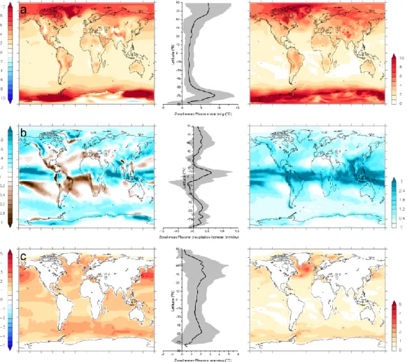
The MMM SAT anomaly (Fig. 2) from pre-industrial shows minimal change between 15◦north and south of the
Equator, with the exception of the eastern equatorial Pacific, which displays a warming of up to 3◦C. Between 15◦ and 90◦ north and south of the Equator the SAT anomaly be-comes progressively stronger, particularly over Greenland and the Arctic Basin, and in areas of West and East Antarc-tica. The zonal MMM SAT anomaly shows little or no change in the tropics and a clear polar amplification of temperatures. Temperatures increase by > 10◦C in the Arctic and up to 20◦C in the Antarctic (Fig. 2).
Uncertainties within the MMM reconstruction can be eval-uated in terms of the spread of the predictions within the ensemble, with two standard deviations (2σ ) being a stan-dard measure (Le Treut et al., 2007). However, this ensem-ble is only small, so our use of this measure does not imply it is normally distributed, nor is it necessarily a 95 % confi-dence interval. Over the open oceans the models’ SATs do not vary significantly from one another due to SSTs being prescribed. A 2 σ of 1 to 4◦C is common in the MMM over land (Fig. 2). In regions dominated by ice sheets or sea ice, the 2 σ increases to 6 to 8◦C. In the same regions where the land/sea mask was altered (i.e. West Antarctica, the mar-gins of East Antarctica and the Hudson Bay), the 2 σ exceeds
8◦C; such high inter-model differences are attributable to the
application of either the PlioMIP preferred or alternate exper-imental design (Haywood et al., 2010, 2011).
For total precipitation rate, the MMM indicates a com-plex response in the tropics (Fig. 2). In the central and west-ern Pacific precipitation rates near the Equator are reduced by ∼ 1 mm day−1. At 15◦ north and south of the Equator, and in the eastern equatorial Pacific, precipitation rates in-crease by more than 2 mm day−1. Over the African conti-nent and the Indian sub-conticonti-nent precipitation rates gener-ally increase (0.1 to ∼ 2 mm day−1). Over the majority of the Indian Ocean precipitation rates are reduced. Over North America precipitation rates increase in the northwest and are reduced in the southwest. Over ice-free regions of Greenland and Antarctica precipitation rates increase. Finally, large in-creases in precipitation rate (> 2 mm day−1) are predicted in the northern North Atlantic and the Nordic Seas.
Such regional differences are reproduced in the zonal MMM mean precipitation anomaly (Fig. 2). Around the Equator precipitation rates decrease by ∼ 0.4 mm day−1. 15◦ north and south of the Equator precipitation rates increase by up to 0.3 mm day−1. The zonal MMM indicates increased precipitation rates in the Southern Hemisphere westerlies. In general precipitation rates increase in the Northern Hemi-sphere north of 30◦N and peak changes are seen at ∼ 80◦N. In the tropics the 2 σ within the Experiment 1 ensemble can exceed 3 mm day−1, whereas in most other areas the 2 σ is no greater than 1.5 mm day−1(Fig. 2).
3.3 Multi-model mean surface air/sea surface temperature/precipitation (Experiment 2)
The process for constructing annual MMMs for Experi-ment 2 was the same as that adopted for ExperiExperi-ment 1, except for the inclusion of SSTs. Individual model anomalies for SAT, total precipitation rate and SSTs on their common/local grids are included in Figs. S3, S4 and S5 in the Supplement. The LSCE and GISS modelling groups have recently pro-vided additional simulations for Experiment 2 to those used for the calculation of the MMMs. The degree to which these additional data alter the calculated MMM for Experiment 2 is shown in Fig. S7 in the Supplement. In the tropics the MMM indicates a general pattern of SAT warming of 1 to 2◦C over the oceans (Fig. 3). In the same region warming over the land ranges from 1 to 6◦C. From the mid to high latitudes a pattern of progressively larger SAT anomalies is predicted reaching a maximum change over Greenland and the Arc-tic, West Antarctica and areas of East Antarctica. The zonal mean SAT anomaly displays ∼ 2◦C warming in the tropics, increasing to ∼ 6◦C and 9◦C in the high latitudes of the Northern and Southern Hemispheres, respectively (Fig. 3). The 2 σ around the zonal MMM SAT anomaly is broad in the high latitudes of both hemispheres. Models largely agree in their predictions of tropical SAT change over the oceans and land (with greater variation), whilst in the North Atlantic
A. M. Haywood et al.: Results from the Pliocene Model Intercomparison Project 197
Fig. 2. Multi-model means, zonal means and model 2σ from the Experiment 1 ensemble. (a) Mean annual surface air temperature anomaly (Experiment 1 Pliocene minus pre-industrial control) and (b) mean annual total precipitation rate anomaly (Experiment 1 Pliocene minus pre-industrial control). Shading around the zonal mean is the model 2 σ .
and the higher latitudes in general the 2 σ ranges from 2 to 10◦C (Fig. 3).
The MMM indicates a large increase in total precipita-tion rates between the Equator and 15◦N, which can ex-ceed 1 mm day−1(Fig. 3). In the Atlantic and Pacific Ocean basins, a reduction in precipitation rate is seen between the Equator and 15◦S–30◦S (0.1 to 1 mm day−1). Regions in-fluenced by the Indian and West African monsoons show a pattern of increased precipitation rates, and this is also seen in regions dominated by the mid-latitude storm tracks. The pattern of precipitation anomalies between the sub-tropics and mid-latitudes in the Northern Hemisphere (decline in the sub tropics and increases in the mid latitudes) is suggestive of a northward shift of the zone influenced by mid-latitude storms. Increased precipitation rates are predicted in ice-free regions of Greenland, West and East Antarctica. In the zonal MMM the pattern of enhanced precipitation rates from the Equator to 15◦N is replicated, as is the general trend for pre-cipitation rates to decrease from 15 to 30◦south. Precipita-tion rates in the mid-latitudes and to approximately 75◦north and south of the Equator are also enhanced by a maximum of 0.3 mm day−1. The 2 σ of model results which contribute to the MMM is large (0.1 to > 3 mm day−1) in the tropics with greater consistency between models in the extra tropics (Fig. 3).
The MMM SST anomaly shows a pattern of increased global SSTs (1 to 5◦C). Warmer mPWP SSTs are most
pro-nounced in the North Pacific, Southern Ocean and in parts of the North Atlantic. The zonal MMM for SSTs, along with
the calculated 2 σ , confirms these basic trends, whilst high-lighting regions of greater or lesser consistency between the model results. In the North Pacific the SST anomaly is large (up to 5◦C) and the standard deviation is generally no greater than 2◦C (Fig. 3). In contrast the SST response in the North Atlantic is weaker (2 to 3◦C), and at the same time the 2 σ from the ensemble is large (locally exceeding 4◦C). One model in the ensemble produces a different sign of change in this region in response to the implementation of Pliocene boundary conditions compared with other models (GISS-E2-R; see Fig. S5c in the Supplement). The reasons for this are discussed in Chandler et al. (2012) and the associated inter-active discussion of that paper. An additional Experiment 2 simulation from the GISS modelling group, utilising a differ-ent version of the GISS model with an improved represdiffer-enta- representa-tion of ocean mixing, provides a SST anomaly in the North Atlantic in broad agreement with the general response seen from all of the other models used within the Experiment 2 ensemble. The degree to which this additional simulation dif-fers from the original GISS simulation and how it alters the calculated MMM for SST in the North Atlantic is shown in Figs. S6 and S7 in the Supplement.
3.4 Multi-model means (Experiment 2 minus Experiment 1)
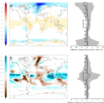
For annual MMM SAT anomalies, differences between Ex-periments 1 and 2 exceeding 1 or 2◦C are largely restricted to the North Atlantic and the Arctic (Fig. 4). The Nordic Seas and the Arctic east of Greenland exhibit differences
Fig. 3. Multi-model means, zonal means and model 2 σ from the Experiment 2 ensemble. (a) mean annual surface air temperature anomaly (Experiment 2 Pliocene minus industrial control), (b) mean annual total precipitation rate anomaly (Experiment 2 Pliocene minus pre-industrial control) and (c) mean annual sea surface temperature anomaly (Experiment 2 Pliocene minus pre-pre-industrial control). Shading around the zonal mean is the model 2 σ .
exceeding 6 to 8◦C due to a weaker SAT anomaly predicted in Experiment 2. In the Antarctic sea ice region the Exper-iment 2 MMM anomaly is also smaller than ExperExper-iment 1 (∼ 1 to 3◦C). In the tropics Experiment 2 generally displays a larger mean annual SAT anomaly than Experiment 1 by ∼ 1 to 2◦C. These trends are also reflected in the zonal MMM SAT difference between Experiment 2 and 1 anomaly. From the calculated differences in model 2 σ it is clear that the con-sistency of the MMM in high latitudes is substantially less in Experiment 2 than Experiment 1. This result is also repeated in the Southern Hemisphere sea ice region. In the tropics the calculated 2 σ on the MMM anomaly is far smaller than at the high latitudes (∼ 4◦ rather than 20◦C), highlighting a greater consistency seen in the results from Experiment 1 and 2 (Fig. 4).
Differences between the MMM and zonal MMM’s for Ex-periment 2 and 1 for total precipitation rate anomalies are particularly striking in the tropics (Fig. 4). In this region Ex-periment 2 predicts a larger anomaly in precipitation rates (wetter) over the oceans than Experiment 1. Conversely, the
Experiment 1 anomaly is greater in the tropics over land (drier) than Experiment 2 (Fig. 4). The calculated 2 σ on the Experiment 2 and 1 MMM total precipitation rate anoma-lies shows, as expected, an inverse pattern to that displayed for SAT. Model-predicted anomalies appear largely consis-tent to within 2 mm day−1in high and mid-latitudes, but are less consistent in the tropics (Fig. 4).
3.5 Temperature and precipitation anomalies in response to mPWP boundary conditions
For Experiment 1, and to a lesser degree Experiment 2, the MMM differences in mPWP climate are closely linked to the specified boundary conditions provided by the PRISM3D data set. Altered SST patterns, sea and land ice volumes are a first order control on the simulated variations of the mPWP climate relative to the pre-industrial. The variations in cli-mate are driven by changes in sensible and latent heat fluxes (SST-driven), and variations in ocean/atmosphere heat ex-change caused by differences in sea ice.
A. M. Haywood et al.: Results from the Pliocene Model Intercomparison Project 199
Fig. 4. Difference in multi-model mean anomalies between Experi-ment 2 and 1. (a) difference in mean annual SAT and zonal mean an-nual SAT anomalies. (b) difference in mean anan-nual and zonal mean annual total precipitation rate anomalies. Shading around the mean represents the model 2 σ .
3.5.1 Experiment 1
For Experiment 1 the MMM response in annual mean SAT and total precipitation rates are strongly controlled by the im-posed boundary conditions from the PRISM3D data set. At high latitudes, reductions in specified land and sea ice gen-erate a significant polar amplification of the SAT anomaly (Fig. 2), driven by local altitude changes and also ice/albedo feedbacks. This is augmented on land by a change in vege-tation distribution from tundra to forest type biomes, chang-ing surface albedo and evapo-transpiration rates. In the mid-latitudes, SAT anomalies are strongly controlled by local vegetation changes and also by elevated SSTs (Fig. 2). Increasing total precipitation rates outside the tropics are cor-related with SSTs, land and sea ice changes, and where veg-etation patterns differ most from modern. The response of precipitation in the tropics appears to be driven by reduced meridional SST gradients generally, as well as reduced zonal SST gradients in the tropical Pacific and Atlantic Oceans (Fig. 2). SST gradient changes have a significant effect on the strength of Hadley and Walker circulations, and poten-tially also generate a general broadening of the Hadley Cell, explaining the redistribution of precipitation (Kamae et al., 2011). Over North America the precipitation rate anomaly displays a dipole pattern (wetter in the northwest and drier in the southeast of the continent). This appears to be an atmo-spheric teleconnection to the reduced zonal SST gradient in the tropical Pacific (Fig. 2; warmer eastern equatorial Pacific
SSTs). These conclusions based on the MMM are consistent with published analyses of the individual model results (e.g. Chan et al., 2011; Contoux et al., 2012; Kamae and Ueda, 2012; Zhang and Yan, 2012; Koenig et al., 2012).
3.5.2 Experiment 2 minus Experiment 1
Experiment 2 displays a number of the general trends and drivers for predicted climate differences described already for Experiment 1, with a number of important exceptions. The primary difference between the MMMs for Experi-ment 1 and 2 is dominated by ExperiExperi-ment 2 displaying a weaker high latitude SAT anomaly and warmer tropical peratures (Fig. 4). This generates a steeper meridional tem-perature gradient. Zonal SAT gradients are also larger in Ex-periment 2 compared to ExEx-periment 1 in the tropical Pa-cific (Fig. 4). These combined differences impact on the sim-ulated precipitation rate response in the tropics in Experi-ment 2 through influencing the vigour of the Hadley and Walker circulations.
4 Surface air/sea surface temperature comparisons 4.1 Point-based comparison of SATs and SSTs
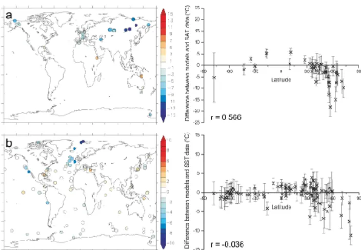
Figure 5 shows a traditional comparison of point-based proxy temperature anomalies to the MMM anomalies derived from Experiment 2. This analysis assesses the degree of agree-ment between the temperature anomalies of proxies and models, rather than comparing absolute temperature esti-mates. On land terrestrial temperature estimates are derived from Salzmann et al. (2008, 2013). In the Southern Hemi-sphere and tropics MMM SAT anomalies are within 3◦C of proxy anomalies. In the Northern Hemisphere, particu-larly beyond 40◦N, the MMM underestimates the magni-tude of SAT warming by as much as 15◦C. For the oceans SST anomalies are derived from Dowsett et al. (2010) and Dowsett et al. (2012). The analysis shown in Fig. 5 demon-strates a broad concordance between data and models apart from in the northern North Atlantic and Nordic Seas. Here the MMM underestimates the magnitude of change by as much as 8 to 10◦C. Whilst the difference between MMM SAT/SST and proxy-based SST anomalies is substantial in specific regions it is worth noting that 2 σ around the MMM can also be substantial reflecting the degree of model varia-tion within the PlioMIP ensemble.
4.2 Regional-scale comparison of SSTs and SATs
Due to the different spatial scales considered by proxy-data and model outputs it is not surprising to see the kind of dis-cord between proxies and model results seen in Fig. 5. To test the validity of the comparison previously shown, proxy and model simulations at a regional scale are analysed (Fig. 6). The globe is subdivided into the seven continents in the
Fig. 5. Point-based data/model comparison of (a) surface air tem-perature and (b) sea surface temtem-perature anomalies (modelled warming minus proxy data Pliocene warming) for Experiment 2. Error bars on the scatter plots refer to the 2 σ range derived from the Experiment 2 ensemble, while r is the Pearson correlation co-efficient between the modelled Pliocene warming anomaly and the data derived warming estimates.
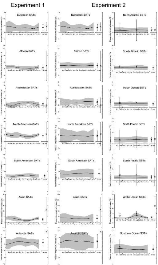
terrestrial realm and the seven major ocean basins in the ma-rine regime. Proxy temperature anomalies pertaining to each marine or terrestrial region were collated and averaged. For marine regions faunal analysis SST calculation methods pro-vide information on cold and warm month SSTs (Dowsett et al., 2010, 2012). Available Mg/Ca and alkenone palaeother-mometry based estimates available for a sub-section of ma-rine sites provide additional information on mean annual SSTs (Dowsett et al., 2010, 2012). These estimates are com-pared to regional mean annual and monthly changes in tem-perature computed from the Experiment 2 (marine and ter-restrial regions) and Experiment 1 (terter-restrial regions only) multi-model means. The calculated 2 σ values for SAT and SST derived from all the ensemble members are also in-cluded (Fig. 6).
In this analysis the general agreement between model outputs and SST proxy estimates for the Southern Ocean, North and South Pacific, Indian and South Atlantic Oceans highlighted in Fig. 5 is reiterated. In the Arctic Ocean, the model/data discord persists but is only marked when the model results are compared to geochemically based proxy mean annual SST estimates, rather than faunal analysis-based estimates for cold and warm month means. Any data/model discord in this region should be viewed with caution until multi-proxy temperature estimates are available from more marine localities in the Arctic.
For the North Atlantic, the regional comparison indicates more concordance between the models and proxy data than in the point-based analysis shown in Fig. 5, where the North Atlantic was shown as a clear region of major data/model discord. We interpret this difference as an indication of the models’ ability to simulate the average amount of warming
in the North Atlantic as a whole, whilst not necessarily repro-ducing the exact distribution of the SST increases vis-a-vis the PRISM3D localities used for SST reconstruction. Given the complex oceanography and steep SST gradients that exist in the North Atlantic (e.g. Kelly et al., 2010) this outcome is not surprising given the resolution of the ocean models used in this study.
In terms of data/model concordance over land there is agreement in most regions except for Asia where the Experi-ment 2 and 1 MMMs both underestimate the degree of MAT increase compared to the proxy data. Differences over Aus-tralia are at the limits of detection, while the single point over Antarctica is not representative of continental scale warm-ing and suffers from uncertain chronology (Hill et al., 2007). Over Asia the analyses shown in Figs. 5 and 6 highlight the greater degree of warming reconstructed in the continental interior and high latitudes in the proxies compared to the MMMs. The results presented in this section have demon-strated interesting regional features of data/model concor-dance/discordance. However, they should be viewed as a pre-liminary analysis. More detailed data/model comparison for the PlioMIP Experiment 2 ensemble will be subject of addi-tional studies in the near future.
5 Calculation of Earth System Sensitivity 5.1 What is Earth System Sensitivity?
Climate sensitivity (the temperature response of the earth to elevated CO2concentrations) is a concept which has received much attention, as it is a simple and easily understood metric which gives a first-order indication of the magnitude of pos-sible future climate change given increased CO2emissions (e.g. Charney, 1979; Hansen et al., 2008; Meinshausen et al., 2009).
Estimates of climate sensitivity, which are based on mod-els, are normally defined as the modelled global mean near surface air temperature equilibrium response to a sustained doubling of atmospheric CO2 concentration. In general, model-based estimates of climate sensitivity are most rele-vant for short timescales (< 100 yr), as typical climate mod-els do not include feedbacks which act on longer timescales, and/or are not often run out to full equilibrium (Lunt et al., 2010; Hansen et al., 2008). Furthermore, no model includes all possible feedbacks even on short timescales. For example, feedbacks associated with atmospheric chemistry, non-CO2 greenhouse gases, and aerosols are only just being included in state-of-the-art models.
Earth System Sensitivity (ESS) has been defined by Lunt et al. (2010) as the equilibrium global mean near-surface (∼ 2 m) air temperature response to a sustained doubling of atmospheric CO2concentrations, including all feedbacks and processes apart from those associated with the carbon cycle itself. By taking account of long timescale feedbacks, models
A. M. Haywood et al.: Results from the Pliocene Model Intercomparison Project 201
Fig. 6. Regional marine and terrestrial annual and monthly mean data/model comparisons. Comparison includes the calculated model 2 σ derived from Experiment 1 and 2 models regional averages. Left column: Experiment 1 terrestrial regions. Middle column: Experiment 2 terrestrial regions. Right column: Experiment 2 marine realm. Error bars on the data (crosses) are derived from spatial variability over the region (i.e. does not represent variability or uncertainty). In the annual means the stars represent the modelled annual mean and the crosses the proxy data. Terrestrial data comes from palynological and biome estimates (Salzmann et al., 2013). February and August SST estimates are derived from assemblage data, while annual mean SST data are Mg/Ca and alkenones estimates (Dowsett et al., 2010, 2012).
can be used to estimate ESS. Palaeo data are very useful tools in determining ESS, as they provide the potential for provid-ing the model with information on the long-term feedbacks, which are often problematic to model explicitly.
5.2 Previous estimates of ESS using the mPWP
The mPWP is useful for investigating the concept of ESS because it represents a world in quasi-equilibrium with high CO2for a sufficient period that long-term feedbacks are close to equilibrium. Using a combined model-data approach, Lunt et al. (2010) estimated ESS to be between 30 % and 50 % greater than CS. They took a climate model (HadCM3), and imposed changes to the CO2, orography, ice sheet and veg-etation model boundary conditions, which were consistent with changes observed in the mPWP palaeo record. They then evaluated the model simulation relative to mPWP SST records. Finally, they used a series of sensitivity studies to eliminate the orographic forcing effect, arguing that the re-maining temperature signal was an approximation to ESS.
5.3 Using PlioMIP Experiment 2 to inform estimates of ESS
Here, we use the PlioMIP simulations from Experiment 2 to estimate ESS, using a similar approach to Lunt et al. (2010). Since the PRISM3D orography in the PlioMIP experimental design is similar to modern (Sohl et al., 2009), our approach is actually significantly simpler than Lunt et al. (2010) be-cause we argue that in this case, the orographic effect is neg-ligible. In the PRISM2 data set, which was used to provide the boundary conditions for the Lunt et al. (2010) estimates, mPWP and modern orographies were less similar. As such, we consider the elevated CO2to be the ultimate forcing of the simulated mPWP warmth, and thus our simulations represent the equilibrium state of a world at 405 ppmv of CO2. To con-vert this to the usual definition of ESS (i.e. a CO2doubling from 280 to 560 ppmv), the Pliocene warming is multiplied by ln(560.0 / 280.0)/ln(405.0 / 280.0) = 1.88.
The global mean values are given in Table 2 for each model and the ensemble mean, along with the CS value from each model, and the ratio ESS/CS. There is a large spread in the ratio ESS/CS from 1.1 (CCSM4 and MRI-CGCM 2.3) to 2.0 (HadCM3 and NorESM-L). The ratio for the ensemble mean is 1.5. Therefore, the PlioMIP simulations give us con-fidence that ESS > CS, suggest ESS/CS is between 1.1 and 2, and imply a “best” estimate of 1.5.
A recent study (Palaeosens project members, 2012) has suggested a naming convention for distinguishing between estimates of climate and Earth system sensitivity, which highlights whether various processes are considered as forc-ings or feedbacks. In the notation of that study (which also recommends citing values in units of K/W m−2), we find here a palaeo sensitivity, Sp=S[CO2]=1.35 K/W m
−2(assuming a radiative forcing from a doubling of CO2 of 3.7 W m−2).
The subscript [CO2] of S[CO2] indicates that this estimate
of sensitivity includes possible carbon cycle feedbacks as a forcing. Also in the notation of that paper, the fast-feedback climate sensitivity, Sa=0.91 K/W m−2.
A first caveat to these calculations of ESS versus CS is that specific models used within the PlioMIP Experiment 2 ensemble have non-negligible top of the atmosphere energy imbalances (TOA). The rate at which models progress to-wards energy balance varies from model to model, and the specified integration length, whilst being the best that could be pragmatically hoped for, was insufficient to bring all the models into approximate energy balance (Table 2 column f). However, the difference in TOA energy balance between each models pre-industrial control and Pliocene simulations is always < 1 W m−2. If the models that display a larger than
∼0.5 W m−2imbalance are removed from the calculation of the ensemble mean ESS/CS, the ensemble mean ESS/CS still remains constant at 1.5. A further limitation is that there may be inconsistencies between the estimates of CS and ESS due to the fact that the CS estimates were not formally requested as part of PlioMIP. For example, integration length and initial condition may differ between the ESS and CS simulations.
A final caveat to our calculations of ESS is that changes in the Earth’s orbit are not relevant to calculations of either CS or ESS. If reconstructed changes in global ice volume or veg-etation distribution (i.e. the imposed longer term feedbacks) are even partly a function of orbital variability rather than CO2, the utility of the current experiments for understand-ing the sensitivity of climate in the context of future climate change is diminished. Initial transient mid-Pliocene climate simulations using Earth System Model of Intermediate Com-plexity are becoming available. Here CO2forcing and orbital forcing have been imposed in isolation and in concert, and have suggested that a significant percentage of the additional feedback to global temperature derived from changes in veg-etation cover and ice sheet extent may be attributable to or-bital forcing (Ganopolski et al., 2011).
6 Discussion and future outlook
6.1 PlioMIP Phase 2: recognising and reducing uncertainties (the PMIP Triangle)
The data/model comparisons shown in section 4 do not consider temporal variability and uncertainty of the proxy-estimated SST anomalies (see Dowsett et al., 2012). There-fore, whilst the identified patterns of data/model mismatch may appear convincing, they are likely to be an overestimate of the true level of discord between models and proxy data.
In any palaeo data/model comparison the cause of data/model mismatches will be complex and not attributable to a single factor in either the models or proxy data. In the context of PMIP three high-level causes of data/model discord require consideration. The first is limitations in
A. M. Haywood et al.: Results from the Pliocene Model Intercomparison Project 203
model physics and structure, the second is uncertainties in the interpretation of proxy records, and the third is limita-tions of experimental design within the models. This triangle of uncertainty, which we term the PMIP Triangle, serves as a useful guide to establish a well-balanced assessment of the causes of disagreement between proxy data and model out-puts.
In terms of the climate modelling for the Pliocene, PlioMIP is an effective means to quantify uncertainties in model predictions (the modelling vertex of the PMIP
Trian-gle). So far PlioMIP has identified an envelope of climate
possible from a collection of atmosphere-only and coupled atmosphere–ocean climate models set up to produce a single realisation of climate for the mPWP.
Given the known unknowns in providing models with “cor-rect” boundary conditions for the mPWP, it would be ad-vantageous for PlioMIP Phase 2 to focus on identifying a number of key sensitivity experiments to examine how poor constraints on atmospheric trace gasses, ice sheet configu-rations, palaeogeography and bathymetry could reduce the magnitude of data/model discord seen in the high latitudes of the Northern Hemisphere. Outlining a series of potential sen-sitivity tests, and allowing modelling groups to select which experiment or experiments they wish to run, would facilitate an efficient exploration of boundary condition uncertainty (experimental design vertex of the PMIP Triangle).
The final point of the PMIP Triangle to be considered is uncertainties in the interpretation of proxies which provide SAT and SST estimates. One of the most important of these uncertainties surrounds chronology and the time-averaged nature of the PRISM3D data set. Limitations in correlating one marine or land site to another over large geographical distances, favoured the establishment of a time slab in the Pliocene to which the ages of marine or terrestrial sites could be more confidently attributed (Dowsett and Poore, 1991). It also increased the potential amount of geological data that could be incorporated, and would therefore underpin any en-vironmental reconstruction. The current PRISM time slab for marine reconstruction is 240 000 yr wide. The vegetation re-construction is constructed by considering information from the entire Piacenzian Stage (1 million years wide).
Therefore, at each individual site the current PRISM palaeoenvironmental reconstruction represents an average of warm climate signals that occurred during the PRISM time slab (Dowsett et al., 2010; Salzmann et al., 2008). The PRISM reconstruction should not be considered as a recon-struction of environmental conditions that existed together at a discrete moment in time (i.e. a time slice). In terms of mPWP climate modelling studies using AGCMs this does not present a serious problem. The PRISM3D reconstruction allows AGCMs to examine what a global average warm cli-mate during the mid-Pliocene might have looked like (e.g. Chandler et al., 1994; Sloan et al., 1996; Haywood et al., 2000).
However, outputs from the AOGCMs shown here have highlighted disconnections between the proxy data, which is representative of a time slab, and relatively short model in-tegrations that predict an equilibrium climate state based on constant external forcing (see also Dowsett et al., 2012; Hay-wood et al., 2013). So whilst there have been a number of attempts to evaluate AOGCMs against the PRISM data set, including the data/model comparisons shown here, it is im-portant to appreciate that neither the proxy data nor the cli-mate models (due to imposed boundary conditions) are actu-ally reproducing the same objective (i.e. a discrete moment in time during the mPWP).
In reality climate model simulations run for 500 inte-grated years, using only a single realisation of orbit, CO2 and other forcings, cannot reproduce a reconstruction of av-erage warm climate conditions over either 240 000 or 1 mil-lion years, which reflect multiple changing and interacting forcing mechanisms (e.g. orbital forcing, trace gasses etc.). Whilst the PRISM palaeoenvironmental reconstruction pro-vides outstanding insights into the Pliocene, the methods used in its construction are not ideal for the specific purpose of data/model comparison. We hypothesise that a component of the observed model-data inconsistency is related to the time slab nature of the proxy data within the PRISM3D data set. Progress in ameliorating potential discrepancies between models and data for the mPWP in the future relies upon the identification of a discrete time slice, or slices, for environ-mental reconstruction within the Pliocene epoch.
We accept that intrinsic complications of interpreting and understanding different proxy data sets will exist in both a time slice and time slab approach. Our suggestions do not invalidate essential work to interrogate the veracity of proxy reconstructions by all means at our disposal, including co-ordinated intercomparison of proxy data. However, a time slice approach removes some of the uncertainties in envi-ronmental forcing, providing an opportunity to identify the cause of patterns of data/model discord more easily. It also provides models with a physically sound target and it pro-vides a means to reduce uncertainty in both environmental reconstruction and modelling simultaneously.
6.2 PlioMIP: towards the identification and adoption of a Pliocene time slice(s)
Any criteria established to aid in the identification of a Pliocene time slice(s) for palaeoenvironmental reconstruc-tion will be subjective. In essence the criteria will be de-pendent upon specific scientific circumstances and the aim and objectives of the study. Given the potential utility of the Pliocene to understand the dynamics of warm climates, as well as elucidate Climate/Earth System Sensitivity, Haywood et al. (2013) proposed that a time slice displaying a near mod-ern orbital configuration within a known warm peak in the benthic oxygen isotope record would represent the most log-ical choice for an initial time slice reconstruction. Such a
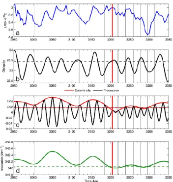
Fig. 7. Orbital variations between 2.950 and 3.350 Ma. (a) the Lisiecki and Raymo (2005) benthic oxygen isotope stack. (b) obliq-uity, with dashed horizontal showing the present-day value, (c) pre-cession and eccentricity, with horizontal dashed black and solid red lines showing present-day values for eccentricity and precession, as derived from the astronomical solution of Laskar et al. (2004; La04). (d) the variation in global mean TOA insolation according to La04, with the dashed horizontal green line denoting the modern value of global mean insolation. The vertical black solid lines and the solid red line through each panel represent the best-fit solutions to the modern orbits as well as the selected initial time slice for in-vestigation discussed in Sect. 6.2 (figure modified from Haywood et al., 2013).
strategy also has the advantage of simplifying the interpre-tation of geological proxies, because palaeo-seasonality has more chance of being the same or very similar to modern seasonality.
The Haywood et al. (2013) recommendation for an initial time slice at 3.205 Ma BP for reconstruction sits in the nor-mal polarity of the Gauss Chron between the Kaena (above) and Mammoth (below) reversals (Fig. 7). The peak deviation in benthic δ18O is centred on Marine Isotope Stage KM5c (or KM5.3). The 0.21 to 0.23 ‰ deviation in δ18O could re-flect a 21 to 23 m sea level rise above modern (assuming 0.1 ‰ equates to ∼ 10 m of sea level rise, Miller et al., 2012), providing that the signal is purely a function of ice volume rather than any change in deep ocean temperatures. Assum-ing the near-total loss of the West Antarctic and Greenland Ice Sheets (a reasonable initial premise given proxy data and model outputs; Naish et al., 2009; Pollard and DeConto, 2009; Dolan et al., 2011; Lunt et al., 2008), volume reduc-tion from the East Antarctic Ice sheet is a moderate 6 or 7 m
of ice volume equivalent. This general interpretation of sea level from the LR04 stack is supported by a recent synthe-sis of sea level records between 2.9 and 3.3 Ma BP by Miller et al. (2012). At ∼ 3.205 Ma BP the Miller et al. (2012) syn-thesis indicates a maximum sea level rise of 25 m ± 5 m (de-rived from Mg/Ca ratios of deep marine ostracods; Dwyer and Chandler, 2009). A mean of multiple sea level records for approximately the same time indicates a peak sea level rise of ∼ 22 m ± 10 m.
During the time slice orbital forcing is close to the mod-ern distribution both seasonally and regionally (Haywood et al., 2013). Additionally, it is preceded by a relatively stable interval (ca. 10 ka) where the insolation distribution is close to modern. During this period, analysis of the insolation pat-terns indicate that it is likely to have been dominated by pro-gressively warmer Southern Hemisphere summers. This is consistent with the benthic δ18O variation seen in the LR04 stack, if ice sheet melt in Antarctica is a primary driver of the
δ18O peak. Available proxy data for atmospheric CO2 (e.g. Bartoli et al., 2011) places an upper limit of ∼ 400 ppmv, with a cluster of four measurements within 100 ka using three different proxy techniques (alkenones, boron isotopes and stomatal density) indicating a range of between 300 to 380 ppmv (Haywood et al., 2013).
7 Conclusions
We present, for the first time, a systematic model inter-comparison and model-data inter-comparison of the results from eleven climate models simulating the mid-Pliocene Warm period. This study includes outputs from atmosphere-only (Experiment 1; including outputs from seven models) as well as coupled atmosphere–ocean climate models (Exper-iment 2; including outputs from eight models). Model results show a range of global mean surface temperature anomalies, even though the models were specified with identical bound-ary conditions. In other words, models respond differently to the forcing derived from Pliocene boundary conditions. For Experiment 2, the range in global annual mean surface air temperature warming is 1.76◦C. For sea surface and sur-face air temperature, the models are least consistent with each other in the North Atlantic and in the high latitudes, respectively. For precipitation they are least consistent with each other in the tropics. Whilst all models predict an en-hancement of the hydrological cycle, the magnitude of this enhancement is variable, and regional disparities in total pre-cipitation are apparent. All models simulate a polar amplifi-cation of surface air temperature warming for the Pliocene, although the magnitude of this amplification is model depen-dant. Our ensembles support previous work suggesting that Earth System Sensitivity (ESS) is greater than Climate Sen-sitivity (CS), and suggest the ratio of ESS to CS is is between 1 and 2.
A. M. Haywood et al.: Results from the Pliocene Model Intercomparison Project 205
Within the ensemble range, the models appear able to re-produce many of the sea surface and surface air temperature anomalies reconstructed from multiple proxies in the South-ern Hemisphere, the tropics, and in the NorthSouth-ern Hemisphere (to ∼ 40◦N). At higher latitudes in the Northern Hemisphere point-to point data/model comparisons indicate that mod-els potentially the magnitude of change on land and in the oceans. Comparison of regional averages highlight Russia and Siberia as particular areas of concern. Whilst these re-sults provide justification for new sensitivity studies specifi-cally targeted towards improving the match between data and models in the higher-latitudes of the Northern Hemisphere, they also highlight the need for reduced uncertainties in tem-perature estimates from geological temtem-perature proxies. We highlight a strategy towards the adoption of more tightly con-strained time slices (Haywood et al., 2013), rather than the current time slab approach, where proxy data may be derived from a window of time as wide as one million years, to help reduce uncertainties in proxy data and the experimental de-sign used in future climate model simulations. Such a com-bined approach will allow for assessments of model perfor-mance for the Pliocene to be made with greater confidence in the future.
Supplementary material related to this article is
available online at: http://www.clim-past.net/9/191/2013/ cp-9-191-2013-supplement.zip.
Acknowledgements. A.M.H., A.M.D. and S.J.P. acknowledge that the research leading to these results has received funding from the European Research Council under the European Union’s Seventh Framework Programme (FP7/2007-2013)/ERC grant agreement no. 278636. A.M.D. acknowledges the UK Natural Environment Research Council for the provision of a Doctoral Training Grant. D.J.H. acknowledges the Leverhulme Trust for the award of an Early Career Fellowship and the National Centre for Atmospheric Research and the British Geological Survey for financial support. C.S. and G.L. received funding through POLMAR and PACES. Z.Z. would like to thank Mats Bentsen, Jerry Tjiputra, Ingo Bethke from Bjerknes Center for Climate Research for the contribution to the development of the NorESM-L. F.J.B. and D.J.L. ac-knowledge NERC grant NE/H006273/1. D.J.L. acac-knowledges Research Councils UK for the award of an RCUK fellowship and the Leverhulme Trust for the award of a Phillip Leverhulme Prize. B.L.O. and N.A.R. recognise that NCAR is sponsored by the US National Science Foundation (NSF) and computing resources were provided by the Climate Simulation Laboratory at NCAR’s Computational and Information Systems Laboratory (CISL), sponsored by the NSF and other agencies. The source code of MRI model is provided by S. Yukimoto, O. Arakawa, and A. Kitoh in Meteorological Research Institute, Japan. Funding for L.S. and M.C. provided by NSF Grant ATM0323516 and NASA Grant NNX10AU63A. W.-L.C. and A.A.-O. would like to thank R. Ohgaito for help in setting up the MIROC4m experiments which were run on the Earth Simulator at JAMSTEC. H.J.D. thanks the
US Geological Survey Climate and Land Use Change Research and Development Program and the John Wesley Powell Center for Analysis and Synthesis. U.S. and A.M.H. acknowledge funding received from the Natural Environment Research Council (NERC Grant NE/I016287/1, and NE/G009112/1 along with D.J.L). The HadCM3 simulations were carried out using the computational facilities of the Advanced Computing Research Centre, University of Bristol – http://www.bris.ac.uk/acrc/.
Edited by: C. Brierley
References
Bartoli, G., H¨onisch, B., and Zeebe, R. E.: Atmospheric CO2 decline during the Pliocene intensification of North-ern Hemisphere glaciations, Paleoceanography, 26, PA4213, doi:10.1029/2010PA002055, 2011.
Bonan, G. B., Oleson, K. W., Vertenstein, M., Levis, S., Zeng, X., Dai, Y., Dickinson, R. E., and Yang, Z.-L.: The land surface cli-matology of the Community Land Model coupled to the NCAR Community Climate Model, J. Climate, 15, 3123–3149, 2002. Braconnot, P., Otto-Bliesner, B., Harrison, S., Joussaume, S.,
Pe-terchmitt, J.-Y., Abe-Ouchi, A., Crucifix, M., Driesschaert, E., Fichefet, Th., Hewitt, C. D., Kageyama, M., Kitoh, A., Laˆın´e, A., Loutre, M.-F., Marti, O., Merkel, U., Ramstein, G., Valdes, P., Weber, S. L., Yu, Y., and Zhao, Y.: Results of PMIP2 coupled simulations of the Mid-Holocene and Last Glacial Maximum – Part 1: experiments and large-scale features, Clim. Past, 3, 261– 277, doi:10.5194/cp-3-261-2007, 2007.
Bragg, F. J., Lunt, D. J., and Haywood, A. M.: Mid-Pliocene cli-mate modelled using the UK Hadley Centre Model: PlioMIP Experiments 1 and 2, Geosci. Model Dev., 5, 1109–1125, doi:10.5194/gmd-5-1109-2012, 2012.
Cattle, H. and Crossley, J.: Modelling arctic climate change, Philos. T. Roy. Soc. A, 352, 201–213, 1995.
Chan, W.-L., Abe-Ouchi, A., and Ohgaito, R.: Simulating the mid-Pliocene climate with the MIROC general circulation model: experimental design and initial results, Geosci. Model Dev., 4, 1035–1049, doi:10.5194/gmd-4-1035-2011, 2011.
Chandler, M., Rind, D., and Thompson, R.: Joint investigations of the middle Pliocene climate II: GISS GCM Northern Hemisphere results, Global Planet. Change, 9, 197–219, 1994.
Chandler, M. A., Sohl, L. E., Jonas, J. A., and Dowsett, H. J.: Simu-lations of the Mid-Pliocene Warm Period using the NASA/GISS ModelE2-R Earth System Model, Geosci. Model Dev. Discuss., 5, 2811–2842, doi:10.5194/gmdd-5-2811-2012, 2012.
Charney, J. G.: Carbon Dioxide and Climate: A Scientific Assess-ment, National Academy of Science, Washington, DC, 22 pp., 1979.
Collins, W. D., Rasch, P. J., Boville, B. A., Hack, J. J., McCaa, J. R., Williamson, D. L., Kiehl, J. T., and Briegleb, B.: Descrip-tion of the NCAR Community Atmosphere Model (CAM3.0), NCAR Tech. Note NCAR/TN-464+STR, National Center for Atmospheric Research, Boulder, Colorado, 226 pp., 2004. Contoux, C., Ramstein, G., and Jost, A.: Modelling the
mid-Pliocene Warm Period climate with the IPSL coupled model and its atmospheric component LMDZ5A, Geosci. Model Dev., 5, 903–917, doi:10.5194/gmd-5-903-2012, 2012.