Dynamic magnetic resonance spectroscopy of phosphate energetics during muscle exercise and recovery

Dynamic magnetic resonance spectroscopy of phosphate energetics during muscle exercise and recovery

par Bahare Sabouri

Département Institut de Génie Biomédical, Université de Montréal Faculté des arts et des sciences

Mémoire présenté à la Faculté des études supérieures en vue de l’obtention du grade de Maître ès sciences (M.Sc.)

en Génie Biomédical

December, 2014

c

Université de Montréal Faculté des études supérieures

Ce mémoire intitulé:

Dynamic magnetic resonance spectroscopy of phosphate energetics during muscle exercise and recovery

présenté par: Bahare Sabouri

a été évalué par un jury composé des personnes suivantes: Gilles Beaudoin, président-rapporteur

Richard Hoge, directeur de recherche Hélène Girouard, membre du jury

L’importance des échanges de phosphore liés à l’apparition de troubles et de mala-dies neurodégénèratives a suscité l’intérêt des chercheurs en ce qui concerne le déve-loppement de technologies pouvant détecter ces composés métaboliques. Á l’aide de la spectroscopie en résonance magnétique du phosphore, il est possible de détecter ces mé-tabolites d’une manière non-invasive. Cette technique permet plus particulièrement de mesurer le taux de degénération de la phosphocréatine (PCr) lors de périodes d’exercice et de récupération post-activité.

Cette dernière métrique agit en tant qu’indicateur valide du métabolisme oxydatif mi-tochondrial dans le muscle et permet de différentier un muscle sain d’un muscle patholo-gique. Pour effectuer l’imagerie ou la spectroscopie par résonance magnétique, de nom-breux outils cliniques peuvent être utilisés afin de générer des images comprenant une variété de contrastes anatomiques et fonctionnels. Par contre, ces contrastes ne peuvent être habituellement produits qu’à partir des molécules d’eau ou des atomes d’hydro-gène renfermés dans les tissus biologiques et les outils permettant de générer les images correspondantes demeurent, pour la plupart, insensibles à la présence d’autres atomes d’intérêt.

Au cours de ce projet, il a été question d’obtenir un spectre du phosphore à partir de l’activité musculaire chez l’humain in vivo en se servant de la technique de spectro-scopie de type31P. Pour ce faire, une antenne radiofréquence à deux canaux, devant être syntonisée à la fréquence de résonance du phosphore, a d’abord été conçue et fabriquée en laboratoire pour ensuite être validée lors d’expériences sur une plateforme IRM 3T de marque Siemens. Les spectres du phosphore furent acquis sur un fantôme, une solution de phosphate de potassium à une concentration de 100 mM, ainsi que sur le mollet d’un sujet humain au cours d’une période de repos, d’exercice et de récupération. Le spectre obtenu à la suite de cette dernière expérience démontre la présence accrue du phosphore lors de procédés métaboliques à haute teneur énergétique impliquant la dégradation de phosphates. Par la suite, il a été question d’observer la variation des niveaux de PCr du-rant des périodes d’exercice et de récupération chez 5 jeunes adultes effectuant une série

iv de flexions plantaires ayant un élément résistif attaché à leurs pieds.

La démarche entreprise au cours de ce projet permettra l’utilisation future des tech-niques quantitatives en spectroscopie pour l’évaluation du métabolisme des phosphates chez des patients souffrant de maladies coronariennes ainsi que chez des sujets contrôles sains provenant du même ensemble démographique.

Entailing of phosphorus exchanges in most bio-chemicals as a key factor in dis-ease, increases researcher’s interest to develop the technologies capable of detecting this metabolite. Phosphorus magnetic resonance spectroscopy is able to detect key metabo-lites in a non-invasive manner. Particularly, it offers the ability to measure the dynamic rate of phosphocreatine(PCr) degeneration through the exercise and recovery. This met-ric as a valid indication of mitochondrial oxidative metabolism in muscle, differentiate between normal and pathological state.

To do magnetic resonance imaging and spectroscopy, clinical research tools provide a wide variety of anatomical and functional contrasts, however they are typically restricted to the tissues containing water or hydrogen atoms and they are still blind to the bio-chemicals of other atoms of interests.

Through this project we intended to obtain the phosphorus spectrum in human body – specificadenerativelly in muscle – using 31P spectroscopy. To do so a double loop RF surface coil, tuned to phosphorus frequency, is designed and fabricated using bench work facilities and then validated through in vitro spectroscopy using 3 Tesla Siemens scanner.

We acquired in vitro as well as in vivo phosphorus spectrum in a 100 mM potas-sium phosphate phantom and human calf muscle in rest-exercise-recovery phase in a 3T MR scanner. The spectrum demonstrates the main constituent in high-energy phosphate metabolism. We also observed the dynamic variation of PCr for five young healthy sub-jects who performed planter flexions using resistance band during exercise and recovery. The took steps in this project pave the way for future application of spectroscopic quantification of phosphate metabolism in patients affected by carotid artery disease as well as in age-matched control subjects.

CONTENTS RÉSUMÉ . . . iii ABSTRACT . . . v CONTENTS . . . vi LIST OF TABLES . . . ix LIST OF FIGURES . . . x

LIST OF APPENDICES . . . xiii

LIST OF ABBREVIATIONS . . . xiv

NOTATION . . . xv

DEDICATION . . . xvi

ACKNOWLEDGMENTS . . . xvii

PREFACE . . . xviii

CHAPTER 1: INTRODUCTION . . . 1

1.1 Magnetic resonance (MR) physics . . . 1

1.1.1 Classical description . . . 1

1.1.2 Quantum description . . . 3

1.1.3 NMR signal detection . . . 4

1.1.4 Bloch equation and bulk magnetization . . . 6

1.1.5 Fourier Transform . . . 7

1.1.6 Resolution enhancement and SNR improvement . . . 9

1.1.7 Chemical shift . . . 10

1.2 Inside the MR . . . 12

1.2.1 Single voxel spectroscopy . . . 12

1.2.2 PRESS (point resolved single voxel spectroscopy) . . . 12

1.2.3 STEAM . . . 13 1.2.4 CSI . . . 13 1.2.5 FID . . . 14 1.3 Energy in Muscle . . . 14 1.3.1 Why phosphorus? . . . 15 1.3.2 Identification of resonance . . . 15 1.3.3 Intracellular pH . . . 16

1.3.4 The phosphagen system in muscle . . . 18

1.3.5 Calf muscle . . . 20 1.4 RF Coil . . . 20 1.4.1 Transmission line . . . 22 1.4.2 RLC circuit . . . 24 1.4.3 Impedance matching . . . 26 CHAPTER 2: METHOD . . . 28 2.1 Coil construction . . . 28 2.1.1 Receiver . . . 28 2.1.2 Transmitter . . . 31 2.1.3 Detuning . . . 32 2.2 Coil fabrication . . . 32 2.3 Bench measurement . . . 34 2.4 Voltage calibration . . . 35 2.5 Depth of penetration . . . 36 2.6 In vitrospectroscopy . . . 37 2.6.1 Phantom . . . 37

2.6.2 Positioning in the scanner . . . 38

viii

CHAPTER 3: RESULTS AND DISCUSSION . . . 42

3.1 In vivo . . . 42

3.1.1 Experimental protocol . . . 42

3.1.2 Exercise protocol . . . 42

3.1.3 Phosphorus MRS protocol . . . 43

3.2 Peak fitting in jMRUI . . . 46

CHAPTER 4: CONCLUSION AND FUTURE DIRECTION . . . 48

4.1 Overview of work . . . 48

4.2 Experimental setup . . . 49

4.3 Existing defects and future works . . . 49

1.I Chemical shift of31P containing metabolites. . . 17 2.I Isolation between tuned and detuned loop . . . 35

LIST OF FIGURES

1.1 Zeeman splitting; energy level for a nucleus with spin quantum

number of 1/2 . . . 4

1.2 Magnetization Mzis flipped by angle alpha using the field B1. The left frame describes the motion of the nuclei by a nutation around the z axis. In the right frame of reference the x,y plane is rotating at ω0 and magnetization, in this example, is seen as tipping along the y’ axis. . . 6

1.3 Exponential decay of the magnetization in transversal plane and its relation with Fourier transform, Figure taken from [1] . . . 8

1.4 Components of a NMR spectrum; the non-zero initial phase of the FID induces the absorption and dispersion components, Figure taken from [1]. . . 8

1.5 Elimination of dispersion part by phase correction, Figure taken from [1]. . . 9

1.6 The peak splitting of the1H due to the J-coupling with13C, Figure taken from [1]. . . 11

1.7 Principal of volume selection . . . 13

1.8 PRESS pulse sequence . . . 13

1.9 STEAM pulse sequence . . . 14

1.10 31P spectrum of a human calf muscle acquired within 3T magnetic field represented in ppm scale, Figure taken from [2]. . . 16

1.11 Displacement of the physiological 31P containing metabolites by pH variation, Figure taken from [2]. . . 17

1.12 The top shows the 31P NMR spectrum of muscle at resting state, muscle at near complete PCr depletion, and muscle with complete PCr depletion, Figure taken from [2]. . . 19

1.13 Axial view of the calf muscle using 3T Siemens MR scanner, im-age taken during study. . . 20

1.14 Magnetic field of a loop. . . 22

1.15 RF signal wave length and the coax length. . . 22

1.16 Signal propagation in inside a transmission line [2]. . . 23

1.17 Network analyzer ports. . . 24

1.18 Highest power transmission at Larmour frequency. . . 26

1.19 Smith chart. . . 27

2.1 RLC circuit of the receive loop. . . 29

2.2 RLC circuit of the transmit loop, detuning and matching circuit of it. 31 2.3 Up: Three dimensional sketch of the box to support the coil. Down: 1Tx-1Rx Rf surface for31P spectroscopy. . . 33

2.4 S11 measurements of each loop; Right: Receiver, Left: Transmitter. 35 2.5 Voltage variation profile of 100mM phantom. . . 36

2.6 In vitrospectroscopy. . . 37

2.7 Proton image of the phantom. . . 38

2.8 Localized automated shim illustration of human calf muscle. . . . 39

2.9 Single voxel spectrum of the 100mM phantom. . . 40

2.10 Spectral map generated by 3D CSI measurement. . . 40

2.11 Time profile of the 3D CSI measurement. . . 41

2.12 Flash image of the phantom in axial view. . . 41

3.1 In vivospectroscopy. . . 43

3.2 Spectrum of human calf muscle in resting state, 256 average, TR of 2000, fid sequence. . . 44

3.3 First subject, exercise protocol: 2-minute resting period, 6 minutes of exercise and a 4-minute recovery period, TR of 2000, 64 aver-ages, fid sequence. Blue parts of the figure indicate the subject is exercising and the black parts belongs to resting and recovery periods. . . 45

xii 3.4 Seconds subject, exercise protocol: 1 minute rest, three blocks of

4-minute exercise period followed by 1 minute pause and 6 min-utes of recovery, 8 averages and TR of 2000 using fid sequence

. . . 45 3.5 Forth subject, exercise protocol: 1 minute of rest, 12 minutes of

exercise and a 6-minute recovery period, 32 averages and TR of

1000 using fid sequence. . . 46 3.6 Curve fitting of 31P spectrum using AMARES and prior

LIST OF ABBREVIATIONS

AD Alzheimer’s Disease ATP Adenosine Tri Phosphate ADP Adenosine Di Phosphate

FID Free induction decay mM milli-Molar

MRI Magnetic Resonance Imaging MRS Magnetic Resonance Spectroscopy

NF Noise factor

NMR Nuclear Magnetic Resonance PCr Phosphocreatine

Pi Inorganic Phosphate RF Radio Frequency ROI Region Of Interest SNR Signal to Noise Ratio SAR Specific Absorption Rate

T1 Longitudinal relaxation time T2 Transverse relaxation time TE Time for Echo

γ Gyro magnetic ratio ν Larmour frequency M Magnetization vector i, j √−1 σ Shielding factor δ Chemical shift B Magnetic field λ Wave length

I would like to thank our funding agencies, CFI and CIHR that have provided the resources necessary to fund this project. This project is above all a collaboration between the LINeV laboratory and the CHUM who made possible a research agreement with Siemens.

I wish to thank my principal supervisor Rick Hoge for all his support and encourage-ment throughout the project. An special thanks goes to Gilles Beaudoin from CHUM. His advice greatly contributed to this project.

Thanks to Raphaël Paquin, from Siemens and Jamie Near, from CIC at Douglas Institute for their consultation.

To my friends and colleagues from LINeV, Isabelle Lajoie, Anne-Marie Bédard, Scott Nugent, Marius Tuznik, Lucile Sink and Kenneth Dyson. Thank you for all the great and the not so good moments and your companionship during the long days. You are an incredible resource that I will greatly miss.

To the UNF that have trained me, Carollyn Hurst and André Cyr, thank you for your help, discussions and spending so much time with me.

And of course, I would like to thank the most important people in my life, my mother Pooran and my sister Sepideh, I couldn’t be here without your help. Thank you for all of your sacrifices and your unwavering support.

PREFACE

There is a growing demand for non-invasive techniques to assess the tissue metabolism and function. Such techniques propose alternatives for determining tissue properties in the normal state and changes in the disease state [3]. Among human diseases affect-ing skeletal muscle; the prevalence of type 2 diabetes in the youth and pressure sore among the elderly is increasing rapidly. The development of technologies to diagnose such disorders will greatly contribute to the management of their prevalence [4].

Among all the image modalities, positron emission tomography (PET) and mag-netic resonance spectroscopy (MRS) are the gold standards when it comes to measuring metabolism [5]. However, MRS offers the non-invasive alternative that is free of the radiation, [6]. Most scanners used in hospitals and research centers are tuned to im-age protons. In contrast, tissue metabolism is based on the exchange of phosphorus metabolism [7].

This project mainly concerns spectroscopic quantification of phosphocreatine metabolism in the muscle of healthy young subjects [8]. Most31P NMR studies are conducted in hu-man muscle due to the high concentrations of phosphorus in this area [9].

The main objective of this project concerns the dynamic measurement of phospho-creatine in human skeletal muscle when the calf muscle goes through exercise and recov-ery period. To achieve this goal we chose nuclear magnetic resonance spectroscopy tech-nique, particularly31P NMR. We are aiming to reach a level of sensitivity in the spec-trum that accurately projects the phosphocreatine depletion and replenishment. Other than that, the resting state spectrum should clearly demonstrate the main constituent of the phosphorus spectrum –including PCr, ATPs and inorganic phosphate–of the skele-tal muscle. Various techniques and hardware were developed for phosphorus imaging on 3 Tesla MRI scanner. In the first phase of the project we develop efficient analysis tools to acquire and quantify phosphorus components. The next step was to optimize the hardware, which is essential for accurate quantification. Finally, the optimized hardware was used to probe the role of phosphorus in biological components, such as adenosine triphosphate (ATP) and phosphocreatine (PCr) in healthy subjects undergoing a

func-tional task.

Hardware aspects of the project included the development of an RF coil. Tests of the hardware were achieved using a double loop coil tuned to the phosphorus resonate frequency on phantoms containing various concentrations of inorganic phosphate. Then the hardware was used to run the experiments on the calf muscle of human subjects. It has been shown through the experiments that the acquired signal in this area gives a robust signal of PCr during contraction exercise and recovery.

Our lab is well experienced in quantitative neuroimaging. Phosphorus spectroscopy is used for the study of phosphorus components in cardiac ischemia and mitochondrial dysfunction in Alzheimer’s disease [10]. The early stage of Alzheimer’s disease (AD) demonstrates a metabolic alteration [7], [11]. Measurement and monitoring of these al-terations are a growing interest among researchers. They have an essential role in the understanding and prevention of mild cognitive impairment (MCI) and the progression to AD [12]. Diagnostics using traditional magnetic resonance imaging (MRI) involves various challenges. Proton magnetic resonance spectroscopy1H NMR can help to iden-tify hydrogenated components of interest. However, this method is still blind to most bio-chemicals involved in phosphorus exchanges of oxidative metabolism.

In the future, the RF coil will be modified to be applicable for use on the brain. Phosphorus metabolism changes will be observed in the healthy brain while doing a functional task. This project has high potential to provide valuable quantitative infor-mation about energy metabolism which helps the understanding of pathophysiology in neurodegenerative diseases.

CHAPTER 1

INTRODUCTION

Molecular medicine has benefited profoundly from nuclear magnetic resonance (NMR) spectroscopy. The development of high field strength magnets and increased accessibil-ity to whole-body scanners for magnetic resonance (MR) imaging initiated the motiva-tion to use non-proton spectroscopy as a diagnostic tool. Among common nuclei with NMR capability,31P and13C are of particular interest. 13C exists in organic compounds and is extensively associated with topics such as glucose labeling. 31P comprises 100% of phosphorus content in the human body and plays a key role in ischemic cardiac my-opathy diagnosis [13], [14], various brain diseases [15] and in the examination of can-cer treatment effectiveness [16], [17]. Among the phosphorus metabolites, adenosine triphosphate (ATP) and phosphocreatine (PCr) are responsible for the regulation of cel-lular energy delivery and responding to changes in muscular tissue energy demand [18]. Recent advances in spectroscopy techniques and equipment have paved the way for the in vivostudy of animal and human biological samples.

1.1 Magnetic resonance (MR) physics

NMR is based on the principals of nuclei spins subjected to a strong static magnetic field and their reaction based on their chemical environment [19]. Specificities concern-ing the physics of spins is a complicated topic, which is not the concern of this thesis. To understand the concept of NMR we first have to acknowledge the nuclear behavior of the spins within a magnetic field. This can be presented as two main perspectives: classical and quantum.

1.1.1 Classical description

The proton can be seen as a rotating object with an electrical charge that is placed in a magnetic field. This will result in the generation of an angular and magnetic

mo-ment. Conceptually, momentum is the tendency for a proton to continue its motion indefinitely. The relationship between magnetic and angular moment is a nuclear spe-cific constant that makes two quantities equal Eq. 1.1 (γ is the gyro magnetic ratio). Hydrogen is the simplest molecule with one positive charge, referred to as a proton. The magnetic moment is as small as 1.4102 × 10−26 JT−1 and the gyro magnetic ratio is

γ

2π = 42.575 MHz

T

µ = γ L (1.1)

Where µ is the magnetic moment and L is the angular moment.

In the absence of an external magnetic field, protons align randomly. When they are subjected to a static magnetic field, B0, protons will start to precess about B0 and are

influenced by a torque given by Eq. 1.2. Torque causes the angular moment changes as Eq. 1.3.

T = µB0 (1.2)

T = dL

dt (1.3)

Combining all the former equations gives dµ

dt = γ µB0 (1.4)

Alternatively the rotation of µ around B0can be expressed as:

dµ

dt = µω0 (1.5)

Combining Eq. 1.4 and Eq. 1.5 gives the Larmor equation and Larmor frequency respectively

3 ν0= ω0 2π = γ 2π B0 (1.7)

The Larmor frequency is proportional to the strength of B0as well as gyro magnetic

ratio – the characteristic of the nucleus. On the other hand, once a particle interacts with the magnetic moment in B0this results in the magnetic energy, defined byµ:

E = −µµµ . B0= −µ B0cosθ (1.8)

θ is the angle between B0and the magnetic moment µµµ . The classical view gives an

idea about how magnetic energy relates to the magnetic moment and the static magnetic field. Quantum description in next section provides a picture about the interaction of nuclear spins and electromagnetic waves.

1.1.2 Quantum description

Considering Eq. 1.1, magnetic moment and angular momentums of elementary par-ticles are parallel vectors and they may be given as

µz= γ(

h

2π)m (1.9)

where m depends on the spin quantum number, I, can have 2I + 1 values, m = I, I − 1, I − 2, ... − I. In an external magnetic field the particle acquires energy given by Eq. 1.8. Considering the quantum description of magnetic and magnetic energy given by the classical view,

E= −µzB0= −γ(

h

2π)mB0 (1.10)

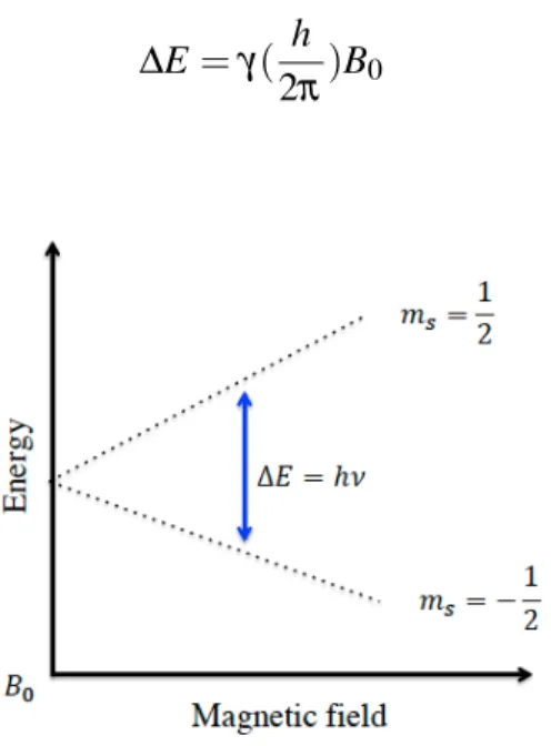
The energy level is quantized due to the discrete value of m and the number of quan-tized energy level in the magnetic field is 2I+1. This means that once a non-zero spin particle is placed in a magnetic field it can take on one of the 2I + 1 levels of energy, for example for I = 1/2 there are two levels of energy (m = −1/2 and 1/2) and the difference between the levels defined as:

∆E = γ ( h

2π)B0 (1.11)

Figure 1.1 – Zeeman splitting; energy level for a nucleus with spin quantum number of 1/2

The resonance phenomena occurs if an oscillating magnetic field is applied perpen-dicular to µ with a ν0frequency. The energy of this magnetic wave is given by Eq. 1.11

and could be rewritten as:

∆E = hν0 (1.12)

Thus the Larmor frequency is given by

ν0= (

γ

2π)B0 (1.13)

Although Eq. 1.13 and Eq. 1.7 yield the same result, quantum and classic descrip-tions are two different approaches for understanding the resonance phenomena for NMR.

1.1.3 NMR signal detection

The longitudinal magnetization, Mz has to be dephased from the z axis and tipped

5 pulsed electromagnetic field, B1, perpendicular to the main magnetic field B0 that flips

the longitudinal magnetization, Mz, at the resonance frequency ν0. This consequently

increases the transversal magnetization, Mxy. A coil perpendicular to B0 generates the

B1 field, which applies a torque to the nuclear spins and tips ~M by the angle α. This

phenomena has been shown on Figure 1.2 on a Bloch sphere and also in a rotating frame when the x-y plane rotates at the Larmor frequency. Normally B1is applied through the

RF pulses and the strength of the torque depends on the RF pulse duration and the mag-netization and M, continues to tip away as long as B1 exists. In fact the magnetization

vector starts processing once it has a nonzero component in the transverse plane. This results in a local magnetic field (B) varying in time. This precessing component is like a small magnet and when it spins inside the loop coil circuit it causes the magnetic flux projected through the loop to vary with time [20].

dM dt ∝

dB

dt (1.14)

This then induces an EMF as per Faraday’s law. The voltage (emf) induced in the de-tector coil is proportional to the rate of change of the magnetic flux in the coil, which in turn is proportional to the rate of change of the oscillating transverse magnetization. We already learned that Larmor frequency is field dependent, Eq. 1.7 and the nuclei will absorb the most amount of energy at this frequency. With an RF pulse that meets the resonance condition, the magnetization vector tips away from the z axis with a preces-sional frequency ω1. Knowing that the magnetic field in the transversal plane is B1we

will have:

ω1= γB1 (1.15)

The receiver coil is sensitive to the transversal magnetization so it detects the most of signal when α is 90 degrees and normally a train of pulses has to be applied to efficiently detect NMR signal.

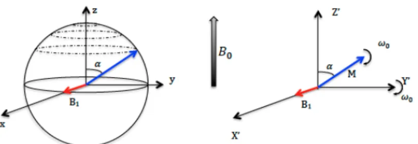
Figure 1.2 – Magnetization Mzis flipped by angle alpha using the field B1. The left frame

describes the motion of the nuclei by a nutation around the z axis. In the right frame of reference the x,y plane is rotating at ω0 and magnetization, in this example, is seen as

tipping along the y’ axis.

1.1.4 Bloch equation and bulk magnetization

By tipping the−→M, the resultant vector is broken into two components: Mxytransverse

and Mz longitudinal magnetization. The longitudinal component returns to its initial

state and the transverse component decays; this phenomenon called relaxation. Bloch equation describes the dynamic process which the relaxation occurs. Components of the−→M, including (Mx,y and Mz), return to equilibrium through an exponential variation.

The transverse relaxation time for Mx,y differs from the longitudinal relaxation Mz. The

relaxation process of the longitudinal, also called spin-lattice, can be written as: dM_z

dt =

(M0− Mz)

T₁ (1.16)

The solution to the differential equation could be written as:

Mz= M0+ (Mz(0) − M0)e−

t

T1 _(1.17)

T1 is the longitudinal relaxation, which describes the time that it takes for the

lon-gitudinal magnetization to return to equilibrium. During this process the spins energy transfers to the lattice.

The other relaxation, called transverse or spin-spin relaxation, explains the net mag-netization decay in the transversal plane from one spin energy level to the other. Equation

7 for this relaxation is:

(dMx) dt = − Mx T₂ + γMyB0 (1.18) (dMy) dt = − My T₂ + γMxB0 (1.19)

Solutions for Mxand Myare:

M_x(t) = [Mx(0)cos(γB0t) − My(0)sin(γB0t)]exp−t/T 2 (1.20)

My(t) = [−M_x(0)sin(γB0t) + My(0)cos(γB0t)]exp−t/T 2 (1.21)

T2 is the spin-spin or transverse relaxation time constant. The spins exchange energy

between themselves, which results in different rates of spin precession, which decreases the phase coherence. T1and T2are both time constants that differs from one material to

another.

1.1.5 Fourier Transform

The RF pulse is calibrated such that it rotates −→M by 90 degrees and positions the magnetization in the transverse plane of the rotating frame of reference, Figure 1.2. At this point magnetization precesses about B0 at the Larmor frequency and induces an

electromotive force, emf, in the receiving coil located in the transverse plane. However, transverse magnetization as well as emf decreases in the form of an exponential decay due to T2relaxation. The acquired signal in the time domain for a sample is represented

as: M_xy= Mxy(0)e−t/T2 Z eiγ∆B0(r)t_{dr= M} xy(0)e−t/T ∗ 2 _(1.22)

∆B0 represents B0 inhomogeneity and equals equals (B0(r) − B(0,nom)). B0(r) the

magnetic field strength, B_(0,nom)the nominal magnetic field strength and Mxyis the

trans-verse magnetization. Emf in time domain, called free induction decay, and magnetiza-tion in the transversal plane has a complex momagnetiza-tion as shown Figure 1.3. The projecmagnetiza-tion vector onto (Mx,t) corresponds to the real portion of Mx,y, while (My,t) corresponds to

Figure 1.3 – Exponential decay of the magnetization in transversal plane and its relation with Fourier transform, Figure taken from [1]

The NMR signal is a signal in complex domain which includes x and y components. The time domain data is rarely used in NMR spectroscopy despite the fact that it provides information about the nuclear spins and resonance frequency. The time domain signal may be converted to the frequency domain using a Fourier transformation. A first di-mension Fourier transformation of the signal represents the frequency component. The real and imaginary parts of the frequency component represent absorption and disper-sion elements –due to the non-zero initial phase of the FID signal. Components of the Lorentzian function are typically used to demonstrate the spectrum.

Figure 1.4 – Components of a NMR spectrum; the non-zero initial phase of the FID induces the absorption and dispersion components, Figure taken from [1].

9 absorption component. Phase correction of the spectrum eliminates the dispersion part leaving only absorption. Purely absorptive signals have a narrower base that allows us to differentiate peaks which are very close to each other. This differentiation would be much easier if the spectrum has been phase corrected to hold absorptive signals. For the phase correction we simply could manipulate the real and imaginary part as follow:

Re(∆φ ) = −Im(∆φ = 0)Sin(φ ) + Re(∆φ = 0)cos(φ ) (1.23) Im(∆φ ) = Re(∆φ = 0)Sin(φ ) + Im(∆φ = 0)cos(φ ) (1.24)

Figure 1.5 – Elimination of dispersion part by phase correction, Figure taken from [1].

1.1.6 Resolution enhancement and SNR improvement

Transverse relaxation time T2 of the spins determines the resolution of the spectra. A long transverse relaxation time leads the spins to decay slowly and fast relaxation pro-vides a quickly decaying FID. The the amount of signal which remains towards the end of the FID determines the resolution. Any data manipulation, e.g. multiplying the FID with a increasing exponential (et/x) will improve the resolution. Conversely, the SNR is determined by the amount of signal at the beginning of the FID. Most manipulations that improve resolution lead to a loss in SNR.

1.1.7 Chemical shift

The signal frequency observed in NMR spectroscopy has a direct relationship to the external magnetic field applied to the nucleus. We saw already the resonance frequency is given by:

ν0= (

γ

2π)B0 (1.25)

Based on Eq. 1.25, all the nuclear spins have the same resonance frequency as long as they are positioned in the same magnetic field strength. However, it is not true in reality because the resonance frequency is highly sensitive to the chemical environment of the nucleus. The response of the electrons in the nucleus to the external magnetic field produce a microscopic magnetic field, which is able to change the effective magnetic field [21]. Therefore, the real magnetic field influences the nucleus is as follow:

B= B0(1 − δ ) (1.26)

δ is the shielding factor and for protons is as small as −10−5 and for other nuclei may be less than 10−3. It is dimensionless and expressed in parts per million(ppm). Thus, the resonance frequency may be modified as:

ν = ( γ

2π) B0(1 − δ ) (1.27)

The chemical shift δ is defined as:

δ = ν − νre f νre f

× 106 (1.28)

ν and νre f are the frequency of the compound under investigation and of the

refer-ence compound. The referrefer-ence compound for protons is tetramethylsilane (TMS), which gives zero chemical shift for in vitro spectroscopy and phosphocreatine resonance (0.00 ppm) for brain and muscle31P spectroscopy.

11 1.1.8 J-coupling

Sometimes the peak in the spectrum splits, this phenomena happens when two or more nuclei interact. The nuclei holding magnetic moments generates a magnetic field. The magnetic field directly influences the neighboring spins. This type of interaction is called bipolar coupling, however, the indirect interaction occurs through the electron cloud of the chemical bond and is called J-coupling or spin-spin coupling. If the spins do not interact with each other then the energy equals ∆E = h f . However during j-coupling of nuclei, the energy will be altered by a coupling constant J and. The possible transition energy could be rewritten as:

∆E = h( f ± J/2) (1.29)

The result will be a peak split by J Hz on NMR spectrum. Another piece of infor-mation that J-coupling provides is the inforinfor-mation about the chemical compound, which in in vivo spectroscopy it is not of interest since lots of metabolite might be located in the closed position and knowing the chemical and by that J-coupling could decrease the sensitivity of the detection as it decrease the amplitude of the peak or information could be contaminated by other metabolite. Therefore, it is desired to get J-coupling under control or remove it if possible [22].

Figure 1.6 – The peak splitting of the 1H due to the J-coupling with13C, Figure taken from [1].

1.2 Inside the MR

In vivo and in vitro spectroscopy uses the MR scanner as it requires a sufficiently strong and highly homogeneous magnetic field. Furthermore, specific sequence for spec-troscopic signal acquisition is necessary. Depending on the type of MRS; single voxel spectroscopy, SVS, or chemical shift imaging, CSI, the sequences varies. In SVS, the signal reflects back from a single voxel while in CSI the spectra belongs to the multiple voxels in a projection, on a slice or a volume. Only in the presence of the homogeneous magnetic field a proper analysis – the differences between the metabolite resonance fre-quencies – of the spectrum is reachable otherwise in a heterogeneous magnetic field the resonance frequency dispersion causes the peaks spread or even appear as a noise. Therefore, prior to spectrum acquisition it is necessary to homogenize the region of in-terest through a process called shimming and for the larger ROI it is harder to reach a proper shimming.

1.2.1 Single voxel spectroscopy

In previous section we saw in SVS the spectrum is acquired from a single voxel hence the acquisition is fast. To choose a single voxel three gradients perpendicular to each other (Gx, Gy, Gz) and three selective radio frequency pulses have to be applied so

that their intersection provides the volume of interest, Figure 1.7. The first pulse excites a layer in the sample, the next one picks a row of that layer and the last pulse make the voxel by picking a cube of the row [23].

1.2.2 PRESS (point resolved single voxel spectroscopy)

In point resolved single voxel spectroscopy, PRESS, the first 90 degrees RF pulse is followed by two 180 degrees RF pulses and the voxel emits a spin-echo signal. PRESS refocuses the spin using a 180 degrees RF pulse, Figure 1.8.

13

Figure 1.7 – Principal of volume selection

Figure 1.8 – PRESS pulse sequence 1.2.3 STEAM

Stimulated echo acquisition mode, STEAM, is same as the PRESS sequence but all the RF pulses have 90 degrees flip angle. The delay time between the second and third pulse called mix time, TM, and the echo time is double of the time between the first two pulses. However, The signal amplitude is half of the PREESS thus the SNR is half of the PRESS, Figure 1.9.

1.2.4 CSI

Chemical shift imaging acquires data from a group of voxels and works base on the repetition of the PRESS and STEAM sequence accompanied by spatial phase encoding so that the spatial location is phase encoded and spectra is recorded for each phase

en-Figure 1.9 – STEAM pulse sequence

coded part. The number of phase encoding pulses as well as their direction depends on the dimension of the interest. For larger number of dimension, the acquisition time will be longer. So the duration time of the sequence is as follow:

t_acq= TR N p1D N p2D N p3D NSA

NSA is the number of signal averages and N pnDrepresents the number of phase

encod-ing steps in direction x.

1.2.5 FID

The FID sequence is unlocalized sequence; it collects the signal from all around the sample that is inside of the coil field of view. It is a commonly used sequence in in vivo spectroscopy where the subjects exercise in the scanner.

1.3 Energy in Muscle

Muscles are nourished by the oxygen that lungs capture from the air and nutrients present within the blood stream [24]. During exercise muscles go through a series of relaxation and contraction. ATP is the key factor in contraction as it breaks into ADP and Pi. This split lets the muscle contract during a cycle of attachment and detachment between actin and myosin (regulatory protein in muscles) [25]. On the other hand,

phos-15 phocreatine (PCr) holds high-energy phosphorus bonds and serves as a source of energy which is available on demand. During contraction PCr concentrations decrease to replen-ish ATP. Another alternative is to regenerate ATP from Adenosine diphosphate (ADP) through oxidative phosphorylation using oxygen from the blood stream. Together, the two mechanisms manage the ATP levels to remain constant [26]. When the workload increases, ATP consumption exceeds its regeneration, which leads to a reduction in pH and acidic cramp of the muscle.

1.3.1 Why phosphorus?

According to previous description, PCr and ATP are the essential energy reservoirs in the biological system and their concentrations vary in each organ. PCr in the brain, heart and skeletal muscle is around 5-6, 10 and 33.5 mM while ATP is 3-4, 6 and 10 mM, respectively. Once the concentrations change they may cause various disease conditions, including muscular disorders, heart infraction and tumors [27]. 31P NMR spectroscopy has been used to study precise metabolic mechanisms and detect the signal from these metabolites. The high natural abundance of phosphorus and its sensitivity (7% of proton) provides a high quality spectrum within minutes of acquisition. Using31P NMR all the key metabolites could be detected [28]. In the next section we will study these key metabolites in the human calf muscle.

1.3.2 Identification of resonance

The phosphorus spectrum of the human calf muscle contains a large peak represent-ing phosphocreatine (PCr) followed by three non-equivalent phosphate groups of ATP. To the left side of PCr, a signal from inorganic phosphate (Pi) exists and under encour-aging circumstances signals from phosphomonoesters and phosphodiesters show up as well [29]. As already addressed in Chapter 1, depending on the chemical environment of each compound, the resonance frequency of the nucleus varies. Therefore, the spectrum of the phosphate chemical content of the muscle is its fingerprint. Figure 1.10 shows the resting31P spectrum from human calf muscle.

Figure 1.10 – 31P spectrum of a human calf muscle acquired within 3T magnetic field represented in ppm scale, Figure taken from [2].

For in vivo spectroscopy PCr frequency position is chosen as the chemical reference fre-quency. 0.00 ppm is the assigned chemical shift value. Tabel 1.I gives the chemical shift of the observable nucleus all around the31P spectrum.

A detailed observation of 31P spectrum of skeletal muscle discloses fine detailed information of phosphorus spins. As described in section 1.6, the mutual interaction between nuclear spins could take place between neighboring phosphorus atoms or pro-tons. The peak splitting in γ-ATP, α-ATP and β -ATP is due to the J coupling phenomena [30]. In other words, the phosphate-phosphate spin coupling and proton-phosphate spin coupling reveals itself in phosphomonoesters, phosphodiesters and diphosphodiester.

1.3.3 Intracellular pH

The chemical shift of the metabolite containing phosphorus depends on some physio-logical parameters such as Magnesium concentration and intracellular pH. The variation of the intracellular pH originates from the protonation of the compounds and it alters the chemical environment and consequently the chemical shift of the compounds. As an example, consider a solution holding two different pH values but identical biochemical

17

Table 1.I – Chemical shift of31P containing metabolites. Compound 31P chemical shift (ppm)

Adenosin monophosphate (AMP) 6.33

Adenosin diophosphate (ADP) α -7.05

β -3.09

Adenosin triphosphate (ATP) α -7.52

β -16.26

γ -2.48

Phosphocreatine 0.00

Inorganic phosphoate 5.02

compounds; ATP, PCr and Pi. The effect of the variation of intracellular pH emerges as a observable shift in the peak’s position on the frequency axis, Figure 1.11.

Figure 1.11 – Displacement of the physiological31P containing metabolites by pH vari-ation, Figure taken from [2].

Intracellular pH is related to the pi-PCr shift. Another physiological parameter that is able to change the resonance frequency position is Mg2+. Particularly β -ATP is the one that mostly dependent on Mg2+content [31].

energy. Muscles use this energy to contract based on the [32]:

AT P → ADP + Pi + energy → Muscle contraction (1.30)

ATP together with ADP, AMP(adenosine monophosphate) and Pi are essential fac-tors for muscle cells to function properly. Once concentrations of ATP decrease, cells rapidly develop fatigue – defined as a depletion of ATP turnover through the skeletal muscle – that consequently reduces the ability of muscle to produce power. Fatigue is an important physiological process that prevents ATP from dropping too low, leading to irreversible damage. By ATP reduction, cells start to compensate for the ATP shortage and demands for its increase. Cells regenerate ATP throughout three systems [33]:

— phosphagen system — Glycolytic system

— Mitochondrial respiration . . .

However, the first system, phosphagen, has the largest contribution in terms of the re-generation rate of ATP and its intensity. In the following we will see how the phosphagen system supplies human body metabolism.

1.3.4 The phosphagen system in muscle

The phosphagen system can be expressed in three reactions:

PCr+ ADP + H+→ AT P +Cr Creatine kinase (1.31) ADP+ ADP → AT P + AMP Adenylate kinase (1.32) AMP+ H+ → IMP + NH₄+ AMP daminase (1.33) The first and second reaction, creatine kinase and adenylate kinase, both regenerate ATP, although the majority of the ATP is produced by creatine kinase. The last reaction does not regenerate ATP, however, it is a part of the phosphagen system that shows how AMP converts to IMP(inosine monophosphate). During hard exercise the energy released by the phosphagen system will continue until PCr is considerably reduced. PCr decreases

19 rapidly and depletion may occur within the first 10 seconds of exercise [25]. That is why most of the intense exercise and sports includes some recovery intervals. Research reveals that the recovery time needed for full compensation of PCr may take as long as 5 to 15 minutes [34], [35]. Figure 1.12 shows the PCr concentration in muscle in resting state and its depletion through exercise [26].

Figure 1.12 – The top shows the31P NMR spectrum of muscle at resting state, muscle at near complete PCr depletion, and muscle with complete PCr depletion, Figure taken from [2].

Figure 1.12 demonstrates how PCr depletes during the exercise phase. The first image shows the phosphorus spectra at resting state. In the next stage, PCr is close to complete depletion. In the last spectra PCr is completely depleted. Simultaneously, inorganic phosphate increases and the position of the resonance frequency moves to right – the chemical shift increase – and the pH increases, which leads to muscle acidosis.

1.3.5 Calf muscle

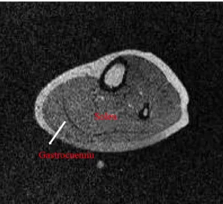
In human body the calf muscle is located on the back of the lower leg and actually consists of two muscles; gastrocnemius and soleus. Gastrocnemius is the largest of the two muscles. The soleus forms the smaller part; a flat muscle positioned beneath the gastrocnemius muscle. The soleus and gastrocnemius muscles are both involved in plantar flexion exercise. We chose calf muscle as a desired organ to conduct 31P spectroscopy, Figure 1.13.

Figure 1.13 – Axial view of the calf muscle using 3T Siemens MR scanner, image taken during study.

1.4 RF Coil

To transmit an oscillating magnetic field and receive the resultant RF signal we have to use a resonator or radio frequency coil –RF coil. During the transmission phase, RF coil terminals receive a high power electrical signal and form a current in the coil conductors. Based on the Faraday’s law this current induces a magnetic field B1 that

oscillates at the RF input frequency. In the receive mode the magnetization vectors inside the sample precess and consequently change the flux within the coil. Once the flux changes – based on Faraday’s law – it induces an electromotive force, emf, in the

21 coil. In fact, the spectrum that we are interested in is this emf, which is amplified and passed through fast Fourier transformation [36].

Surface coils are one of the simplest types of coils able to produce and detect mag-netic fields. Although it is not the most efficient, as the produced magmag-netic field is very inhomogeneous, they are linearly polarized and they can provide higher SNR compared to volume coils because surface coil positions very close to the region of interest, ROI.

Bio-Savart’s law is an analytical model that describes how an electrical current in-duces a magnetic field in a loop. To calculate the magnetic field, a steady current (Idl0) has to be defined and integrated over a closed path of current. The magnetic field can be calculated by:

dB= µ0 4π

I _{I dl}0_{× ˆr}

r2 (1.34)

ris the full displacement vector from the loop element to the field point. ˆr is the unit vector of r, which is the unit displacement vector between the current element and the observation point. For instance, consider a closed loop with the radius of a carrying a constant current I. To calculate the magnetic field of this loop, by Eq. 1.34, the magnetic field sweeps out of the loop and makes a cone, Figure 1.14. The horizontal components of the magnetic field is canceled out and the vertical component adds up to:

B(z) = µ0 4π I _{I dl}0 r2 cos(θ ) (1.35) B(z) = µ0 4π I(2πa) r2 cos(θ ) (1.36)

Given that r2= a2+ z2and cos(θ ) = a/(a2+ z2)1/2

B(z) = µ0I 2

a (a2_{+ z}2₎32

(1.37)

Eq. 1.37 gives the magnetic field at any distance from the loop. The strength of the field decreases as the distance from the center of the coil increases. Based on Lenz’s law any flowing current is capable of creating a magnetic field in the loop. If the current

Figure 1.14 – Magnetic field of a loop.

is applied at the resonance frequency of the coil the induced magnetic field is much stronger. At the resonance frequency the imaginary parts of the impedance of the loop are canceled out and the impedance is pure resistance. The impedance of the coil is calculated by:

Z= jωL + 1

jωC (1.38)

Here L is the inductance of the coil and C is the capacitors on it.

1.4.1 Transmission line

To propagate the signal through the sample and transmit the power between the coil elements, transmission lines are necessary. The transmission line in RF coils are nor-mally coaxial cables that have 50 Ohms impedance. Figure 1.16 shows how a wave

Figure 1.15 – RF signal wave length and the coax length.

propagates within a cable. Once the wave enters a load it divides into two parts; trans-mission and reflection. The transtrans-mission lines ending with their nominal impedance

23 only have a transmission component and do not reflect any portion of the wave back to the source. This is an important fact called matching that we will describe in more detail in section 3.4.

Figure 1.16 – Signal propagation in inside a transmission line [2].

The reflection coefficient describes the amount of the wave reflected back to the source as a ratio of the electric wave voltage and the regressive wave.

Γ =(V+) (V−)

(1.39) The impedance of the load at the end of the transmission line can be defined as

ZL= Z0

V₊(0) +V−(0)

V+(0) −V−(0)

(1.40)

while Z0 is the characteristic transmission line impedance, the reflection coefficient

can be rewritten as Eq. 1.41 that measures the amplitude of the reflected wave compared to the amplitude of the incident wave.

Γ =

Z_charge− Z0

Z_charge+ Z0

(1.41) In fact, the easier way to measure the amount of reflection is using the standing wave ratio, SWR, that measures the maximum voltage to the minimum voltage of the line. The voltage is at a maximum when the incident and reflected waves are in phase and at a minimum when they are out of phase. The equation of SWR can be easily rewritten in

terms of the reflection coefficient. SW R= |V+(0)| + |V−(0)| |V+(0)| − |V−(0)| (1.42) SW R=1 − |Γ| 1 + |Γ| (1.43)

SWR directly describes at which point the line impedance is matched to the load. For those circuits that are perfectly matched, SWR equals one. A network analyzer measures the amount of power reflection and transmission by its scattering ports. The S11 port in

a network analyzer represents the reflection coefficient from the coil. As an example, if S₁₁ = 0 dB it means all the power is reflected back to the source power and no power is radiated to the coil. The larger return loss means the amount of reflection is smaller than the transmission. In surface coils we are aiming to have a S11 parameter of around -20

dB.

Return loss= −20 logΓ = −20 logZload− Z0 Z_load+ Z0

(1.44) Coaxial cable is the most commonly used transmission line. However, they hold

un-Figure 1.17 – Network analyzer ports.

wanted common mode current and also attenuate the signal all along their way to the coil. Common mode currents cause an external coupling between the coils and radia-tion. It has been shown that the shorter length of the cable may reduce the amount of loss and suppress the common mode [37].

1.4.2 RLC circuit

A circuit consisting of resistance, capacitors and inductors could be arranged such that it resonates at a specific frequency. To do so, an RLC circuit should satisfy the

25 equation below, while q is the electric charge flowing in the circuit and induces an emf, E(t): L_t(d 2_q) (dt2₎ + Rt dq dt + q Ct = E(t) (1.45)

solving the second order equation gives:

q(t) = Asin(ω0t+ θ ) (1.46)

while ω0= 1p(LtCt), Rt,Lt and Ct are total resistance, total inductance and total

capacitance, respectively. Normally the Rt is desired to be as low as possible to have the

least loss and Lt is the intrinsic inductance. By choosing the proper capacitors the coil

resonates at the desired frequency [38, Ch. 1, p. 6]. Another approach to acquire reso-nance frequency is the total impedance of the circuit. For an RLC circuit the impedance of each element is R, jωL and 1/ jω C and is dependent on their arrangement; series or parallel. The total impedance of the circuit is given by:

Zt =

∑

_∑

While Yt =_Z1_t and the former equation can be written as

1 Zt =

_∑

In the aforementioned scheme for the31P surface coil, an RLC circuit is in series, so the total impedance will be

Z_a= Rt+ i(ωLt−

1 ωCt

) (1.50)

If the imaginary part is canceled then the coil has the minimum impedance. In other words, the largest current will flow within the coil at the Larmor frequency which is

calculated as Eq. 1.51.

ω0=

1 √

LC (1.51)

Figure 1.18 – Highest power transmission at Larmour frequency.

1.4.3 Impedance matching

The previous section explained how a resonance frequency provides the coil with a pure resistive behavior. However, the exact value of the impedance also depends on the resistance of the target tissue and metabolic constituents. To transfer the energy optimally from the coil to the target tissue (and the other way around) the impedance of the RF coil must be matched to the impedance of the transmission line, which is 50 Ohms. It is not feasible to do impedance matching for each single subject or phantom; instead the impedance matching can be done using a phantom containing the typical constituent of the tissue of interest. Consequently we assume that the coil is in its optimal condition to transmit and receive the RF signal. In the coils that lack a proper matching, a large fraction of the RF power generated will not be transmitted into the target as it should be, instead it will be reflected back at the coil transmission line interface to the power source. In next section we will see how a method called a Smith chart aids us to reach the 50 Ohms matching.

27 1.4.3.1 Smith chart

The Smith chart is the most commonly used graphical chart in RF communication. The calculation is required to observe the mutual conversion between the load impedance and the reflection coefficient. Impedance circles and reactance curves mainly constitute the Smith chart as shown in Figure 1.19. Each load impedance could be shown as a dot on the chart with a specific resistance and reactance.

Figure 1.19 – Smith chart.

As we discussed before, the ideal operation point of the coil is where the load impedance equals the intrinsic impedance of the transmission line, 50 Ohms. At the center of the chart the reflection coefficient is zero as Zload

Z0 equals one. To have the

min-imum reflection the impedance of the load has to reach the center of the chart where the load becomes the real resistance with null reactance.

METHOD

2.1 Coil construction

The growing demand for multi-nuclear NMR spectroscopy along with a proton nu-clei channel for localization and shimming requires non-proton MR probes that perform with high sensitivity. It is more common to use a Tx-Rx switch between transmitter and receiver elements. However, the use of two separate loops, one for transmitter and the other for receiver, allows a free switch coil. This chapter describes different elements of 1Tx-1Rx31P surface coils, including the steps for design, fabrication and validation.

2.1.1 Receiver

A dipole magnetic coil, called a surface coil, is commonly used to receive RF signals. Volume coils also are able to receive RF signals, however, surface coils can be positioned closer to the ROI and provide higher SNR. On the other hand, volume coils benefit from a more homogeneous magnetic field. In cases where an array of the surface coils receive the signal, each element should be decoupled from the others. Otherwise the impedance will consequently change as well as the resonance frequency. To tackle this problem the elements have to be decoupled using geometric decoupling, such that the center of the circular loops should be at the distance of 0.78 times the loop diameter. For the square loops, the distance between the centers is 0.86 times the linear dimension in which the coils are overlapped. At this point the mutual inductance becomes zero.

Considering that the RF coil has two separate loops (transmitter and receiver), to avoid signal interferences the loops must be mutually decoupled. Most of the decoupling strategy uses the active switching of PIN diodes as shown in Figure 2.1. During the transmission of the Tx loop, the diode on the Rx loop has a forward bias; this leads to a

parallel circuit between L and C. This parallel circuit, in cooperation with the loop of the coil, induces a resonance frequency so it resonates in another frequency instead of

29

Figure 2.1 – RLC circuit of the receive loop.

the Larmor frequency. In receive mode the diode is biased reversely so the circuit will be open and the coil will resonate at the desired frequency.

2.1.1.1 Signal to noise ratio, SNR

It has been shown that there are two major sources of noise in MRI [39]. The first one is the eddy current that is magnetically induced in the sample. The second one is the losses due to series inner wire resistance of the receiver coil. Thus the loss function can be formulated as: SNR ∝ ω 2_B 1 √ r_coil+ rsample (2.1) r_coil is the total resistance of the coil and r_samplerepresents the effect of the sample on the receiver coil. In the receiver coil, assuming that a larger transmitter induces a more homogeneous magnetic field, the B1is the principal factor in SNR. For a single loop of

the receiver coil, B1is calculated as

Signal ∝ ω2B1(z, a) ∝

(ω2a2)

(√a2+ z2₎3 (2.2)

The coil sensitivity decreases as the distance from the coil increases and those tissues that are closest to the coil contribute the most to rsample. The effective dimension of

contributing to the loss is given by:

r_sample= ω2f(a) (2.3)

f(a) is a geometry function of the coil radius and by increasing the size of the coil f(a) grows rapidly. That is why smaller coils provide larger SNR. It has been shown that in surface coils, rsamplecan be nine times greater than rcoil. By neglecting the rcoil

SNR is rewritten as

SNR ∝ ω

apf(a) [ a2

(a2_{+ z}2₎3] (2.4)

The first term shows that a larger coil lacks the lower SNR and the second term shows that SNR drops as the distance from the loop increases. Thus, SNR for a surface coil depends more on the coil geometry than the tissue volume.

2.1.1.2 Preamplifier

The received signal from the tissue is very weak so it needs to be amplified on the receiver side. To do so a low noise preamplifier (LNA) tuned to the Larmor frequency, is used (it will be referred to as simply a preamp). The commercial preamplifier, as well as the ones we used, magnifies the signal by factor of 1000, or 30 dB. Other types which amplify by factor of 20 dB are also available.

G(dB) = 10 log Pout put

P_input (2.5)

G(dB) = 10 log 1000 = 30 dB (2.6)

The preamps we used were initially tuned to proton frequency. To make them operate at phosphorus frequency we changed their resonance frequency by adding capacitors and inductors the gain reduced to 25 dB. The noise factor (NF) is calculated by the logarithmic difference of the noise output with the real receiver and noise from an ideal receiver. The commercial preamps have an NF lower than 0.5 dB, which decreases SNR. On the other hand it reduces the amount of noise coming from the transmission line if it

31 is positioned as close as possible to the source.

NF(dB) = 10 log Noiseout put G.Noiseinput

(2.7)

Port S21 on a network analyzer measures the amplification gain such that port S2

trans-mits the signal to the preamp and port S1 receives the amplified signal after it passes

through the preamp. Given that the intrinsic power of the coil is quite low, around µV , using the preamp the power increases to mV .

2.1.2 Transmitter

The transmitter coil inside the MR machine excites the spins in the sample. It induces the B1magnetic field, which disturbs the spins with the desired frequency. The proposed

structure for the transmitter is same as the receiver; a single loop tuned to31P frequency. It has a larger diameter and a matching circuit on the loop. The larger diameter for the transmitter allows us to excite deeper tissues and provide more homogeneous magnetic field for the receiver.

Figure 2.2 – RLC circuit of the transmit loop, detuning and matching circuit of it.

2.1.2.1 SAR calculation

Specific absorption rate (SAR) is the amount of RF power absorbed per unit of sam-ple mass. It describes the vulnerability of the tissue to heating due to RF energy. It is

measured in units of (watts/kilogram). When RF energy is transmitted into the tissue, it causes the ROI to heat. In high enough energy the tissue may be damaged. The SAR value should thus be kept low; for the field strength of the 1.5T, the SAR is quite low and a negligible amount of RF is absorbed by the tissue. However for a 3 Tesla, the higher frequency will increase the absorption of the energy and SAR will be quadrupled. Food and Drug Administration (FDA, USA), has defined SAR limits. It has been suggested that the limit for the MR machine is 3 W/kg averaged over the whole head in 10 min, 4 W/kg averaged over the whole body in 15 min, or 8 W/kg per gram of head/torso tissue in 5 min or 12 W/kg per gram of extremity tissue over 5 min as the normal mode limit [40].

2.1.3 Detuning

Given that transmitter and receiver coils resonate at the same frequency they have to operate independently. Diodes are the principal component in the detuning circuit, so that depending on the bias direction – forward or inverse– allows only one of the loops to operate at a time. The detuning circuits could be positioned anywhere on the loop coil; for the transmitter and receiver we put them as a simple series circuit on the loop. When the diode is forward biased the current circulates only in the detuning circuit and not in the loop, thus the coil resonates in another frequency, which is far from the phosphorus Larmor frequency.

2.2 Coil fabrication

During spectroscopy experiments the coil is positioned under the sample and should withstand the weight. An important aspect of the coil’s design concerns the stability. To prevent any breakage and mis-connection we designed a box and printed precisely. The printer is Elite 3D of the economy size that uses acrylonitrile butadiene styrene (ABS). It is a relatively rigid thermoplastic, resistant to shocks, light-weighted and MR compatible. A box with a curve surface, a wall, a disc and a bottom surface was printed. The parts have been designed with a slide system such that they hold together tightly.

33 The coil has one receiving element that we want to be positioned as close as possible to the target sample. The curved surface of the box, on the top, is located under the sample holder – calf muscle or phantom. Using small screws we attached the receiver element on the under side of the curve surface. The transmitter loop is positioned on the disc as close as possible to the receiver. The PCB board holding the cable traps (to block the proton frequency during31P spectroscopy) and preamp was screwed to the bottom of the box.

Figure 2.3 – Up: Three dimensional sketch of the box to support the coil. Down: 1Tx-1Rx Rf surface for31P spectroscopy.

2.3 Bench measurement

To make sure elements are workings well together, a series of bench measurements needed to be performed.

The receiving and transmitting elements and detuning circuit were individually tuned to 49.8719 MHz. To tune the coil, four capacitors were located on the loop and using the S11 port of the network analyzer we observed the resonance frequency. Given the

capacitors value as well as the resonance frequency we are able to calculate the induc-tance of the loop using Eq. 1.51. Knowing the inducinduc-tance of the loop and the Larmor frequency, the right value of the capacitors could then be calculated to reach the desired frequency. Next, to reach an impedance of 50 Ohms at the end of the transmission line, a parallel circuit of the inductors and capacitor is considered. The impedance was ad-justed by changing the value of the capacitors and inductors of the matching circuit. An example of tuning and matching results obtained for the relative magnitude of the signal and resonance frequency is shown in Figure 2.3. These measurements were taken in S11

mode while one end of the coaxial cable went to the coil and the other was connected to the input terminal of the network analyzer. Considering the preamp already tuned to 50 Ohms we didn’t consider it in matching. The network analyzer should take into account the length of the coaxial cable, so a calibration should be performed with the same cable length prior to tuning and matching. The tuning and matching is performed separately for Rx and Tx.

The following steps must be taken to assure the effectiveness of the detuning circuit. The receiver element should not absorb the RF energy when the transmitter is sending power. The same is true for the transmitter when the receiver is operating. To see the isolation between the loops a S21 measurement is performed using two geometrically

decoupled loops. The probe is placed around the receiving element when it is idle and when it is active mode. The isolation between the transmitter and receiver loop was perfectly achieved and the detuned state for them is shown in Table2.I.

35

Figure 2.4 – S11 measurements of each loop; Right: Receiver, Left: Transmitter. Loop Isolation Tuned Detuned

Transmitter -33 dB 25 dB -18 dB Receiver -33 dB 26 dB -17 dB Table 2.I – Isolation between tuned and detuned loop 2.4 Voltage calibration

Once the setup is perfectly matched and tuned, the MR scanner is used to execute two sets of31P spectroscopy. First, in vitro31P spectroscopy using two phantoms containing different phosphorus concentrations, 10 mM and 100 mM respectively. Second, in vivo

31_{P spectroscopy on the calf muscle of healthy subjects during resting state and during}

exercise. The aim of this chapter is to use MR images and spectra as an indication of coil performance. We will also discuss the methodology and tasks –prior to and during the experiment– required to perform spectroscopy using a 3 Tesla MR scanner.

For the commercial coils, the MR scanner sends a voltage through the transmitter so that the receiver acquires the highest signal intensity from the desired voxel. For the hand-made coils the user has to obtain this optimum voltage manually, or include this task in the pulse sequence for greater efficiency. Therefore, prior to testing the coil on the phantom, or the subject, a voltage calibration needs to be performed. To do so the coil is positioned on the phantom and using a fid sequence the voltage is gradually increased starting from 10 volts up to 200 volts with incremental steps of 10 volts. Through this

Figure 2.5 – Voltage variation profile of 100mM phantom.

procedure TR was quite long and TE was relatively short. We aim to find the smallest

power entry, which provides the largest possible signal and expect a curve that follows a sine wave. The signal intensity increases with voltage increments up to Vopt. This gives

the true 90 degrees excitation. Once excitation exceeds 90 degrees and Vopt is passed,

the signal intensity drops. At 2 × Vopt the flip angle is 180 degrees and the spins stay

in the same direction and absorb enough energy to change from parallel to anti-parallel orientation. For the 100 mM phantom the optimum voltage equals 70 volts and for the rest of the experiments on this phantom we will use this as the reference voltage.

2.5 Depth of penetration

We already saw that the excitation is stronger for tissues closer to the coil. It has been shown that the depth of the penetration for a loop is almost equal to its radius [37]. The transmitter loop with the larger diameter (14.5 cm) excites a slice with thickness of up to 7.25 cm. The receiver (11 cm) collects the signal from the slices, up to 5.5 cm thickness. We chose the smaller receiver to precisely acquire the signals, for the smaller ROI. The dimensions are appropriate for studying various sizes of calf muscle as well as fat thickness across different subjects.

37 2.6 In vitro spectroscopy

Once the bench tests and voltage optimization are successfully performed, to vali-date the hardware and sequences designed for the phosphorus spectroscopy we aim to implement in vitro tests.

2.6.1 Phantom

Phantoms are the main element in in vitro testing. They are especially useful during the SAR calculation, voltage calibration. Also, with prior knowledge of the phantom concentration a quantitative measurement can be performed. The phantoms for the in vitro testing were made based on the recommendations from Provencher [41] –used in proton spectroscopy. A buffer solution containing potassium phosphate and salts pro-vides a total concentration of PO4of 100 mM. To evaluate the coil response in detecting

a phosphorus signal two phantoms are required. One has a higher concentration of phos-phorus metabolites, 100 mM. While the other phantom contained a lower concentration, 10 mM. The low-concentrated phantom was intended to simulate the phosphate concen-tration of the same order of magnitude of the one found in the human body.

2.6.2 Positioning in the scanner

During the phantom test, the curved surface of the coil box which holds the receiver is located under the phantom, as shown in Figure 2.6. Phantoms are preserved in a fridge to prevent any chemical degradation. One hour before testing they are removed to let them reach room temperature.

Figure 2.7 – Proton image of the phantom.

Velcro is used to wrap the coil to the phantom to help prevent movement. To locate the coil coordinates, a small pill is positioned at the center of the receiver. Figure 2.7 shows the anatomical image of the phantom captured by proton imaging. The small white spot represents the pill and consequently the coil location on the phantom. The black space between the pill and the phantom is air bubbles; to avoid them we put small wedges beneath the top of the bottle to help tilt it.

2.6.3 3D Shimming

The next step is to shim the local magnetic field. This homogenizes the magnetic field over the desired area of the volume and obtains the best possible Lorentzian line shape for various resonance peaks over the spectrum. A proper shim provides a FWHM of less than 25 Hz for 3D MRSI. This provides better water suppression, which is crucial in proton spectroscopy as well as a precise peak separation. The resulting field map over the sample is shown in sagittal view. Doing that the system calculates the currents

39 required in the gradient coil to provide the optimal homogeneity over the spectroscopic ROI. Normally a couple of measurements is required to reach optimal shimming.

Figure 2.8 – Localized automated shim illustration of human calf muscle.

Since we intend to run 31P spectroscopy we need to introduce the exact frequency of the desired compound to the MR machine. To do so in the X-frequency section we defined the exact resonance frequency. The Larmor frequency of phosphorus in a 3 Tesla external magnetic field is 51.7 MHz. It is interesting to note that Siemens MR scanners are not exactly 3 Tesla but 2.89 Tesla. This slight difference significantly changes the Larmor frequency. Considering the actual strength field of 2.89 MHz the31P resonance frequency is calculated as follows:

f = γ

2π B = 17.235 × 2.89 = 49.8719 MHz (2.8) Lastly, to have the strongest signal intensity the optimum voltage (section 5.2) needs to be imported as the reference amplitude in the transmitter section. Figure 2.9 demon-strates the phosphorus spectrum of the phantom acquired by the single voxel spec-troscopy sequence. The voxel size was 4 × 4 × 4 cm and TR= 1500 and TE=15 ms.

Data collected was processed in jMRUI and MATLAB. The spectrum shows the real part of the data and underwent phase correction before plotting.

Another sequence provided by Siemens is 3D chemical shift imaging, discussed in section 1.7.4, which acquires the signals from a group of voxels. Without changing the coil place from the previous section the 3D CSI applied. Each single voxel size is