HAL Id: tel-01376744
https://tel.archives-ouvertes.fr/tel-01376744
Submitted on 5 Oct 2016HAL is a multi-disciplinary open access archive for the deposit and dissemination of sci-entific research documents, whether they are pub-lished or not. The documents may come from teaching and research institutions in France or abroad, or from public or private research centers.
L’archive ouverte pluridisciplinaire HAL, est destinée au dépôt et à la diffusion de documents scientifiques de niveau recherche, publiés ou non, émanant des établissements d’enseignement et de recherche français ou étrangers, des laboratoires publics ou privés.
vivo phantom using magnetic resonance elastography
(MRE)
Mashhour Chakouch
To cite this version:
Mashhour Chakouch. Viscoelastic properties of in vivo thigh muscle and in vivo phantom using magnetic resonance elastography (MRE). Biomechanics [physics.med-ph]. Université de Technologie de Compiègne, 2015. English. �NNT : 2015COMP2236�. �tel-01376744�
Par Mashhour CHAKOUCH
Thèse présentée
pour l’obtention du grade
de Docteur de l’UTC
Viscoelastic properties of in vivo thigh muscle and in
vitro phantom using magnetic resonance
elastography (MRE)
Soutenue le 07 décembre 2015
Spécialité : Biomechanics and Bioengineering
1
To obtain the degree of Doctor issued by
Sorbonne University, Université de technologie de Compiègne
Doctoral School « Sciences pour l'Ingénieur »
Disciplinary field: Biomechanics and Bioengineering
Presented and publicly defended by
CHAKOUCH Mashhour
07-12-2015
Jury Member
M. Jean-Marc Constans Centre Hospitalier d’Amiens Reviewer
M. Jean-Michel Franconi Université Bordeaux 2 Reviewer
Mme. Marie-Christine Ho Ba Tho Université de Technologie de Compiègne Examiner M. Fabrice Charleux ACRIM-Polyclinique Saint Côme Examiner
M. Philippe Pouletaut Université de Technologie de Compiègne Examiner
Mme. Sabine Bensamoun Université de Technologie de Compiègne Supervisor
Viscoelastic properties of in vivo thigh muscle and in vitro phantom using
magnetic resonance elastography (MRE)
3
4
Figure 1.1: Types of skeletal muscles ... 21
Figure 1.2: The three types of muscle-tendon arrangement, a) the parallel-fibered muscle, b) the unipennate muscle and c) the bipennate muscle. P.C.S. marks the physiological cross-section that cuts all the fiber. Reprint from Gray's Anatomy (Gray et al., 1924). ... 22
Figure 1.3: Identification of slow and fast fibers, according to Kim and Choi, 2009 ... 23
Figure 1.4: multi scale organization of the muscle system ... 24
Figure 1.5: Sarcomere structure ... 25
Figure 1.6: Axial image with the investigated thigh muscles. Quadriceps muscle (VL: vastus lateralis, VI: vastus intermedius, VM: vastus medialis, RF: rectus femoris), Sr: sartorius, Gr: gracilis, AD: adductor, hamstring muscles (ST: semitendinosus, SM: semimembranosus, BC: long and short biceps) ... 26
Figure 1.7: Schematic representation of muscle architecture. ... 27
Figure 1.8: Mechanical model of muscle Shorten-Hill (1987); CC: Contractile component, PEC: Parallel elastic component, SEC: Series elastic component ... 29
Figure 1.9: Different simplest cases of stresses and strains and their associated tensors (illustrated in 2D) ... 31
Figure 1.10: The principle of incompressibility. The volume of the incompressible object remains constant during (Lindberg, 2013). ... 34
Figure 1.11: Representation of the compression (A) waves and the shear (B) waves. ... 37
Figure 1.12: Variation of the mechanical compression and shear modulus of various biological tissues. Ranges associated with each modulus for a given tissue type are indicated by the shaded regions (Sarvazyan et al., 1998). ... 38
Figure 1.13: Rheological models used in the literature for the characterization of biological tissues.G*isthecomplexshearmodulus,μisshearmodulus,ηisviscosity,fis thefrequencyandωisthepulsation(2.π.f) ... 40
Figure 1.14: a: Custom built for the characterization of mechanical properties of liver (Schwartz et al., 2005). b: Experimental setup high speed cyclic testing rig. (A) Top platen; (B) bottom platen; (C) LVDT transducer; (D) static load cell; (E) dynamic load cell; and (F) connection with shaker (Van Loocke et al., 2009). . 42
Figure 1.15: Experimental setup for testing by indentation(Carter et al., 2001) ... 44
Figure 1.16: 1: the ultrasounds are successively focused at different depths to create pushes by radiation pressure. The constructive interferences of the shear waves form a supersonic Mach cone (in which the speed of the source is greater than the speed of the generated wave) and a quasi-plane shear wave is created; 2: the ultrasound machine then switch into an ultrafast imaging mode to follow the shear wave that is propagating through the medium (Gennisson et al., 2013). . 48
Figure 1.17: Shear waves velocity cartographies, obtained on the biceps brachii and brachialis by Supersonic Shear Imaging technology for different loads (Gennisson et al., 2010). ... 49
5
the medium creating, among others, a shear wave. The ultrasound transducer, which is placed on the vibrator, thus allows following, by axial intercorrelation of the ultrasound speckle and more than one thousand times per second, the propagation of the shear wave depending on the depth over time. We can then deduce the speed of the shearwaveandthustheYoung’smodulusofthemedium (Gennisson et al., 2013). ... 49 Figure 1.19: Comparison between (a) the numerical simulation of the time/depth profile and
(b) the time/depth profile in a muscle in vivo. The slope allows to work back to the speed of the shear wave and thus the Young’s modulus of the medium ( Gennisson, 2003). ... 50 Figure 1.20: The ultrasound array, mounted on a vibrator, gives a low frequency shock in the
medium (around 50 Hz). The shear waves generated on the borders of the array interfere within the imaging plane as a quasi-plane wave propagating on the depth; 2: the ultrasound, then, switches into an ultrafast imaging mode to follow the shear wave , propagating through the medium (Gennisson et al., 2013). .... 51 Figure 1.21: a: breast elastography. An adenocarcinoma appears stiffer in the elasticity
image (Bercoff et al., 2003). ... 51 Figure 1.22: The velocity of the shear wave in a human bicep contracted by various loads. . 52 Figure 1.23: MRE head driver with a loud speaker coupled with a long carbon fiber rod
(Sack et al., 2008). ... 53 Figure 1.24: MRE liver driver with a loud speaker coupled with a plastic air-filled tube
(Talwalkar et al., 2008) ... 54
Figure 1.25: MRE tests composed of a driver (tube) with a loud speaker coupled with a plastic air-filled tube (Bensamoun et al., 2006)... 54 Figure 1.26: Schematic diagram of MRE sequence. Modified extracts (Manduca et al., 2001;
Yin et al., 2007) ... 56 Figure 1.27: Images obtained during an MRE sequence: anatomical image (A) and phase
image (B). The example is taken from a phantom. ... 56 Figure 1.28: Measurment shear modulus (μ, kPa) from the calculation of the wavelength λ
(mm) by placing a profile (red) in the direction of the wave propagation direction on the phase image. ... 57 Figure 1.29: MRE results for normal (35 volunteers) and fibrotic (48 volunteers) livers.
Anatomical images for normal (a) and fibrotic (d) liver. Displacement images for normal (b) and fibrotic (e) liver. Stiffness maps for normal (c) and fibrotic (f) liver. (Yin et al. 2007) ... 61 Figure 1.30: Experimental data for shear moduli (A) and shear viscosity (B) acquired at 25
Hz (circles) and 50 Hz (triangles) wave excitation. The error bars correspond to the standard deviations of the data for each frequency and volunteer (Sack et al., 2008). ... 62 Figure 1.31: A:Principle of the mechanical excitation of shear waves inside the agar gel
6
The wavelength of longitudinal strain waves is long er than that of transverse strain waves. (Oida et al., 2004). ... 67 Figure 1.33: A: Setup of the MRE scan on an agarose gel phantom,B: A superior view of a
MRE wave image for the cylindrical 2% agarose gel phantom at frequency of 150Hz.. I. Round gel phantom in a container, II. The applicator of the electromechanical driver. The diameter of the tip is 10 mm, III. The electromechanical driver which is phase-coupled with oscillating the motion sensitizing gradient, IV. Head coil (Chen et al., 2005b). ... 68 Figure 1.34: Experimental setup for MRE heart phantom (Kolipaka et al., 2009b) ... 68 Figure 1.35: Magnetic Resonance Elastography (MRE) tests performed on a plastic phantom
with a pneumatic driver (Leclerc et al., 2013b). ... 69 Figure 2.1: Manufacturing protocol for plastic phantoms ... 92 Figure 2.2: Fibers orientation ... 93 Figure 2.3: MRI sagittal acquisitions of the thigh muscles (A) (RF: rectus femoris, VI: vastus
intermedius) and (B) the phantom showing similar structures. ... 93 Figure 2.4: Device to stretch the fibers ... 94 Figure 2.5: Set up of the hyper-frequency viscoelastic spectroscopy tests performed on the
different small phantoms ... 95 Figure 2.6: MRE tests performed on the large phantom with two different drivers. ... 96 Figure 2.7: MRE Experimental set-up for the homogeneous phantom (a) (50% plastic). Phase
images showing wave’sdisplacementinsidethephantomsat60Hz(b),80Hz (c) and 100 Hz (d). ... 97 Figure 2.8: a:MREtestsperformedonthehomogeneousphantom(50%)showingthewave’s
displacement. B: Behaviors of the waves traveling along the red profile... 98 Figure 2.9: Illustration of the process for the evaluation of attenuation. a: Phase image with
the propagation of the shear wave through the phantom where a profile (black arrow) is drawn in the direction of propagation. b: Amplitude of the profile along the distance x. c: Plot of the extrema of the amplitude profile and of the least-square fitted line for the calculation of the attenuation coefficient. ... 100 Figure 2.10: MRE setup placed inside a 1.5 T MRI machine. a: A participant laid supine on a
custom-built ergometer to characterize the quadriceps (VL, RF, VI, and VM) and sartorius (Sr) muscles. b: Participant laid in prone position to analyze the ischio (ST, SM, BC) and gracilis (Gr) muscles. Waves were generated at 70 Hz, 90 Hz and 110Hz through a pneumatic driver (silicon tube) attached around the thigh muscles, where a coil was placed. ... 104 Figure 2.11: Illustration of the three MRE steps to obtain the phase image. A (step #1): The
first column showed the orientation of the imaging plan (IP) as represented by a dashed line, within the target muscle. B (step #2): Sagittal images obtained from step #1 and represented the investigated muscles along the thigh. C (step #3): MRE sequence was performed on the selected sagittal image leading to the
7
within the muscle. ... 106 Figure 2.12: Behavior of the shear wave (f=90Hz) along the profile placed in the gracilis
(Gr) muscle. ... 107 Figure 2.13 : Phase images of Gr muscle at different frequencies (70, 90, 110 Hz) ... 108 Figure 2.14:Representationofthewavelengths(λ)measuredwithinthegracilis(Gr)muscle,
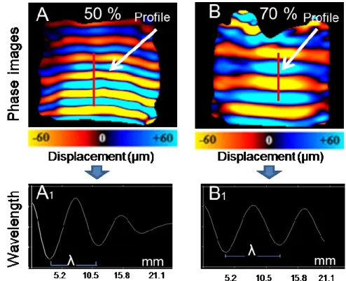
along the red profile, for the three frequencies (70, 90, 110 Hz). ... 108 Figure 3.1: A-B: phase images obtained from MRE tests performed on phantoms with different plastic concentrations. A1-B1: Behaviors of the waves traveling along the red profile. ... 113 Figure 3.2: A-B: Axial and sagittal anatomical images of the phantom (50%) where the fibers
and plastic sheet are localized. Phase images obtained through MRE experiments performed at 90Hz with the round driver in contact with the media without inclusion (A1-B1) and with inclusion (A2-B2). Red arrows indicate the direction of the wave propagation. ... 114 Figure 3.3: A-B-C: Views of the axial (A) and sagittal (B) anatomical images of the phantom
(50%) with inclusion and the muscle (C). A1-B1: Result of the MRE experiments
(90Hz) performed with the tube driver attached around the phantom. C1: MRE
tests (90Hz) performed on thigh muscle. Wave direction indicated by arrows along the red profile. ... 115 Figure 3.4:Viscoelasticparameters(G’,G”)measuredbyrheometer ... 116 Figure 3.5 : Behaviours of the wave obtained at 60, 80 and 100 Hz ... 117 Figure 3.6: Illustration of the three MRE steps to obtain the phase image. A (step #1): The
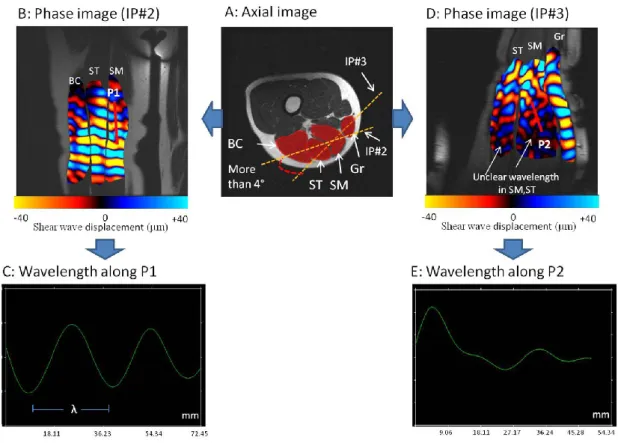
first column showed the orientation of the imaging plan (IP) as represented by a dashed line, within the target muscle. B (step #2): Sagittal images obtained from step #1 and represented the investigated muscles along the thigh. C (step #3): MRE sequence was performed on the selected sagittal image leading to the acquisition of the phase image, representing the displacement of the shear waves within the muscle. ... 119 Figure 3.7: Visualization of clear and unclear wave propagation. A: Axial image with two
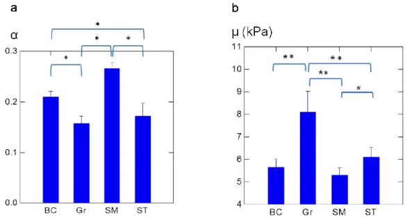
different orientations of the imaging planes (IP#2, IP#3) through semimembranosus (SM) and semitendinosus (ST). Phase images showing clear (B)wavewithmeasurablewavelength(λ)(C)andunclear(D)waveswithnon measurable wavelength (E). P1: Profile 1, P2: Profile 2. ... 121 Figure 3.8: Shear modulus (µ) with SEM obtained for the different thigh muscles and adipose
tissues. ... 122 Figure 3.9: Phase images of Gr muscle at different frequencies (70, 90, 110 Hz) ... 123 Figure 3.10: Representationofthewavelengths(λ)measuredwithinthegracilis(Gr)muscle,
along the red profile, for the three frequencies (70, 90, 110 Hz). ... 123 Figure 3.11: Mean±SEMofthedynamicexperimentalviscoelasticparameters(a:G’,b:G”
8
muscles. ... 124 Figure 3.12: Mean ± SEM of the viscoelastic parameters (a: viscosity(η).b:elasticity (µ1). c:
elasticity (µ2)) of the four thigh muscles (semimembranosus (SM),
semitendinosus (ST), biceps (BC), and gracilis (Gr) muscles) obtained from the Zener model. (**P < 0.05, *P < 0.1). ... 126
Figure 3.13: Comparison of the viscoelastic parameters (mean ± SEM ) (a: ratio b: elasticity µ).of the four thigh muscles (semimembranosus (SM), semitendinosus (ST), biceps (BC), and gracilis (Gr) muscles) obtained from the springpot model. (**P <0.05, *P <0.1). ... 127
9
Table 1-1:ListofconversionsbetweenLamecoefficients,Young’smodulus,Poisson’sratio,
and for an isotropic elastic homogeneous medium ... 34
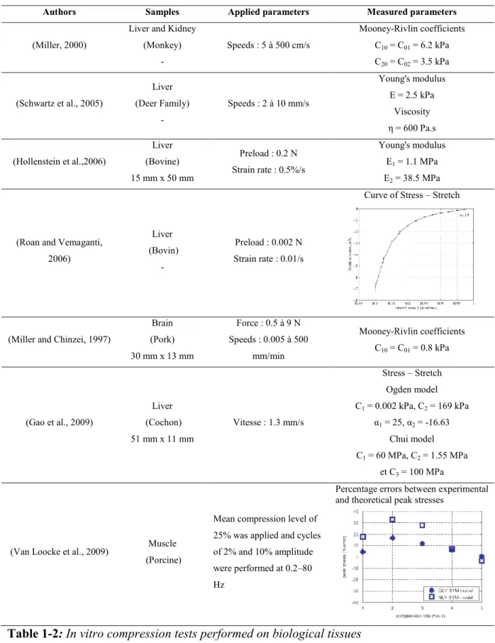
Table 1-2: In vitro compression tests performed on biological tissues ... 43
Table 1-3: Mean of the shear modulus (µ) of healthy muscles at rest and in contraction. Several muscles are mentioned such as biceps, flexor digitorum profundus (FDP), tibialis anterior (TA), medial gastrocnemius (MG), lateral gastrocnemius (LG), soleus (Sol), vastus lateralis (VL), vastus medialis (VM), Sartorius (Sr), and the quadricepsfemoris(QF).“⊥”denotes the stiffness measured perpendicular to the musclefibers,“‖”denotesstiffnessmeasuredparalleltothemusclefibers.MVC: maximum voluntary contraction. ... 63
Table 1-4: Mean of the shear modulus (µ) for pathological muscles at different condition. MVC: maximum voluntary contraction ... 64
Table 1-5: Viscoelastic properties of the phantoms using mechanical tests. ... 66
Table 1-6: Elastic properties of the phantoms ... 70
Table 3-1: Experimental viscoelastic data for the large phantom (50%) ... 117
Table 3-2: Summary of the viscoelastic parameters (G’, G”) measured with MMRE and HFUS technique at three drive frequencies (mean standard deviation). ... 118
Table 3-3: Rheological model parameters (mean SEM) and error of the fit measured from MMRE tests realized from four thigh muscles ... 125
10
GENERAL INTRODUCTION ... 15
CHAPTER 1
LITERATURE REVIEW ... 17
A. The skeletal muscle architecture ... 20
1. Introduction ... 20
2. Different types of muscle in the body ... 20
3. Chemical composition of muscle ... 21
4. Multi-scale Structure of skeletal muscle ... 21
4.1 Organization of the muscle fiber ... 21
4.2 The functional unit of muscle ... 24
4.3 The thigh muscles ... 25
4.3.1 Composition of the thigh muscles ... 25
4.3.2 Determination of the morphological properties with imaging techniques ... 26
4.3.3 Aponeurosis ... 28
B. Mechanical properties of the muscle ... 28
1. Functional characteristics of skeletal Muscle Tissue ... 28
2. The Hill model ... 28
3. Hooke's law ... 30
4. Stress and strain Tensors ... 31
5. Tensor of elasticity in isotropic medium ... 31
6. Incompressibe property ... 34
7. Propagation of waves in a soft material ... 35
8. Viscoelastic comportment ... 38
8.1 Elastic properties ... 38
8.2 Viscous properties ... 39
C. Techniques used for the characterization of the mechanical properties. ... 42
1. In vitro methods ... 42
1.1 Compression tests ... 42
1.2 Indentation tests ... 44
1.3 Dynamic Mechanical Analysis (DMA) ... 44
1.4 Torque meter technique ... 45
2. In vivo methods ... 45
11
2.3 Myotonometric ... 46
2.4 Elastography techniques ... 46
2.4.1 Introduction ... 46
2.4.2 Ultrasound (US) elastography techniques... 47
2.4.3 Magnetic resonance elastography (MRE) technique ... 52
I. Introduction ... 52
II. Description of the technique ... 53
2.4.4 Applications ... 60
D. Phantoms developed for elastography ... 65
1. Mechanical tests ... 66
2. Magnetic resonance elastography Tests ... 67
3. Mechanical properties ... 70
References ... 71
CHAPTER 2
MATERIELS AND METHODS ... 89
A. Phantom study ... 92
1. Phantom preparation ... 92
2. Development of phantom with similar muscle architecture ... 93
3. Development of a device to stretch the fiber ... 94
4. Determination of the mechanical properties ... 94
1. Hyper-Frequency Viscoelastic Spectroscopy (HFVS) ... 94
2. Magnetic Resonance Elastography tests ... 95
2.1 MR elastography set-up for the artificial muscle ... 95
2.2 Multifrequency MRE set-up performed on the homogeneous phantom... 96
2.3 Phase Image processing and data analysis ... 98
2.4 Summary of the different tests applied to the developed phantoms. ... 101
B. Thigh muscle study ... 102
1. Ethics Statement ... 102
2. Participants ... 102
3. Experimental configuration ... 102
4. Acquisition of the anatomical and phase images of the muscle ... 105
5. Phase Image Processing and Data Analysis ... 107
12
A. Phantom study ... 113
1. Elastic properties of the phantoms as a function of the: ... 113
1.1 Concentration of plastisol ... 113
1.2 Type of drivers ... 113
2. Viscoelastic properties of the phantoms: ... 116
2.1 Hyper-Frequency Viscoelastic Spectroscopy (HFVS) tests ... 116
2.2 Multifrequency MRE tests ... 117
B. Muscle thigh study ... 119
1. Propagation of the shear waves within the nine muscles ... 119
2. Comparison of the elastic property between the nine muscles at rest condition ... 121
3. Comparison of the viscoelastic property between the four muscles (ST, SM, BC, Gr) at rest condition using rheological model ... 122
CHAPTER 4
... 128
DISCUSSION AND PERSPECTIVES ... 128
A.
Phantom study ... 130
B.
Thigh muscle study ... 131
1. Elastic property ... 131
2. Viscoelastic property ... 133
CHAPTER 5
... 139
SUMMARIES ... 139
A.
Summary of the in vitro studies ... 140
B.
Summary of the in vivo studies ... 141
CHAPTER 6
... 142
RESUMES ... 142
A.
Résumé de l'étude in vitro ... 143
13
GENERAL
15
Muscle is a biological tissue whose mechanical properties vary with activity. Skeletal muscles are vital in the normal activities of a human being. Their main functions are to produce force and cause motion. The real-time estimation of muscle contractile properties is difficult due to the changes that may exist between muscle size, morphology and the exercised force. There are many muscular disorders which affect muscle function or structure, e.g. spastic paraplegia, muscular dystrophies or myositis. Our knowledge of muscle changes in diseases and treatments remains incomplete. Thus, the development of a non-invasive in vivo technique could provide information on a contracted or at rest muscle and will be essential to improve our understanding of muscle tissues. Biopsies and palpations remain the conventional clinical tests to diagnose and to monitor (Hsieh et al., 2000; Lew et al., 1997; Palacio-Torralba et al., 2015a) diseases, respectively. However, these techniques are invasive and subjective.
MRE (Magnetic Resonance Elastography) is a non-invasive medical imaging technique, developed with magnetic resonance imaging (MRI) (Bensamoun et al., 2007; Brauck et al., 2007; Debernard et al., 2011a, 2011b; Dresner et al., 2001), which allows assessment of the shear elasticity of tissues by applying a mechanical or compression excitation. Motion-sensitive MR sequences have been introduced to analyze the propagation of shear waves created by this excitation, through soft tissues (Muthupillai et al., 1995). MRE was applied to different healthy (Green et al., 2013a) and pathological soft tissues (Bensamoun et al., 2007, 2011a; Serai et al., 2012; Venkatesh et al., 2008) in order to provide quantitative data to the clinician from superficial to deep areas. This data would track the evolution of a disease, to better know the pathophysiology of this disease, to choose the most suitable treatment and to evaluate long-term effects of treatment with a gain of tissue function.
Recent application of MRE has studied skeletal muscle biomechanics (Bensamoun et al., 2006a; Debernard et al., 2011a). The aim of my thesis is to develop experimental protocols to characterize the mechanical properties of healthy thigh muscles with MRE technology (Magnetic Resonance Elastography). A better knowledge of muscle behavior, through analysis of its mechanical properties, will in improve the diagnosis, the treatment, and the follow-up of muscle disorders. Thus, a database of the muscle viscoelastic properties (G', G") have been constituted with the passive state of the thigh muscles.
16
structural properties to the investigated muscles. This test-objets will enable to test, MRE parameters, MRE sequence, and to develop new protocols before to apply in vivo the MRE muscle test. The particularity of the laboratory BioMechanic and Bioengineering (BMBI), where this PhD project belongs, is to associate experimental and numerical research. Thus, the present experimental functional properties will be used for the numerical model.
This manuscript is composed of four chapters.
The first one will be devoted to some anatomical reminders on the muscle tissue, followed by a state of the art of the experimental techniques used for the mechanical characterization of muscle (in vivo) and phantom (in vitro).
In the second chapter, the different materials and methods developed in this study will be explained through two parts:
The first in vitro part is devoted to the development and characterization of a test object, which has the same structural and mechanical properties as the muscle.
The second in vivo part aims at developing experimental MRE protocols to determine the viscoelastic properties of healthy thigh muscles.
The third chapter will present the results of these experimental in vitro and in vivo analyses.
The fourth chapter will provide a discussion of all the results, with the future experiments follow-up by the fifth chapter composed of a conclusion.
17
CHAPTER 1
LITERATURE
REVIEW
18
CHAPTER 1
LITERATURE REVIEW ... 17
A. The skeletal muscle architecture ... 20
1. Introduction ... 20
2. Different types of muscle in the body ... 20
3. Chemical composition of muscle ... 21
4. Multi-scale Structure of skeletal muscle ... 21
4.1 Organization of the muscle fiber ... 21
4.2 The functional unit of muscle ... 24
4.3 The thigh muscles ... 25
4.3.1 Composition of the thigh muscles ... 25
4.3.2 Determination of the morphological properties with imaging techniques ... 26
4.3.3 Aponeurosis ... 28
B. Mechanical properties of the muscle ... 28
1. Functional characteristics of skeletal Muscle Tissue ... 28
2. The Hill model ... 28
3. Hooke's law ... 30
4. Stress and strain Tensors ... 31
5. Tensor of elasticity in isotropic medium ... 31
6. Incompressibe property ... 34
7. Propagation of waves in a soft material ... 35
8. Viscoelastic comportment ... 38
8.1 Elastic properties ... 38
8.2 Viscous properties ... 39
C. Techniques used for the characterization of the mechanical properties. ... 42
1. In vitro methods ... 42
1.1 Compression tests ... 42
1.2 Indentation tests ... 44
1.3 Dynamic Mechanical Analysis (DMA) ... 44
1.4 Torque meter technique ... 45
2. In vivo methods ... 45
2.1 Palpation ... 45
19
2.3 Myotonometric ... 46
2.4 Elastography techniques ... 46
2.4.1 Introduction ... 46
2.4.2 Ultrasound (US) elastography techniques... 47
2.4.3 Magnetic resonance elastography (MRE) technique ... 52
I. Introduction ... 52
II. Description of the technique ... 53
2.4.4 Applications ... 60
D. Phantoms developed for elastography ... 65
1. Mechanical tests ... 66
2. Magnetic resonance elastography Tests ... 67
3. Mechanical properties ... 70
20
1.
A. The skeletal muscle architecture
1.
Introduction
Muscle tissues are a system capable of changing its length, exert force and convert chemical energy to mechanical energy. The tissues that generate movements of the human body are the striated or skeletal muscles. The body contains over 600 skeletal muscles representing 40-50% of the total weight of the human body (Bonnel et al., 2009). The contraction of skeletal muscle, placed under the control of the somatic nervous system, doesn’t only allows humans to move in its environment, to control, modify, seize and move objects but also, it plays an important role in body temperature regulation.
2.
Different types of muscle in the body
There are three types of muscles in the human body, namely the smooth muscle, the cardiac muscle, and the skeletal muscle (Figure 1.1).
- The skeletal muscle tissues:
Skeletal muscles form approximately 40 % of the body weight in men and 32 % of that in women (Sherwood, 2015). Their function is to engage and to mobilize the skeleton. They are the third key element of the locomotor system. This muscle is called "striated" because its macroscopic observation suggests parallel streaks with each other. Its activity is voluntary and is dependent on the somatic nervous system. Skeletal muscle is an essential component of the body and is primarily responsible for the production of the movement.
- The smooth muscle tissues:
They are found in the walls of the organs, vessels and bronchi. Their work is independent of their wills and therefore is under the control of the autonomic nervous system.
- The heart muscle tissues:
They are striated and their activity is involuntary, but under the control of the autonomic nervous system. Although there are significant differences in structures, mechanical properties and control mechanism between these three types of muscles.
21
Figure 1.1: Types of skeletal muscles
3.
Chemical composition of muscle
The skeletal muscle is constituted of about 75% water and 20% protein; the rest consists of inorganic salts and other substances such as high energy phosphate, urea, lactic acid and various minerals, enzymes and pigments, ions, amino acids, fats and sugars.
The most abundant muscle proteins are myosin, actin and tropomyosin. They represent respectively 52%, 23% and 15% of the muscle protein content. In addition, it is about 700 mg of myoglobin per 100 g of muscle tissue (Robertson, 1961)
4.
Multi-scale Structure of skeletal muscle
4.1 Organization of the muscle fiber
- Circular Muscles: These muscles appear circular in shape and are normally sphincter muscles which surround an opening such as the mouth and the eyes.
- Convergent Muscles: These are muscles where the origins (the attachment to a fixed bone, usually the proximal attachment) are wider than the point of insertion. This fiber arrangement allows a maximum force production.
- Parallel or Fusiform Muscles: Parallel muscles have fibers which run parallel to each other and are sometimes called strap muscles such as biceps femoris, semitendinosus, gracilis, biceps brachii and sartorius. They cause large movement because they are long muscles which are not very strong but have good endurance.
22
- Pennate Muscles: Muscles with fibers that run oblique to insert the tendon are called
pennate muscles. They can be divided into:
Unipennate muscles have their fibers arranged in a diagonal direction to insert onto the tendon that allow great strength such as vastus medialis and vastus lateralis,
Bipennate muscles have two rows of muscle fibers which are placed in opposite diagonal directions, allowing a high power but a less range of motion such as rectus femoris.
Multipennate: As the name suggests multipennate muscles have multiple rows of diagonal fibres with a central tendon that are inserted into two or more tendons.
The physiological cross-section (P.C.S), which is the area that cuts all the fiber of the muscle and often used to approximate the number of muscle fibers, is much larger in pennate muscles (Figure 1.2).
Figure 1.2:The three types of muscle-tendon arrangement, a) the parallel-fibered muscle, b) the unipennate muscle and c) the bipennate muscle. P.C.S. marks the physiological
23
These types of fiber differ in their morphology, their contractile and biochemical properties and play an important role on the developed force. Their distribution in the muscles varies from one muscle to another. Histology with coloring techniques (Brooke and Kaiser, 1970; Brooke MH and Kaiser KK, 1970; Choi and Kim, 2009) have distinguished three types of muscle fibers, divided into two major groups (figure 1.3), slow fibers (I) and fast fibers (II) (Pette and Vrbová, 1985)(Plaghki, 1985). They have each their own specificities.
Figure 1.3: Identification of slow and fast fibers, according to Kim and Choi, 2009
- Slow fibers (type I) : They have a high level of oxidative enzymes, low glycogen level and a high density of mitochondria. They contract slowly and have high resistance to fatigue. They are rich in myoglobin and blood capillaries that causes their red color.They are found in the muscles having a postural function.
- Fast fibers (type II) : On the contrary they are subdivided into two types of fibres, IIA (red) and IIB (white) which are able to contract quickly and have a lower resistance to fatigue.
Slow fibers are always solicited the first whereas the fast fibers are only solicited during important efforts and short periods.
The skeletal muscle architecture is the structural property of the whole muscles that dominates their function. The skeletal muscles are usually fixed on the bone at each of their ends via a tendon and there are several levels of organization in a skeletal muscle as shown in Figure 1.4 (Marieb and Hoehn, 2014).
The skeletal muscle is composed a large number of smaller bundles of muscle fascicles, which are separated by connective tissue such as epimysium, perimysium, endomysium and
24
sarcolemma. The muscle fascicle is composed of many skeletal muscle cells, it is known as muscle fiber, which has a cylindrical shaped cell measuring from 10 to 100 micrometers as diameter and until 75 cm as length (Sherwood, 2015). Each muscle fiber is protected by a cell membrane called the sarcolemma. The muscle fiber is composed of a set of myofibrils.
Figure 1.4: multi scale organization of the muscle system
Myofibrils have specific contractile intracellular elements that are composed of a succession of sarcomeres in series. The sarcomere is the smallest contractile intracellular element and consists of thin (actin) and thick (myosin) myofilaments that, through their interactions, can perform a shift that induce tension production in muscle, through interconnectivity and movement with each other (Huxley and Simmons, 1971)(Huxley and Taylor, 1958). Several proteins are presented in the muscle cell. Indeed, besides actin and myosin which are contractile proteins, it contains regulatory proteins such as troponin and tropomyosin or structural like titin, nebulin and alpha-actinin of the muscle system.
4.2 The functional unit of muscle
The principal function of skeletal muscle is to produce movement of the body set or body parts and perform work through coordinated and voluntary muscle contraction such as lifting weights or walking. Moreover, skeletal muscles are important for maintaining the position of the body and give it its shape. It also generates heat as a by-product of muscle activity, which assists in maintaining normal body temperature.
25
The fibers are surrounded by endomysium and include a set of myofibrils surrounded by a membrane called the sarcolemma. Typically there are hundreds of these membranes in one cross section of a muscle fiber. It is divided into segments called sarcomeres.
Sarcomeres are composed of thick filaments (composed of a protein, myosin, whose diameter is 12 to 18 nm) and thin filaments (compound of another contractile protein, actin, which has a diameter of 5 to 8 nm). They are surrounded by two dark colored bands (characterizing anisotropic zones, highly birefringent) called Z-discs or Z-lines. These Z-discs are dense protein discs that do not allow easily the passage of light and thus appear black under the microscope.
The area between the Z-discs is fourthly divided into two lighter colored bands of actin at either end called the I-bands (characterize isotropic zones) and a darker, grayish band of myosin in the middle called the A-band .
During muscle contraction, each muscle sarcomere shortens as the thin filaments slide closer to each other between the thick filaments so that the Z lines are pulled closer (Figure 1.5).
Figure 1.5: Sarcomere structure
4.3 The thigh muscles
4.3.1 Composition of the thigh muscles
The thigh is composed of ten muscles located in the anterior, medial and posterior area. - The anterior thigh muscles: The muscles of the anterior part of the thigh include the
quadriceps group and Sartorius. The quadriceps muscle is a group of four muscles that originate in different locations and that form the front of the thigh. Rectus femoris forms the middle portion of the quadriceps, vastus lateralis is the lateral-most of the
26
quadriceps, vastus medialis is the most medial of the quadriceps and vastus intermedius lies behind the rectus femoris. The main action of this muscle group is the extension and the stabilization of the leg.
Figure 1.6: Axial image with the investigated thigh muscles. Quadriceps muscle (VL: vastus lateralis, VI: vastus intermedius, VM: vastus medialis, RF: rectus femoris), Sr: sartorius, Gr: gracilis, AD: adductor, hamstring muscles (ST: semitendinosus, SM: semimembranosus, BC:
long and short biceps)
- The medial thigh muscles: The muscles of the medial part of the thigh have the adductor and gracilis muscles that bring the thigh toward the midline and that rotate it. - The posterior thigh muscles: The posterior thigh is known as the hamstring muscles.
They are composed of three muscles, semimembranosus, semitendinosus and biceps, that form the back of thigh. Theirs roles are to flex the leg.
4.3.2 Determination of the morphological properties with imaging techniques
The ultrasonic imaging (US), is one of medical imaging technique that is widely used in clinical studies, has been used to make an evaluation of muscle geometric parameters. In the muscle, the muscle fibers are arranged in different orientations compared to aponeurosis. The angle formed between these muscle fibers, which connect the tendon and aponeurosis, is
27
called the pennation angle (figure 1.7). Ultrasound is simplest method to visualize the orientation of the muscle fascicles. Moreover, any authors use this technique to evaluate the muscle thickness, the pennation angle (θ) (figure 1.7) , and the fascicle length (Abe et al., 1998, 2000; Arampatzis et al., 2007; Brechue and Abe, 2014; Chow et al., 2000; Fukunaga et al., 1992, 1997a, 1997b; Hodges et al., 2003; Ichinose et al., 1997; Reeves and Narici, 2003).
Figure 1.7: Schematic representation of muscle architecture.
These studies are valuable because they have defined a new typology of the human body muscles according to the arrangement of the muscle fibers.
Several studies use the ultrasound imagery technique to determine the structural parameters of muscle such as: the muscular thickness (Kubo et al., 2003), the thickness of the subcutaneous adipose tissue (Heckmatt et al., 1988a; Saito et al., 2003; Scholten et al., 2003), the pennation angle (Debernard et al., 2011a; Fukunaga et al., 1997a; Henriksson-Larsen et al., 1992; Hodges et al., 2003; Kawakami et al., 1993; Kubo et al., 2003; Maurits et al., 2004), the length of fascicule (Kubo et al., 2003), and the muscle area (Cross-Sectional Area (CSA)) (Maurits et al., 2004; Walton et al., 1997).
These studies were capable of determining the healthy muscle architecture (Heckmatt et al., 1988a; Maurits et al., 2004; Scholten et al., 2003) in order to study the effects of hypertrophy (Kawakami et al., 1993), the age, the sex (Kubo et al., 2003; Men et al., 1985; Young et al., 1984) and neuromuscular diseases (Heckmatt et al., 1988b; Maurits et al., 2004; Scholten et al., 2003) on the eventual modification of the muscular architecture.
These parameters along with the muscular area (Beneke et al., 1991) and the muscular volume (Walton et al., 1997) can be defined with magnetic resonance imaging (MRI) to
28
decrease the acquisition protocol, the methods and cutting numbers by optimizing the acquisition time for these purposes (Fukunaga et al., 2001; Lund et al., 2002; Morse et al., 2007; Nordez et al., 2009; Tracy et al., 2003). However MRI has certain limitation of visualization and characterization of the depth of the muscular architecture compared to the ultrasonic imaging technique (US).
4.3.3 Aponeurosis
A white or yellowish membrane is glossy, very resistant and is made of intersecting fibers, either termination or intersection muscles that attach the bone or muscle envelope to hold it in place. It constitutes a very thin envelope that surrounds and connects the various organs of our body. This tissue is found deep in the muscles, bones, nerves, heart, lung, cortex, ligaments and internal organs. Around the muscles and muscle bundles, the aponeurotic bulkheads form groups called lodges that allow easily to differentiate each muscle (Figure 1.7)
B. Mechanical properties of the muscle
1. Functional characteristics of skeletal Muscle Tissue
The Muscle is the only body tissue with the properties of irritability, contractility, extensibility and elasticity.
The irritability property of a muscle is the ability to respond to a stimulus, that produces a muscle contraction. Stimulus can be internal or external. The Contractility refers to the ability to shorten or contract causing an increase in the tension between its ends and length that may shorten, or remain the same. The extensibility means the ability to stretch in response to a force and the elasticity is the ability to recoil when a stretch force is removed to returns the muscle to its resting length.
The characterization of the skeletal muscles properties are carried out by complex mechanical behaviours such as anisotropy, quasi-incompressibility, non-linear elasticity and viscoelasticity with time dependent creep and stress relaxation, rate dependence and hysteresis in addition to the ability to undergo large deformation (Fung and Cowin, 1994).
2. The Hill model
For further explanation and to identify the behavior of the muscle in its active and passive states, simple models have been proposed with the combination of springs and
29
daspots elements. The first model, that represents muscle response, is a simple spring. It characterizes the effect of the muscle length as a function of the developed force. To study the influence of the speed of contraction, a viscous element is added in parallel by Hill (Hill, 1922). In 1927, Levin and Wyman complicated the Hill model by adding an elastic component in series to take into account the influence of the tendon on the myo-tendon complex (Levin and Wyman, 1927). This model was modified by Hill in 1938 and revisited by Shorten in 1987. It is a three-component model; where each component reflects a property of the muscle behavior (Goubel and Lensel-Corbeil, 2003):
Figure 1.8: Mechanical model of muscle Shorten-Hill (1987); CC: Contractile component, PEC: Parallel elastic component, SEC: Series elastic component
- Contractile component (CC) (muscle fiber) is similar to a shock absorber and has their shortening velocity related to the force developed by the muscle.
- Parallel elastic component (PEC) (muscle membrane or fascia) represents the muscle behavior when reaching important extensions.
- Series elastic component (SEC) (tendon) explains the significant and rapid decrease of efforts when the muscle is contracted at a constant length (isometric conditions) and subjected to a rapid shortening. It also intervenes in enhancing the muscle performance by storing mechanical potential energy developed by the muscle.
Specific tests performed on in vitro muscle and then extended to in vivo tests allow the studying of each of these components: Contractile component (CC), Elastic component parallel (ECP) and Elastic component series (ECS).
30
The elastic component series and the contractile component allow the modeling of the specific behavior within the myofibril, the muscle contraction. The parallel elastic components allow the reproduction of the elastic comportment of the conjunctive tissue that includes the muscle membranes: endomysium, perimysium and epimysium.
The continuum mechanics is the field of physics interested in the deformation of the solid and the fluid flow and that describes all mechanical changes of an environment: static compression or extension and the mechanical wave propagation of all kinds. To discuss continuous mechanics, several hypotheses must be respected: a continuous medium, homogeneity and isotropy. Mechanical waves are the carriers of information in the continuum mechanics that allow us to identify the mechanical properties of tissues. These waves will be propagate through tissue with parameters dependant on its properties.
The theory of the continuous medium mechanics is based on the law made by Hooke (Chapman, 2004). This law allows to connect the force exerted on a solid to its deformation. It also describes all the mechanical modification of the object on the environment: static compression or extension and the propagation of the mechanical waves of all kinds. Subsequently, it is possible to introduce parameters that can describe the continuous media.
3. Hooke's law
Muscle tissues are non-linear, viscoelastic, anisotropic and incompressible. However, to simplify the analysis, the mechanical properties are usually modeled to behave the muscle as linear, elastic and isotropic materials (Bensamoun et al., 2006a; Krouskop et al., 1998; Ophir et al., 1999). The elasticity is the quality of a material to be deformable while resuming its original shape when the applied stress disappears. The conventional theory of elasticity describes the mechanical properties of elastic solids where stress is proportional to strain in small deformations. Thus, the elasticity of a muscle means that the muscle can return to its original length and form after a contraction or a stretch.
Robert Hooke created a law named hook’s law proving that strength is always proportional to the elongation. Originally developed to describe the behavior of the springs, this law is then applied by physicists in soft solid element in the case of small deformations. When a deformation (strain) is applied to the solid, volume internal forces to the object will be created in order to reduce the solid to its equilibrium state. These volume internal forces are called contraints (stress).
31
Hooke’s law allows to connect a stress (σ) (force) to a strain (ε) (local elongation) and elasticity (E):
4. Stress and strain Tensors
They allow to extend the concepts of strain and stress to a case of an elementary volume of three dimension according to the tensor formalism. They are defined as follows (Figure 1.9):
The stress tensor corresponds to the ith component of the stress applied to the facet normal (vector).
The strain tensors are defined as
, where u is the field displacement.
Figure 1.9: Different simplest cases of stresses and strains and their associated tensors (illustrated in 2D) .
5. Tensor of elasticity in isotropic medium
Hooke's law can be extended to a three-dimensional problem when considering an elementary volume, in the approximation of small strains that links the stress tensor ( ) to the strain tensor ( ) with an elastic tensor. In fully anisotropic homogeneous material, the stress-strain relationship can be described by Hooke’s law:
where is the stress matrix and the strain matrix and is a fourth order tensor that
32
is sometimes named the elastic rigidity tensor and contains 81 elements that completely
describe the elastic characteristics of the medium. Because of the symmetry of and , only 36 elements of are independent in general cases. The stiffness tensor consists of 21 independent variables due to symmetry considerations (i.e. ).
By exploiting the symmetries of the medium, the tensors of stresses ) and the strains ( ) can be reduced to tensors each having only 6 items. Moreover, only 2 independent constants of rigidity are present in for linear homogeneous isotropic purely elastic medium: Lame
coefficients λ and μ have a stress dimension; λ is related to longitudinal strain and μ to shear strain. However, the transversely isotropic material contains only six independent parameters due to the axis of symmetry.
11 12 13 12 11 13 13 13 33 44 44 66 0 0 0 0 0 0 0 0 0 0 0 0 0 0 0 0 0 0 0 0 0 0 0 0 C C C C C C C C C C C C
Lame coefficients are defined from as follows:
C11 = C22 = C33 = λ+2µ
C12 = C13 = C23 =λ
C44 = C55 = C66 = (C11 - C12)/2 = µ
The strain–stress relationship can be written as:
33
Employing the lame coefficient, it is possible to define a couple of equivalent parameters (Storaa et al., 2003) whose physical signification differs slightly. This allows to choose the most suitable couple (torque) to the problem:
K = λ + 2/3µ
where K is the compression module (bulk modulus) and µ is the shear modulus.
The coefficient K is then called the compression module since it connects the compression strain to the strain. This compression module characterizes the change in volume of the solid when stress is applied simultaneously on all sides and perpendicular to all the points of the surface which surround the solid (principle of hydrostatic pressure).
The second coefficient lame µ corresponds to the shear modulus which connects the shear strains to stresses. This shear modulus reflects the difficulty to twist (shear) the solid. Although this coefficient is small in soft biological tissues, it is not negligible. This module changes a lot with tissue pathology, which makes it interesting medically to characterize this parameter. In the literature, the shear modulus (μ) is defined as "shear modulus" when it is independent of the frequency and as "shear stiffness" at a given frequency (Bensamoun et al., 2007; Debernard et al., 2011b; Dresner et al., 2001).
However, it is possible to study the mechanical properties of a solid following a different approach. Under homogeneous deformations, such as hydrostatic pressure, the stress tensor is constant throughout the solid.
Young's modulus (E) and Poisson's ratio (ν) are two parameters that characterize the solid. They are defined as:
ν = λ/2(λ+µ) and E = µ (3λ+2µ)/ (λ+ µ)
Poisson's ratio (ν) defines the relationship between uniaxial crushing and resulting lateral elongation and is 0.5 for incompressible solids. Young's modulus (E) is the potential crush, always uniaxially, a solid having the ability to deform laterally. Since the stresses are applied uniaxially (in a single direction), other parameters are free to deform. It is possible to express the two lame coefficients (λ) depending on the Young's modulus E and Poisson's ratio ν:
34
The table below lists the conversions between Lame coefficients, Young’s modulus, Poisson’s ratio, and for an isotropic elastic homogeneous medium.
E ν λ μ C11 C12 C44 Table 1-1: ListofconversionsbetweenLamecoefficients,Young’smodulus,Poisson’sratio, and for an isotropic elastic homogeneous medium
6. Incompressibe property
Muscle is an incompressible material. The volume of the muscle remains constant for any given transformation during compression (Figure 1.10). Due to the conservation of the volume, strain in a certain direction has to be compensated by an inverse strain in other directions. The sum of the strain in all directions must be null (Støylen, 2001) under the hypothesis of no shear strain. An incompressible material is also called an isochoric material.
Figure 1.10: The principle of incompressibility. The volume of the incompressible object remains constant during (Lindberg, 2013).
35
This mechanical property is due to the important quantity of water in the muscle. It is usually used as a Poisson coefficient modeling. Poisson’s ratio () is a material constant that can be used to characterize the deformation in such material. This constant describes the relation between the transversal and the axial strain and varies between -1 and 0.5. Even though there are very little quantitative data on the Poisson’s ratio of soft biological tissues, researches in animal, human and phantom studies have shown that the Poisson’s ratio of soft tissues and mescle is close to 0.5 (Fung and Cowin, 1994; Krouskop et al., 1998; Ophir et al., 1999; Støylen, 2001).
The finite element models (Blemker et al., 2005; JOHANSSON et al., 2000; Leclerc et al., 2013a; Martins et al., 1998; Oomens et al., 2003; Yucesoy et al., 2002) use incompressible or nearly incompressible materials to represent the passive muscle behavior.
Muscle tissues are composed mainly of water and are nearly incompressible, the compression module K is very large compared to the shear modulus µ. The compression modulus K of these tissues is of an order of several GPa contrary to shear modulus μ which is of an order of some tens of kPa.
For medical applications, Poisson's ratio is close to 0.5, K >> µ and K ≈ λ. Therefore, the Young's modulus E can be simplified to:
E = 3µ
7. Propagation of waves in a soft material
The study of the shear wave propagation in the soft tissue is a very important issue to determine the mechanical properties. The elastography technique, which determines the mechanical properties, is based on this wave propagation which will be described subsequently.
In the case of an elastic solid and supposing that the deformations are low, it is possible to express the equation of motion in function of the mechanical properties of the solid and the displacement (u):
E
grad
u
E u t u 1 2 2 1 1 2 2 236
In the case of a plane elastic wave traveling along the x direction, the equation of motion becomes: 2 2 2 2 2 2 2 2 1 0 1 0 x x l y y t u u x V t u u x V t
where Vl is the velocity of the longitudinal waves (or compression waves, seismic waves P)
and Vt is the velocity of the transversal waves (or shear waves, seismic waves S) (Figure
1.11).
These velocities (Vl and Vt) can be expressed in function of the Young’s modulus (E) and
Poisson's ratio (ν):
1 2 1 1 2 2 1 3 l t E K V E E V As a function of the direction of propagation of the wave, two types of waves can be distinguished:
1. The compression waves (longitudinal) VL, where the wave propagation direction is
parallel to the displacement (Figure 1.11a).
2. The shear waves (transversal) VT, where the wave propagation direction is
37
Figure 1.11: Representation of the compression (A) waves and the shear (B) waves.
The expressions of longitudinal and transversal velocities in function of the compression and shear moduli show that the propagation of longitudinal waves is governed by the compression module while the propagation of transverse waves is governed by the shear modulus, which is connected to the Young's modulus.
In homogeneous isotropic elastic medium, it is possible to split the acoustic waves in independent longitudinal and transverse waves, each travelling at a speed VL and VT
respectively.
For quasi incompressible and soft biological tissues, the compression wave propagation velocities are 1500 m/s, similar to water, and the shear wave propagation velocities are between 1 m/s and 20 m/s. Thus, shear wave could be measured and the soft tissues have different shear moduli (Robert, 2009) (Figure 1.12).
38
Figure 1.12: Variation of the mechanical compression and shear modulus of various
biological tissues. Ranges associated with each modulus for a given tissue type are indicated
by the shaded regions (Sarvazyan et al., 1998).
8. Viscoelastic comportment
The word viscoelastic is composed of the words "viscous" and "elastic"; thus a viscoelastic material exhibits both viscous (fluid) and elastic (solid) behaviors, such as the muscle tissue.
Skeletal muscle tissue, like many other biological tissues, is a viscous material. The viscosity has a direct effect on the mechanical properties of the passive muscle. Best et al., (1994) realized a test of traction on rabbit muscle at strain rate between 0.01s-1 and 2 s-1 and showed that the response of the stress is dependent on the strain rate. Similarly Myers et al (1995, 1998) conduct the same type of experiment but with higher strain rate: 1 s-1, 10 s-1 and 25 s-1. For the same strain at 20%, they get a Young's modulus of 1.75 MPa for 1 s-1, and 2.79 MPa for 25 s-1, showing a significant increase in the stiffness as a function of the strain rate.
8.1 Elastic properties
The strain–stress relationship is valid when the strain is instantaneously
provoked by stress, i.e., no dephasing process occurs. The equations of the compression and the shear waves can be reformulated according to the two longitudinally (ul) and transversely
39 2 2 2 2 2 2 2 2 t u x u t u K x u t t l l
These equations assume that the waves, that propagate in the medium, remain unchanged and can propagate to infinity if the considered solid doesn’t exceeded by limit. However shear waves attenuate rapidly during their propagation in biological tissue. In order to take this attenuation in the wave equation, it is necessary to consider that the shear modulus is not a real number but a complex number. It is possible to approach the problem solely in terms of shear considering only the complex shear modulus (G*) and Hooke's law where the wave equation becomes: u G t u G * 2 2 *
The behavior of the material is then mainly described by the expression of the complex shear modulus. The complex shear modulus can simplify the notations and its expression allows modeling of behavior solids. The different behavior modes correspond to the rheological models whose complexity varies according to the desired use.
8.2 Viscous properties
The behavior of viscoelastic materials under uniaxial loading may be represented by means of conceptual models composed of elastic and viscous elements, which provide physical view point and have didactic value. One can build up a model of linear viscoelasticity by considering the combinations of the linear elastic spring and the linear viscous dash-pot. These are known as rheological models or mechanical models.
The complex shear modulus (G*) and its mechanical behavior is characterized with different rheological models whose complexity varies according to the desired usage. The study of the characteristics of deformable bodies (elasticity, viscosity, plasticity, fluidity) is better known as the rheology study. Indeed the objective of the rheology is to study the fluid flow and the viscoelastical properties of the deformable solid. The two basic components used in rheology are the spring and the dash-pot.
40
The rheological models can be characterized with respect to their static and dynamic behavior.
The static characterization is obtained through two types of experiments: creep and relaxation: - Creep consists in applying a constant stress to the system and observes its time deformation.
- Relaxation consists in eliminating comes to release the system stress and observe its behavior at the equilibrium.
The dynamic characterization consists in expressing the shear modulus in function of to the characteristics of the rheological model in consideration and characterizes the mechanical behavior in function of on the applied frequency.
Figure 1.13: Rheological models used in the literature for the characterization of biological tissues.G*isthecomplexshearmodulus,μisshearmodulus,ηisviscosity,fisthefrequency
andωisthepulsation(2.π.f)
The Maxwell model can be represented by a purely viscous dash-pot and a purely elastic spring connected in series. This model is particularly adapted for modeling liquid deformations.
Jeffrey model contains one spring and two dampers and is used normally in fluids,
The Kelvin–Voigt model also called the Voigt model, is a viscoelastic material that has both
the elasticity (µ) and the viscosity (η) properties and can be represented by a purely viscous dash-pot and purely elastic spring connected in parallel. The behavior of these objects, described by a Voigt model, is closer to the behavior of a solid rather than that of a liquid.
41
The Zener model also known as the standard linear solid (SLS) model is a method that models the behavior of a viscoelastic material using a linear combination of springs and dash-pot to represent elastic and viscous components respectively. This model consists of two elasticity coefficients μ1 and μ2. Often, the more similar Maxwell model and the Kelvin– Voigt model are used. These models are often proven insufficient since the Maxwell model does not describe creep or recovery and the Kelvin–Voigt model does not describe stress relaxation. SLS is the simplest model that predicts both phenomena.
The springpot model is condensed between the spring and dash-pot. The viscoelastic behavior of biological tissues cannot be modeled perfectly with different models previously introduced. The springpot (µ, model take three parameters into account. The parameter represented a weighting factor between a purely elastic behavior ( = 0) and a purely viscous behavior ( = 1). For the springpot model, (µ) and ( were linearly dependent, meaning that either the value of (µ) or (were fixed.
42
C. Techniques used for the characterization of the mechanical
properties.
In this part, the experimental techniques are performed in vitro and in vivo in order to determine the mechanical properties of soft biological tissues.
1.
In vitro methods
1.1 Compression tests
In a compression test, the sample is maintained between two plates (steel) while the normal force (F) is measured as a function compression (h), performed at an imposed speed after preloading (Figures 1.14). Then from the slope of the force-displacement curve, the Young's modulus can be calculated as
Δh ΔF A h h Δh A ΔF ε σ E 0 0 0 0
where is the uniaxial compressive stress, is the longitudinal strain, ΔF is the difference of the compressive forces, A0 is the initial section of the sample and Δh is the height
difference between the initial state h0 and the compressed state.
Figure 1.14: a: Custom built for the characterization of mechanical properties of liver (Schwartz et al., 2005). b: Experimental setup high speed cyclic testing rig. (A) Top platen; (B) bottom platen; (C) LVDT transducer; (D) static load cell; (E) dynamic load cell; and (F)
43
The characterization of mechanical properties of several tissues using the compression tests are summarized in this table:
Authors Samples Applied parameters Measured parameters
(Miller, 2000)
Liver and Kidney (Monkey) - Speeds : 5 à 500 cm/s Mooney-Rivlin coefficients C10 = C01 = 6.2 kPa C20 = C02 = 3.5 kPa (Schwartz et al., 2005) Liver (Deer Family) - Speeds : 2 à 10 mm/s Young's modulus E = 2.5 kPa Viscosity η = 600 Pa.s (Hollenstein et al.,2006) Liver (Bovine) 15 mm x 50 mm Preload : 0.2 N Strain rate : 0.5%/s Young's modulus E1 = 1.1 MPa E2 = 38.5 MPa
(Roan and Vemaganti, 2006) Liver (Bovin) - Preload : 0.002 N Strain rate : 0.01/s
Curve of Stress – Stretch
(Miller and Chinzei, 1997)
Brain (Pork) 30 mm x 13 mm Force : 0.5 à 9 N Speeds : 0.005 à 500 mm/min Mooney-Rivlin coefficients C10 = C01 = 0.8 kPa (Gao et al., 2009) Liver (Cochon) 51 mm x 11 mm Vitesse : 1.3 mm/s Stress – Stretch Ogden model C1 = 0.002 kPa, C2 = 169 kPa α1 = 25, α2 = -16.63 Chui model C1 = 60 MPa, C2 = 1.55 MPa et C3 = 100 MPa
(Van Loocke et al., 2009) Muscle (Porcine)
Mean compression level of 25% was applied and cycles of 2% and 10% amplitude were performed at 0.2–80 Hz
Percentage errors between experimental and theoretical peak stresses