Social Security in Belgium: Distributive Outcomes

IZA DP No. 1486

Social Security in Belgium:

Distributive Outcomes

Alain Jousten

Mathieu Lefèbvre

Sergio Perelman

Pierre Pestieau

Social Security in Belgium:

Distributive Outcomes

Alain Jousten

Université de Liège, CEPR and IZA Bonn

Mathieu Lefèbvre

Sergio Perelman

Pierre Pestieau

Discussion Paper No. 1486

February 2005

Any opinions expressed here are those of the author(s) and not those of the institute. Research disseminated by IZA may include views on policy, but the institute itself takes no institutional policy positions.

The Institute for the Study of Labor (IZA) in Bonn is a local and virtual international research center and a place of communication between science, politics and business. IZA is an independent nonprofit company supported by Deutsche Post World Net. The center is associated with the University of Bonn and offers a stimulating research environment through its research networks, research support, and visitors and doctoral programs. IZA engages in (i) original and internationally competitive research in all fields of labor economics, (ii) development of policy concepts, and (iii) dissemination of research results and concepts to the interested public.

IZA Discussion Papers often represent preliminary work and are circulated to encourage discussion. Citation of such a paper should account for its provisional character. A revised version may be available directly from the author.

IZA Discussion Paper No. 1486 February 2005

ABSTRACT

Social Security in Belgium: Distributive Outcomes

The paper analyzes the link between old-age income programs and economic outcomes in Belgium. We use a simulation methodology to construct an average pension generosity variable. Our regression analysis explores the link with distributional outcomes in income, consumption and more subjective indicators. Results document the weak link between average generosity and distributional outcomes across a heterogeneous population.

JEL Classification: H31, H55, I31, I32

Keywords: pensions, inequality, social security, elderly

Corresponding author: Alain Jousten

Université de Liège Département d’Economie 4000 Liège / Sart Tilman Belgien

Email: ajousten@ulg.ac.be

∗ _{Financial support from FRFC (2.4544.01) is gratefully acknowledged. The paper was written while}

1. Introduction

Even though the Belgian social security system initially belonged to the contributory Bismarckian tradition, it progressively became more and more redistributive. Today, replacement ratios are much higher for low-income earners than for workers with higher than average earnings, and internal rates of return vary a great deal across people. Pestieau and Stijns (1998) present Eurostat data from 1991 illustrating the net replacement rates of one- and two-earner couples, ranging from as high as 91 per cent for a single-worker household earning two thirds of average wages to 53 per cent for an upper middle-class two-earner couple earning twice average earnings. These observations are confirmed by OECD data from 1997 and 1999 for below-average earners showing replacement rates broadly in line with those of the previous authors. The increased degree of redistribution resulting from the social protection programs is the result of a series of factors. First, the social assistance program has seen its generosity increase over the years with strong increases both in levels and above-inflation indexation of benefits. Second, the social insurance programs have generated an increasing role for minimum benefit provisions. For example, minimum benefits have over the years become much more favorable for people with long careers but low earnings levels. Third, the main social insurance program, namely the one applicable to the wage-earners of the private sector, is characterized by a proportional contribution on all wages, whereas only those up to pensionable earnings enter the benefit formula, which accounts for a large part of the inherent redistribution of the system. Last, but not least, early retirement provisions have introduced yet another dimension to the redistributive nature of the systems, with strong redistribution occurring towards people retiring early from the labor force. In other words, the emphasis of the Belgian social system seems to have shifted from an insurance objective based on the Bismarckian example towards yet another tool of income redistribution. In a certain sense, social security is nowadays at least equally concerned with averting absolute and most of all relative poverty in old age by providing all workers with a sufficient income level, a fact mirrored by the strongly income-dependent replacement ratios.

Against this backdrop, reforms that endanger the redistributive function of social security are hard to sell to increasingly conservative social partners. The word conservative has to be read and understood in its original sense, meaning a desire to preserve the current structures, rather than in the nowadays more common sense to describe political parties on the right of the political divide. Employers and employees have grown used to the advantages of massive early retirement with costs shifted to an all too willing government, as has again been illustrated in early 2005 by the "temporary" extension of early retirement provisions at age 56 for two more years for private sector workers.

The objective of the present paper is to explore the effects of social security benefits on the well-being of elderly. Previous studies focused on two datasets, the Panel Survey of Belgian Households (PSBH) and an administrative dataset stemming from the tax administration. Delhausse and Perelman (1998) and Perelman et al. (1998) found evidence that poverty is no less prominent among the elderly than among the young, a finding that is totally consistent with the increased social spending and the explicitly redistributive nature of the Belgian social insurance system (see table 1). The indicators of poverty these authors use are the "poverty rate" - as defined to be the fraction of families with less than 50 percent of standardized median income - as well as the inter-quartile ratio of standardized income between the top and the first income quartiles. The main weakness of these indicators is that they exclusively focus on

2 income concepts, and thus only give a very partial view on people's well-being. Indeed, while income data might be easier to obtain, other parameters such as consumption levels as well as measures of subjective well-being might also be of interest. The present paper attempts to shed some light on these measures in the Belgian context by extending the range of indicators well-beyond pure income-based indicators.

Table 1: Poverty, inequality and age

Poverty Rate Interquartile ratio

Age

PSBH (1994) All 4,7 3,31

60-70 6,2 3,60

70-80 4,4 3,17

80 + 5,5 3,07

Fiscal data (1995) All 5,6

45-60 4,0

60+ 3,8

Source: PSBH: Delhausse and Perelman (1998); Fiscal data: Perelman et al. (1998)

In our regression analysis, we attempt to isolate the pure effects of the social insurance system's benefit generosity from other determinants of well-being such as wage income. To attain this objective, we focus our attention on people aged 65 and above. Below that age, wage income still represents the major income source for a non-negligible fraction of the population. The link between social insurance programs and the degree of well-being of the population is not an easy question. All things being equal we would expect that a generous social security system – generous in terms of average replacement ratio – generates more redistribution, less poverty than a less generous system. But things cannot be kept equal and one can show that for political economy reasons a contributory system is more likely to be more generous than a redistributive

system.1

The remainder of the paper is organized as follows. Section 2 reviews the key features of the Belgian social security system. The following sections then describe the data we use for our analyses and the analysis thereof, before the final concluding section.

1 _{Pestieau, P. (2003), Social security and the well-being of the elderly. Three concepts of generosity,}

3

2.

Basic features of the Belgian social security system

The Belgian social security system has three major components, one for public employees, one for the self-employed and one for private sector employees. These are supplemented by a welfare scheme providing a minimum old age pension to individuals not entitled to any of the first three; this latter scheme is means tested.

We start our brief overview of the institutional setting with the system covering private sector employees, the system that represents the majority of workers and pensioners in Belgium. Social security is financed by tax-deductible employer and employee contributions and government general revenue on a pay-as-you-go basis. Social security benefits are indexed to the cost of living and on an occasional and purely discretionary basis to the growth rate of the economy. The normal retirement age of the system is 65, with a transitory regime applicable to women until the year 2009. The normal retirement is progressively being shifted upwards to 65 as a result of European Union requirements of equal treatment of the sexes and reaches age 63 in 2005. De facto, this increase implies an important reduction of benefits for women as full-career requirements as well as the averaging period becomes longer and hence more difficult to attain. The more relevant situation for our analysis is however the one in place prior to July 1997 as most of the data at hand stem from that period.

Benefits depend on the length of the work career (full benefits require 45 years, except for the transitory regime for women), on the marital status and on income, the latter being indexed to the present using cost-of-living adjustments, mostly based on price-indexation. There are ceilings and floors, applicable both to pensionable earnings and pensions. For example, a worker with yearly income of 33 000 € in 2003 (about the average) is entitled to a replacement ratio of 49% if married and 39% if single, granted that he is 65 years old and has a full career of

45 years. (For a woman, in 2004, the normal retirement age is 63)2.

Within the current pension system, retirement is possible as early as at 60 and continued work is possible after age 65 with the explicit consent of the employer. For example, a worker with the same income but being 60 years of age and having a 40-years-long career would be entitled to a replacement ratio of 46% if married and of 36% if single.

This adjustment is simply due to the fact that the career is incomplete with a loss of pension rights equal the 5/45. Before 1997 the adjustment for such an early retirement within the window 60-65 was more important. For each year of early retirement there was a penalty of 5% of benefits. Before the age of 60, private sector employees can leave the labor force and get benefits. The standard exit routes are unemployment insurance and early retirement schemes, as well as to a lesser degree disability insurance. In Belgium, before 55, unemployment is the most popular way of retiring and after that age unemployment remains a possibility but there are also all kinds of early retirement schemes. The prominent role of unemployment insurance in the Belgian retirement landscape is a result of a special regime for old-age unemployed. In the past, it sufficed to be aged more than 50 to benefit from this preferential system which effectively gave this category of unemployed the privilege of a waiver from the requirement to search for a new job as well as the requirement to periodically report to the administration to maintain the status. The regime underwent some changes in the early years of the new millenium, with

4 access to the full waivers being more restrictive and henceforth limited to people aged 58 and more. In previous work, Dellis et al (2004) have shown that these public programs (combined with the imagination of companies' human resource departments) explain early retirement quite well.

Public sector pensions are on average much higher than those of private sector employees. They are taken out of the general federal revenue. Civil servants solely pay contributions at a rate of 7.5% to cover survivors' benefits. In contrast to the private sector, retirement is mandatory at the latest at age 65 for both men and women. However, there exists a variety of ways of retiring earlier than at this age. First, retirement through disability insurance is possible. Opting for an incomplete career is also possible. Finally, there are special regimes for example for teachers, army and police employees. Here again, benefits are linked to income earned with ceilings and floors. Civil servants' benefits are continuously indexed not only to the cost of living, but also to productivity increases. However, it has to be said that the increasingly decentralized structure of the Belgian state has not been without consequences for the public sector pensions. With the transfer of competences to economic regions (Flanders, Wallonia and Brussels) and language communities (Dutch, French and German), wage bargaining has increasingly become decentralized. As a result, pay regimes and indexation rules have multiplied to a point where it is hard to keep track of the wide variety of regimes applicable.

The self-employed retirement scheme is the newest and the least generous of the three. Furthermore, the normal retirement age for the self-employed workers is 65, again with a transitory regime for women. Earlier retirement is possible as of age 60, though much harder and linked to rather severe career requirements. Early retirement is also much less advantageous than in the other systems as benefits are not only adjusted through an incomplete career mechanism that is similar to the wage-earner scheme, but they are also adjusted downwards by 5 per cent per year of anticipation. Further, the self-employed are not eligible for any of the other common pathways into retirement, namely unemployment insurance or special early retirement schemes as these do simply not exist for this particular subgroup of the population.

Table 2: Data availab

ility of measures of w

ell-being

Antwerp and University

of Liège) 1992 → 20 02 60 → 85 Household in co m e poverty rate (40% of m edian incom e) - OECD Consum ption 60 → 85 87 Total / food household consum ption - OECD Household C onsum ption Surve y (National institute of statistics) 1979 , 19 88, 1995, 1996 , 19 97, 1999, 2000 (7 waves) Total / food h ousehold consum ption povert y rate ( 40% of median consum ption) - OECD 270

Percent of people ver

y satisfied Self-ass ess ed life satisfaction Eurobarom et er 1975 → 20 01 (y early ) 60-64 ( 65) 65-69 ( 70), 70-74 ( 75), 75-79 ( 80), 80-84 ( 85), (cohort average) 229

Percent of people fairl

y or

not

very

satisfied

Self-reported health status

Eurobarom eter 1987 , 19 89, 1990, 1993 , 20 01 60-64 ( 65) 65-69 ( 70), 70-74 ( 75), 75-79 ( 80), 80-84 ( 85), (cohort average) 25

Percent of people in ver

y o

r

fairly

good

3.

Outcome data

For the needs of our analysis of outcomes in terms of well-being, we use data from various

sources that enclose both objective and subjective indicators.3 _{To get the best possible picture of}

the effects that the generosity of the retirement income systems might have on outcomes, we

focus our attention on the people between the ages of 65 and 85.4 _{Table 2 summarizes the data}

sources, as well as the availability of the data over time.

We distinguish a series of indicators of average well-being in a given year: income, consumption, happiness, health and the indicators of poverty. The interested reader find a series of plots describing the evolution of selected indicators of well-being over time in appendix A. By definition, these are indicators of average well-being across the entire population, and hence do not necessarily account for the wide variability within the population. Further, it has to be stressed that these are purely annual measures, which means that they do not take any life-cycle considerations into account. The latter remark is of a particular importance when thinking about the self-employed where the distinction between current and life-cycle income is likely to be the largest.

Consumption data are drawn from the household budget survey (HBS) of the National Statistics office (INS). We have data from seven different waves at our disposal spanning the period from the late seventies to the year 2000. On the basis of this data, we compute three dependent variables: average consumption, relative poverty and absolute poverty. The data are grouped in two different ways. The first way of proceeding is to group people into pure age-cells. This way of proceeding is useful when regressing the INS data on observed benefit levels as such data are only available along a pure age-breakdown. The second way of proceeding, which is our preferred approach, is to group people into cells defined by education levels as well as by age. In this latter approach, the use of 5-year brackets instead of yearly groups helps us avoid insufficient cell-size. Our preference for the second approach resides in the fact that education levels help us to get a much more detailed picture of the differences among the Belgian population than a pure age indicator ever could do.

The income data originates form the HBS (late 1970's and 1980's) as well as the Panel Survey of Belgian Households (PSBH) for later periods ranging from 1992 till 2001. Income data used in what follows has to be understood as after-tax income. For the same reasons as mentioned for the consumption data, we use two different groupings according to which independent variable we use in the regressions of outcomes in terms of well-being on system generosity indicators. Households are the units of observation in both the HBS and the PSBH. Therefore, all our analysis will be based on the household as the relevant economic unit. When computing average consumption and income levels, we apply OECD household equivalence scales to derive a measure of average disposable income in the household.

We classify households into two categories, those with people aged 65 and more in the household that we call elderly households and those that have no household member aged 65 or above that we call non-elderly.

When computing the household average income for all households with people aged 65 or

3 _{All EUR concepts in the present paper are expressed in 2001 EUR.} 4 _{No reliable data available above age 85.}

7 more, we take the mean over the entire sample, weighting each household/family by the number of persons in the relevant age range. To compute household mean income for those 65 and more, we take a weighted mean income over all households, where the weight is the number of persons aged 65 and more in the household. So any household in which an elder resides gets some weight and weights increase with the number of elders living there, de facto person-weighting the data.

On the other hand, for measures of income and consumption for non-elderly households, we exclude any household containing an elderly person. This way, the numbers derives for non-elderly households is a pure measure of resources of the non-non-elderly, uncontaminated by potential spillovers resulting from the presence of elderly in the household. Once again, we should weight the averages computed for groups of non-elderly by the number of persons in the household to get a person-weighted measure.

Using this categorization into elderly and non-elderly households, we proceed to the definition of different measures of well-being, both absolute and relative:

- Total household income/consumption

- Absolute income/consumption poverty: share of elderly in households with income/consumption below a fixed threshold. The threshold is 40% of median non-elderly income/consumption in earliest year of data, updated across time by the consumer price index to account for inflation.

- Relative income/consumption poverty: share of elderly in households with incomes below 40% of the median income of non-elderly households.

The two other data sources are more subjective as they summarize the perceived health and happiness reported by individuals. Health data originate from the Eurobarometer survey, a cross-national survey carried out over a wide range of European countries. Given its rather general nature and the relatively restricted sample size in the age-group of interest to us, we regroup the data on health status found in the surveys of 1987, 1989, 1990, 1993 and 2001 into

one binary indicator of health and group people into five-year age-cells.5

A priori, happiness is clearly the least objective but potentially the most accurate measure of well-being, as it captures not only the material situation an individual is in, but also the perception of the individual about his situation. As such, it is not found in the classical household surveys, with the only exception being the Eurobarometer survey. We use the life-satisfaction question from this source to construct two indicators of happiness: the proportion of people that are very happy, and those that are very unhappy or not very happy. Surprisingly, happiness information is available for a wider time span than health information starting as early as 1973.

5 _{People responding that they are in very good or fairly good health standing are classified as "in good}

Table 3: Data availab

ility on benefits

Measure Source

Years

available

Ages available

Num

ber of

observations

Variable

description

Actual benefits

Statis

tiqu

e

annuelle des

bénéficiaires de

presta

tion

s

(National Office of

Pensions)

1970

→

2001

60

→

85

832 average

benefit

Earning prof

ile

Adm

inistrative

CGER database

Age of withdrawal

from

the labour

force

Labour Force

Survey and

Statis

tics alm

anach

(Nationa

l In

stitu

te

of

statis

tic

s)

1970

→

2001

50-54 ,

55-60,

60-64,

65+

32 Labor

force

participa

tion

rate

Weighting rate of

schem

es

Bouillot and

Perelm

an (1995)

1970

→

2001 50

→

65

Num

ber of people

involved in each

schem

3.

Benefit data

In line with the objective of the paper, we now define measures of benefit generosity that will serve as explanatory variables in the regression analysis of the next section.

Benefit generosity is not a straightforward measure to use, as observed measures of generosity as measured in administrative data is not necessarily a valid data source. The reason for this skepticism with respect to actual data on generosity is that the data itself is already the result of a retirement decision, that in turn is again at least partly influenced by indicators of well-being we observe as a dependent variable on the left-hand side of our regression analysis.

We thus proceed by a simulation methodology, whereby we use data from various sources to construct benefit indicators that are less problematic. The data sources at hand are listed in table 3. Simulated pension benefits are the result of a weighted aggregation for a representative worker aged between 50 and 85 years over the period 1970 to 2002. We assume that his professional career was either as a wage earner, a civil servant or a self-employed with the

corresponding weights. Due to a severe lack of data for individuals belonging to the

self-employed and the civil-servant systems, we focus on wage-earners in our discussion of

simulation methodology. 6

For the representative male we assume that he has a full career, which means that he paid social security contributions and accumulated the corresponding pension rights at each age, starting at age 20. For the representative female, the situation is slightly more complex. In the context of the wage-earner scheme, we consider three different situations to account for the wide variability in labor force participation rates for females: a full career scenario, an incomplete career pathway and a third case where we assume that the woman was never attached to the labor force. We compute the proportion of women belonging to each of these categories on the

basis of labor force participation rates by age and cohorts.An incomplete career means that the

representative person was at work, paid social security contributions and collected pension

rights, for some years, and out of work for the rest of time. 7

When a married woman had an incomplete career or was never attached to the labor force, we have to go one step further in our computation of benefits. Under the rules of the wage-earner, the self-employed and the means-tested pension schemes, husbands are entitled to a supplementary amount (equivalent to 25% of their pension) if their spouse has no earnings or is

not beneficiary of social replacement allowances, including other social security pensions.8 _This

de facto means that married women with incomplete career abandon their own pension rights in favor of the supplementary spousal allowance, as their own pension rights are often smaller than this supplement.

6 _{We approximated the civil servant system by analogy with the wage-earner system. For self-employed,}

we had to rely in average date further limiting the information content of the data. For example, we cannot distinguish careers of men and women by lack of sufficient data for these two systems.

7 _{For reasons of data tractability, we assume that the partial working career corresponds to a woman}

having positive, but lower earnings during the entire career rather than full earnings for part of the career.

8 _{We do not consider the mean-tested, public pension scheme called GRAPA in our simulations of}

pension benefits given that the representative individual was entitled in all the analyzed situations to receive pension benefits higher than the guaranteed minimum.

10 The proportion of men and women in each pension scheme (wage-earners, civil servants and self-employed) by year and age cohort, was estimated using social security administrative sources. Given to the lack of available data, we do not consider mixed careers in these schemes. That means that our representative individual is assumed to belong to only one scheme over his entire professional life in contrast to the real world situation where mixed careers are not uncommon.

Moreover we consider alternative pathways into retirement. On the one hand, we compute pension benefits for the three mentioned schemes taking into account early retirement provisions within these systems. On the other hand, we also simulate the alternative unemployment (from 50 to 65 years old) and other early retirement (from 58 to 64 years old) routes that are available to wage-earners outside of the official retirement system. Within each scheme average pension benefits for men and women at each age (50 to 85) and year are then aggregated using the observed path weights. Aged workers leaving the labor force prior to the earliest age at which they become eligible for benefits within any given pathway are assumed to receive benefits of zero euro. The weighting of the different pathways into retirement is based on the labor force participation rates in each year by the method of Latulippe as explained by

Scherer.9 _{People younger than 58 leave through the unemployment insurance system, those aged}

58 and 59 through early retirement, those between the ages of 60 and 64 through a mix of early retirement and retirement regimes, and those aged 65 exclusively through regular retirement programs. For any given year, benefits of people aged more than 65 are computed on the basis of those of people aged 65 to which we apply an adjustment factor based on data from National Pension Office (ONP-RVP).

To complete and enhance the information content of our benefit data, we do not restrict our attention to the baseline situation of one hypothetical synthetical individual of the entire population. We rather explore the data by separating people into education subgroups and income deciles within these education groups. We group people into then income and three education groups (those with primary, secondary and undergraduate degrees). We thus determine one synthetic earnings profile for each education/income subgroup, which leads us to a total of 30 profiles. Similarly, we compute profile-specific outcomes for these various profiles. The computation of the benefits for all people aged between 50 and 85 between the years 1970 and 2002 relies on the baseline income pattern that is shifted up and down for the 30 subgroups to adjust for their relative income position. The data are price-indexed to take prices inflation into account and finally averaged over the 9 firts income deciles to finally produce the 3 benefit profiles that we use for most of our analysis.

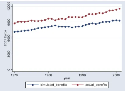
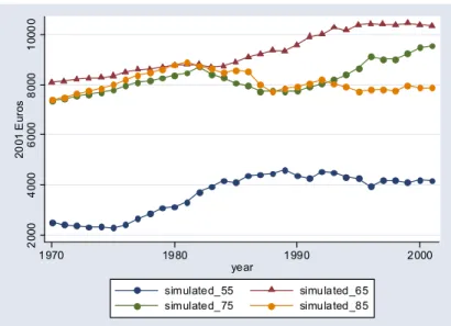
As it appears on Figures A-E of Appendix B, the profile of benefits over time is rather flat both on average and for specific years. Unsurprisingly, the profiles of observed and simulated benefits do not differ a great deal. Data on observed benefit levels are drawn from ONP-RVP files. We focus our attention on people who receive pensions exclusively from the wage-earner system between the ages of 60 (earliest retirement age) and 85 for the time-span ranging from 1970 to 2001. Mixed careers are excluded and no distinction can be made according to education group, as no administrative dataset in Belgium records education levels. To our surprise, figure E reveals that expected benefits have not always been increasing in age. Further,

11 benefits at age 85 have been declining at times, indicating that incomplete price indexation might be an issue in the Belgian context.

4. Regression

analysis

Table 4.1 and 4.2 summarize the key results of a series of regressions trying to explain a number of consumption- and income-related welfare indicators by the simulated benefits available. The data are separated into year, age and education level cells. For the purposes of the empirical

analysis, we restrict our attention to individuals aged 65 and more.10

Consumption exhibits strongly significant coefficients for the first two models (table4.1). The use of education dummies renders parameters insignificant. The same observations qualitatively hold true for relative poverty with a much less significant coefficient than consumption for the first two. The absolute poverty regression does not seem to lead to significant parameters in either specification.

Table 4.1 Consumption regression (years 1979, 1988, 1996, 1997, 1999 and 2000)

Dependent variable Model Simulated benefit

Coeff. t-value Number of _obs. R-Square

Consumption Linear 1.959 11.57 69 0.825

Age, Year dummies 2.016 11.96 69 0.847 Age, year, edu dummies -0.153 -0.42 69 0.921 Relative Consumption Poverty Linear -0.680 -1.94 69 0.212

Age, Year dummies -0.822 -2.45 69 0.361 Age, year, edu dummies 1.011 1.25 69 0.602 Absolute Consumption Poverty Linear -0.235 -0.91 69 0.395

Age, Year dummies -0.360 -1.52 69 0.554 Age, year, edu dummies 1.102 1.81 69 0.681

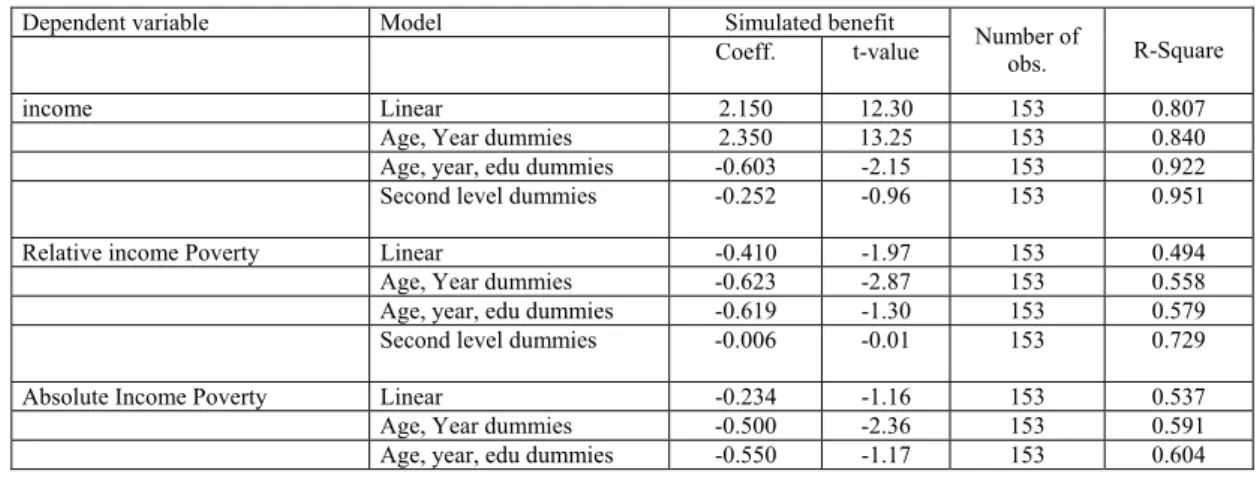
Table 4. 2 Income regression (years 1979, 1988, 1992 to 2002)

Dependent variable Model Simulated benefit

Coeff. t-value Number of _obs. R-Square

income Linear 2.150 12.30 153 0.807

Age, Year dummies 2.350 13.25 153 0.840 Age, year, edu dummies -0.603 -2.15 153 0.922 Second level dummies -0.252 -0.96 153 0.951 Relative income Poverty Linear -0.410 -1.97 153 0.494

Age, Year dummies -0.623 -2.87 153 0.558 Age, year, edu dummies -0.619 -1.30 153 0.579 Second level dummies -0.006 -0.01 153 0.729 Absolute Income Poverty Linear -0.234 -1.16 153 0.537

Age, Year dummies -0.500 -2.36 153 0.591 Age, year, edu dummies -0.550 -1.17 153 0.604

10 _{For the interested reader we attach regressions with a cut-off age of 60 instead of 65 in Appendix C.}

12 Second level dummies 0.123 0.30 153 0.796

Table 4.2 contains the results of the income regressions. Because of the significantly larger number of observations, we perform one additional regression that does not only account for age and year dummies, but also second level dummies capturing the interaction of age and year on the one hand with the education dummy on the other. The use of education dummies in the regressions leads to non-significant parameters on the benefit variable, except for the income regression. In line with the findings for consumption, we mostly find significant coefficients when considering simple models with linear age trends or pure age dummies.

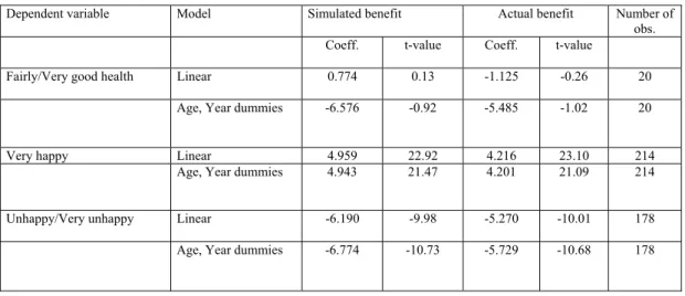
The health data used in table 4.3 are grouped by year and age (5-years basis). As we do not have any information on education level for these observations, we limit our attention to the simple linear and dummy regression where the benefit variable represents the average of benefits available to people of different education levels. The life satisfaction data of table 4.3 are constructed the same way. We present results for both actual and simulated benefits. The table shows that life satisfaction seems to be strongly affected by actual and simulated benefits, while health does not seem to follow the same pattern. The result of an insignificant impact of benefits on health should however be read with some prudence. One the one hand, the extremely small sample size clearly limits the degree of significance of the parameter estimates. On the other hand, a casual look at graph 7 of Appendix A documenting a free fall of self-reported health status over the years should caution the reader about the quality of the Eurobarometer data on health.

Table 4.3 Satisfaction and health regression (years 1987, 1989, 1990, 1993 and 2001 for health and

1973, 1975 to 2001 for satisfaction)

Dependent variable Model Simulated benefit Actual benefit Number of obs.

Coeff. t-value Coeff. t-value

Fairly/Very good health Linear 0.774 0.13 -1.125 -0.26 20 Age, Year dummies -6.576 -0.92 -5.485 -1.02 20

Very happy Linear 4.959 22.92 4.216 23.10 214 Age, Year dummies 4.943 21.47 4.201 21.09 214

Unhappy/Very unhappy Linear -6.190 -9.98 -5.270 -10.01 178 Age, Year dummies -6.774 -10.73 -5.729 -10.68 178

We proceed with the analysis of the link between benefits and well-being using actual benefits in tables 5.1 and 5.2. These regressions are not directly comparable to the preceding ones and are thus presented in separate tables. The key difference lies in the fact that individuals' education level is not observable in the ONP-RVP dataset that serves as a basis for our regressions.

13 We continue to define age cells as five-year age groups for reasons of insufficiency of data for the income regressions, in line with the approach applied to simulated benefits. For consumption on the other hand, we now have sufficient data to break age-cells down to a yearly basis and this way increase the richness of the data.

Table 5.1 Consumption regression with actual benefits (years 1979, 1988, 1996, 1997, 1999 and 2000)

Dependent variable Model Actual benefit

Coeff. t-value

Number of obs.

R-Square

Consumption Linear -0.121 -0.71 141 0.733

Age, Year dummies 1.670 8.73 141 0.647 Relative Consumption poverty Linear 0.694 1.76 141 0.160

Age, Year dummies -0.984 -2.71 141 0.223 Absolute Consumption poverty Linear 0.511 1.72 141 0.361

Age, Year dummies -1.105 -3.89 141 0.347

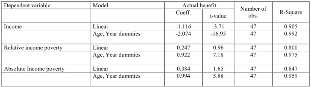
Table 5.2 Income regression with actual benefits (years 1979, 1988, 1992 to 2002)

Dependent variable Model Actual benefit

Coeff. _t-value Number of _obs. R-Square

Income Linear -1.116 -3.71 47 0.905

Age, Year dummies -2.074 -16.95 47 0.992 Relative income poverty Linear 0.247 0.96 47 0.800

Age, Year dummies 0.922 7.18 47 0.975 Absolute Income poverty Linear 0.384 1.65 47 0.847

Age, Year dummies 0.994 5.88 47 0.959

The results we obtain are puzzling at best. Actual benefits only seem to have a significant decreasing effect on poverty when we use the dummy regression. In all other cases, signs we observe on the poverty coefficients tend to show the contrary, namely increased poverty as a result of increased benefits. Our main interpretation of these effects is that actual benefits have a negative impact on consumption poverty because the benefit measure is simply not the accurate one. Absolute poverty is most likely affected by benefits received by the poor, while relative poverty is also affected by the benefits received by the richest decile of the population. Using a single benefit measure for actual benefits corresponds to the use of an average benefit measure for the population, thus benefit levels that are closest to those of the middle classes and not of the extremes of the income distribution.

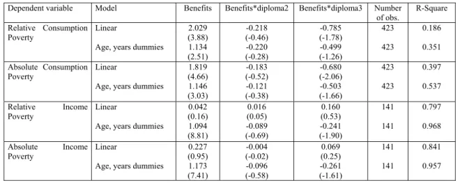
This intuition for the surprising results is reinforced when performing another set of regressions. We now use simulated benefits by education group for the poverty regressions, but no longer measure poverty by age-group and education but simply by age. The regression

Poverty = age + year + diploma2 + diploma3 + Benefits + Benefits*diploma2 + Benefits*diploma3 We obtain the results of table 6 indicating that overall poverty indicators worsen when simulated benefits for the least educated increase. Simulated benefits correspond to a complete working career, meaning that we simply do not accurately capture the effect of benefits on the

14 poorest people in the overall population. Hence, our benefit measures are most valid when working with relatively homogenous cells. Tables 4.1 and 4.2 are therefore an indication that benefits have the potential to decrease poverty within more homogenous cells.

Table 6 Poverty, benefits and education

Dependent variable Model Benefits Benefits*diploma2 Benefits*diploma3 Number of obs.

R-Square Relative Consumption

Poverty Linear

Age, years dummies

2.029 (3.88) 1.134 (2.51) -0.218 (-0.46) -0.220 (-0.28) -0.785 (-1.78) -0.499 (-1.26) 423 423 0.186 0.351 Absolute Consumption Poverty Linear

Age, years dummies

1.819 (4.66) 1.146 (3.03) -0.183 (-0.52) -0.121 (-0.38) -0.680 (-2.06) -0.503 (-1.66) 423 423 0.397 0.537 Relative Income Poverty Linear

Age, years dummies

0.042 (0.16) 1.094 (8.81) 0.016 (0.05) -0.089 (-0.69) 0.160 (0.53) -0.241 (-1.90) 141 141 0.797 0.968 Absolute Income Poverty Linear

Age, years dummies

0.227 (0.95) 1.173 (7.41) -0.004 (-0.02) -0.096 (-0.58) 0.069 (0.25) -0.261 (-1.61) 141 141 0.841 0.957

5. Conclusion

The purpose of this paper was to see how the social insurance retirement provisions affect the well-being of Belgian retirees. The results are hard to interpret and to some degree disappointing. They should however not be overvalued: given the crudeness of our benefit measure, particularly for the self-employed, it should not be surprising that the results are not more convincing.

The poor quality of our indicators of well-being can be the explanation, but not the only one. It is not sure that with better data, with the ideal data, one would get good results. We expect that generous social security benefits have a positive effect on the average well-being of retirees and, all things being equal on poverty in old age. But things are not equal and further the relation is not instantaneous; it is likely to be based on some lifetime perception. Further, it is not sure whether our indicators of generosity are really the ones we need within the context of a study of the welfare effect of the retirement system. Our indicators of average generosity do not necessarily give a truthful picture of generosity to those most touched by the consequences of poverty, namely low income wage-earners and self-employed.

15

References

Bouillot, L. et Perelman, S. (1995), Evaluation patrimoniale des droits à la pension en

Belgique, Revue Belge de Sécurité Sociale 37(4) :803-31

Delhausse, B. et S. Perelman (1998), Inégalité et pauvreté : mesures et déterminants, in

Commission 4, 13ème Congrès des Economistes Belges de Langue Française, CIFOP,

Charleroi.

Delhausse, B., S. Perelman et P. Pestieau, (2000), Le noyau dur de la pauvreté, in P.

Pestieau and B. Jurion (éds.), Finances Publiques, Finances Privées, Presses de l’ULG,

Liège.

Dellis, A., R. Desmet, A. Jousten and S. Perelman, (2004), Micro-modelling of

retirement in Belgium, in J. Gruber and D. Wise, Social Security Programs and

Retirement around the World. Microestimation, NBER, University of Chicago Press.

Mercer (2003), European Pensions Overview-Belgium, July 2003 www.mercerHR.com

Perelman, S., A. Schleiper et M. Stevart (1998), Dix années plus tard, d’un congrès à

l’autre : l’apport des statistiques …scales à l’étude de la distribution des revenus, in

Commission 4, 13ième Congrès des Economistes Belges de Langue Française, CIFOP,

Charleroi.

Pestieau, P., (2004), "Social security and the welfare of the elderly. Three concepts of

generosity", unpublished.

Pestieau, P. and J-Ph. Stijns (1999), “Social Security and retirement in Belgium”, in

Gruber, J. and D. Wise (1999), Social Security and retirement around the world, NBER

and Chicago University Press, Chicago, 37-71.

Appendix

Appendix A

Index value 100 is equal to 7158 for young and

6897 for elderly (2001 constant euros)

Graph 1 : Average income

0 50 10 0 15 0 19 79= 10 0 1979 1988 1997 2001 annee elderly young

index value 100 is equal to 2.06 for young and

2.79 for elderly

17 0 50 10 0 15 0 19 79= 10 0 1979 1988 1997 2001 annee elderly young

index value 100 is equal to 2.06 for young and

2.79 for elderly

Graph 3 : Income absolute poverty

10 0 12 0 14 0 16 0 18 0 197 9= 1 0 0 1980 1985 1990 1995 2000 year elderly young

Index value 100 is equal to 9960 euros for young and

7993 for elderly (2001 constant euros)

18 20 40 60 80 10 0 12 0 197 9= 1 0 0 1980 1985 1990 1995 2000 year elderly young

Index value 100 is equal to 3.09 for young and

6.39 for elderly

Graph 5 : Consumption relative poverty

0 20 40 60 80 10 0 197 9= 1 0 0 1980 1985 1990 1995 2000 year elderly young

Index value 100 is equal to 3.09 for young and

6.39 for elderly

19 0 20 40 60 80 10 0 197 3= 1 0 0 1973 1980 1990 2001 year elderly young

Index value 100 is equal to 45.14 for young and

46.60 for elderly

Graph 7 : Happiness – Very Happy

10 0 20 0 30 0 40 0 50 0 60 0 197 3= 1 0 0 1973 1980 1990 2001 year elderly young

Index value 100 is equal to 7.69 for young and

6.31 for elderly

20 85 90 95 10 0 19 87= 10 0 1987 1992 1997 2001 year young elderly

index value 100 is equal to 96.95 for young and

93.82 for elderly

21

Appendix B

Figure A : Actual and simulated benefits by year

0 30 00 60 00 90 00 1 200 0 20 01 E ur os 1970 1980 1990 2000 year primary secondary high_school

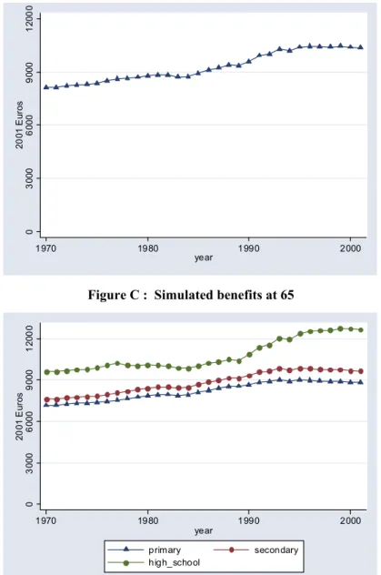
22 0 3 000 6 000 90 00 1 200 0 20 01 E ur os 1970 1980 1990 2000 year

Figure C : Simulated benefits at 65

0 3 000 60 00 9 000 1 200 0 20 01 E ur os 1970 1980 1990 2000 year primary secondary high_school

23 20 00 4 000 60 00 8 000 1 000 0 20 01 E ur os 1970 1980 1990 2000 year simulated_55 simulated_65 simulated_75 simulated_85

24

Appendix C

Table C1 Consumption regression (years 1979, 1988, 1996, 1997, 1999 and 2000)

Dependent variable Model Simulated benefit

Coeff. t-value Number of _obs. R-Square

Consommation Linear 1.488 9.84 87 0.756

Age, Year dummies 1.712 11.02 87 0.800 Age, year, edu dummies -0.345 -1.32 87 0.919 Relative Consumption Poverty Linear -0.579 -2.33 87 0.245

Age, Year dummies -0.703 -2.80 87 0.407 Age, year, edu dummies 0.131 0.24 87 0.613 Absolute Consumption Poverty Linear -0.284 -1.51 87 0.433

Age, Year dummies -0.330 -1.81 87 0.588 Age, year, edu dummies 0.359 0.86 87 0.692

Table C2 Income regression (years 1979, 1988, 1992 to 2002)

Dependent variable Model Simulated benefit

Coeff. t-value Number of _obs. R-Square

income Linear 1.270 9.35 192 0.726

Age, Year dummies 1.862 12.50 192 0.797 Age, year, edu dummies -0.279 -2.06 192 0.941 Second level dummies -0.267 -2.16 192 0.963 Relative income Poverty Linear -0.422 -3.09 192 0.423

Age, Year dummies -0.397 -2.39 192 0.475 Age, year, edu dummies 0.435 1.76 192 0.585 Second level dummies 0.708 3.37 192 0.774 Absolute Income Poverty Linear -0.225 -1.77 192 0.529

Age, Year dummies -0.348 -2.25 192 0.571 Age, year, edu dummies 0.033 0.14 192 0.611 Second level dummies 0.195 1.03 192 0.826

25

Table C3 Satisfaction and health regression (years 1987, 1989, 1990, 1993 and 2001 for health and

1973, 1975 to 2001 for satisfaction)

Dependent variable Model Simulated benefit Actual benefit Number of obs.

Coeff. t-value Coeff. t-value

Fairly/Very good health Linear -0.199 0.05 -2.819 -0.95 25 Age, Year dummies -5.87 -0.93 -4.827 -1.47 25 Very happy Linear 5.038 27.04 4.242 27.44 270

Age, Year dummies 5.040 25.81 4.233 26.07 270

Unhappy/Very unhappy Linear -6.830 -12.76 -5.759 -12.89 229 Age, Year dummies -7.355 -13.78 -6.181 -13.89 229

Table C4 Consumption regression with actual benefits (years 1979, 1988, 1996, 1997, 1999 and 2000)

Dependent variable Model Actual benefit

Coeff. t-value

Number of

obs. R-Square

Consumption Linear 0.047 0.40 176 0.742

Age, Year dummies 1.187 7.17 176 0.585 Relative Consumption poverty Linear 0.161 0.60 176 0.170

Age, Year dummies -0.789 -2.81 176 0.221 Absolute Consumption poverty Linear 0.001 0.00 176 0.377

Age, Year dummies -0.931 -4.12 176 0.329

Table C5 Income regression with actual benefits (years 1979, 1988, 1992 to 2002)

Dependent variable Model Actual benefit

Coeff. _t-value Number of _obs. R-Square

Income Linear -0.654 -2.60 59 0.914

Age, Year dummies -1.789 -14.37 59 0.989 Relative income poverty Linear 0.742 2.72 59 0.622

Age, Year dummies 1.373 8.01 59 0.926 Absolute Income poverty Linear 0.489 2.42 59 0.819

26

Table C6 Poverty, benefits and education

Dependent variable Model Benefits Benefits*diploma2 Benefits*diploma3 Number of obs.

R-Square Relative Consumption

Poverty

Linear

Age, years dummies

0.238 (0.91) 0.380 (1.62) -0.011 (-0.03) -0.044 (-0.16) 0.035 (0.12) -0.199 (-0.82) 528 528 0.176 0.383 Absolute Consumption Poverty Linear

Age, years dummies

0.160 (0.80) 0.328 (1.85) -0.002 (-0.01) -0.044 (-0.21) 0.052 (0.24) -0.193 (-1.05) 528 528 0.382 0.559 Relative Income Poverty Linear

Age, years dummies

-0.336 (-2.99) -0.365 (-3.90) 0.026 (0.18) 0.025 (0.20) 0.050 (0.34) 0.025 (0.19) 176 176 0.618 0.728 Absolute Income Poverty Linear

Age, years dummies

0.039 (0.18) 0.985 (6.69) 0.015 (0.06) -0.079 (-0.50) 0.177 (0.67) -0.211 (-1.35) 176 176 0.821 0.942