Numerical study of an optical regenerator exploiting self-phase modulation and spectral offset filtering at 40 Gbit/s

HAL Id: hal-00429627

https://hal.archives-ouvertes.fr/hal-00429627

Submitted on 16 Apr 2010

HAL is a multi-disciplinary open access archive for the deposit and dissemination of sci-entific research documents, whether they are pub-lished or not. The documents may come from teaching and research institutions in France or abroad, or from public or private research centers.

L’archive ouverte pluridisciplinaire HAL, est destinée au dépôt et à la diffusion de documents scientifiques de niveau recherche, publiés ou non, émanant des établissements d’enseignement et de recherche français ou étrangers, des laboratoires publics ou privés.

Numerical study of an optical regenerator exploiting

self-phase modulation and spectral offset filtering at 40

Gbit/s

Christophe Finot, Thanh Nam Nguyen, Thierry Chartier, Julien Fatome,

Stephane Pitois, Laurent Bramerie, Mathilde Gay, Jean-Claude Simon

To cite this version:

Christophe Finot, Thanh Nam Nguyen, Thierry Chartier, Julien Fatome, Stephane Pitois, et al.. Numerical study of an optical regenerator exploiting self-phase modulation and spectral offset filtering at 40 Gbit/s. Optics Communications, Elsevier, 2008, 281 (8), pp.2252-2264. �10.1016/j.optcom.2007.12.010�. �hal-00429627�

Numerical study of an optical regenerator

exploiting self-phase modulation

and spectral offset filtering at 40 Gbit/s

C. Finot

1

, T.N. Nguyen

2

, J. Fatome

1

, T. Chartier

2

,

S. Pitois

1

, L. Bramerie

2

, M. Gay

2

, J.-C. Simon

2

1

Institut Carnot de Bourgogne (ICB), Dept. OMR,

UMR CNRS 5209 Université de Bourgogne, 21078 Dijon, FRANCE christophe.finot@u-bourgogne.fr

2

FOTON (UMR CNRS 6082), ENSSAT,

6 rue de Kerampont, BP 80518, 22 305 Lannion cedex, FRANCE

Abstract :

In this work, we numerically investigate the performances of optical regenerators based on self-phase modulation and spectral offset filtering at 40 Gbit/s. We outline the different effects affecting the device performances and explain the choice of the optimal working power. The impact of the regenerator on the output signal is also analysed through a statistical approach. Both single and double stage configurations are investigated.

keywords :

Nonlinear optics in fibers, optical regeneration

1. Introduction

With the development of long haul optical telecommunication systems working at high repetition rates (40 Gbit/s and beyond), performing an all-optical regeneration of the transmission signal has become of a great interest to combat the cumulative impairments occurring during the signal propagation and overcoming the electronics bandwidth limitations of the current devices [1]. Indeed, during its propagation, the signal undergoes various degradations such as amplified spontaneous emission (ASE) noise accumulation, chromatic dispersion as well as intra-channel non-linear effects [2]. Non-linear effects lead to jitter degradations (in time an amplitude) and ghost-pulse generation in the zero bit-slot [3]. Consequently, it is required to limit the amplitude jitter and the timing jitter of the pulses and to enhance the extinction ratio (ER) of the signal. To achieve simultaneously such operations,

different optical methods based on non-linear effects in optical fibers have been proposed; for example: the use of non-linear optical loop mirrors (NOLMs) [4], four-wave mixing [5], or self-phase modulation (SPM) [6]. The latest method is based on spectral broadening followed by an offset spectral filtering and has been proposed in 1998 by P.V. Mamyshev. Many works, both experimental [7-13] and theoretical [9, 11, 14-19], have dealt with the possibilities of such a device known as the Mamyshev regenerator. For example, its capacity of multi-wavelength regeneration [8, 17], the existence of eigen-pulses in concatenated regenerators [19] or its inclusion in a set-up compatible with DPSK signals [20] have been recently reported.

In Ref. [14], general theoretical guidelines have been proposed to design a high-performances single-stage regenerator with a transfer function exhibiting both a high extinction ratio improvement and a locally flat region on the one-level called the plateau. In an other numerical study, the authors have tried to link the properties of the transfer function with the performances of the regenerator in terms of Q-factor improvement [16]. The authors have noticed that the transfer function itself is not sufficient to fix the working power giving the best performance and that a trade-off between the improvements and impairments raised by the regenerator is then necessary. But to date, no theoretical argument has been suggested to clearly explain this observation.

More importantly, in order to restore the signal at its initial wavelength, a double-stage configuration is required and once again, even if some experimental devices have already been demonstrated [7], no detailed theoretical work has been reported in the literature.

In this article, we propose a numerical study of the Mamyshev regenerators both in single-stage and double-stage configurations. Our study combines both the transfer function and the Q-factor improvement approaches. Based on the statistical study of the initial and regenerated signals, we present an interpretation of the impact of the regenerator on the regenerating signal and propose an explanation regarding the choice of the working power. Finally, we highlight several key points which affect the regenerator performances.

This paper will thus be organised as follows. After having recalled the principle of the Mamyshev regenerators, we will investigate the performance of a single-stage regenerator both in terms of Q-factor improvement and statistical impact. In the fourth part of the paper, we will propose a set of explanations about the working power influence and in the final part, we will numerically study a double-stage device.

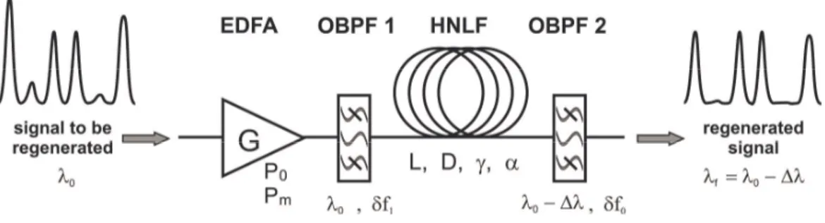
2. Principle and set-up

The set-up of the single stage Mamyshev regenerator under study is described in Fig 1. The signal to be regenerated is first amplified in order to reach an optimum average power Pm

(corresponding to a peak power P0 for ‘1’ pulses). An optical bandpass filter (OBPF), centred

at the signal wavelength

λ

0 and characterized by its spectral full-width at half maximum

(FWHM)

δ

f1 is also used to reduce the ASE noise power [16]. A spectral broadening is then

achieved through the SPM effect occuring during the propagation in a highly non-linear optical fiber (HNLF) with a length L. The broadened spectrum is finally partially sliced by a second OBPF shifted by

∆λ

. The spectral bandwidth of this second filter

δ

f0, which

determines the output pulse width, is then fixed according to the initial pulse properties.

Fig. 1. Set-up of the single stage Mamyshev regenerator. Erbium Doped Fiber Amplifier (EDFA), Optical BandPass Filter (OBPF), Highly Non-Linear Fiber (HNLF).

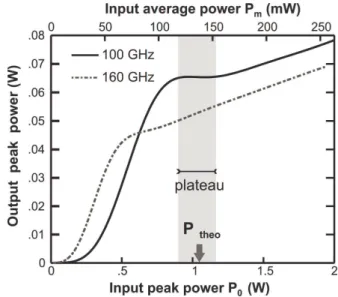
In Ref. [14] the authors have shown that, according to the system parameters (L, P0

and

∆λ

), three different regimes of transfer function ( Pout = f ( Pin ) ) can be observed : a

transfer function (TF) characterised by a plateau (B regime), by a continuously increasing behaviour (C regime) or by a non-monotonic regime (A regime). The transfer function associated with the plateau zone of the B regime (and corresponding to an input peak-power

Ptheo ) has been considered as the most suitable to achieve an efficient regeneration process,

mainly due to its capacity to equalize pulse-to-pulse peak-power fluctuations.

Our regenerator is based on a HNLF with a length L of 3500 m, a non-linear coefficient

γ

of 8.4 W-1.km-1, a dispersion D of -0.7 ps.km-1.nm-1 and a linear loss coefficient

α

of 0.6 dB.km-1. We have included in our simulations the ASE noise introduced by the

erbium doped fiber amplifier (EDFA) by taking into account a noise figure Nf = 4 dB.

Following the method detailed in [14], we have calculated the TF thanks to the propagation of a single Gaussian pulse having a temporal FWHM of T0 = 6.25 ps, which corresponds to the

pulses used in a classical 40-Gbit/s return-to-zero-25% (RZ-25) optical telecommunication system.

Our simulations have been computed by means of the software VPI WDM Transmission Maker and rely on the numerical integration of the non-linear Schrödinger equation by a split-step Fourier method. Note that polarisation mode dispersion (PMD) as well as other higher-order non-linear effects (Raman, Brillouin or self-steepening contributions) have been neglected in our simulations.

OBPF 2 is a Gaussian filter with a spectral width

δ

f0 = 70 GHz and a spectral offset

∆λ =

160 GHz. For an initial 4-th order supergaussian OBPF with a spectral width

δ

f1 = 100

GHz (OBPF 1), we obtain a B-like TF (Fig. 2, solid line), with a plateau around Ptheo = 1.05

W. Let us note that we can easily obtain other TF types by simply adjusting

δ

f1. Indeed, by

changing the spectral width of the initial filter, we also modify the initial temporal width of the pulses entering the HNLF. Given the dependence of TF with the initial pulse properties, this leads to noticeable changes of the TF. For example, if

δ

f1 = 160 GHz (mixed line), we

obtain a C-like TF and by using narrower filters, an A-like TF could also be achieved.

Fig. 2. Transfer function of a single-stage regenerator. Evolution of the output peak-power versus the input power for two different spectral widths of OBPF 1 (

δ

f1 = 100 GHz and

δ

f1 =

160 GHz, solid black line and mixed line, respectively). The input average power corresponds to the average power of a 40-Gbit/s pseudo-random binary sequence (PRBS) signal.

3. Performance of the single-stage regenerator

In this part, we aim to quantify the regenerative capacity of the B-like single-stage Mamyshev regenerator described in the above section. The transfer function is usually built by computing the response of the regenerator to an input single pulse. However, in order to fully characterize the performance of a regenerator, a stream of pulses (namely a pseudo-random binary sequence (PRBS)) has to be taken into account. In that context, the usual parameter widely used to evaluate the signal quality is the Q-factor [2] : Q = (V1 – V0) / (

σ

1 –

σ

0), with

V1 and V0 the average electrical voltage of the ones and zeros respectively at the detection

instant, and

σ

1 and

σ

0 the corresponding standard deviations. A good estimation of the

performance of our regenerator will be the Q-factor improvement defined as the ratio between the input and output signal Q-factor (or equivalently the difference when expressed in dBs). On the other hand, the Q-factor parameter, obtained in the electrical domain, often hides the physical meaning of the signal degradation and consequently, this data itself is not enough to get a precise understanding of the degradation affecting the pulse train. So in order to complete the analysis, we will also get interested in the statistical properties of the optical signal, i.e. its temporal pulse width, its peak-power, its temporal position and its extinction-ratio.

3.1. Initial input pulse properties

In this section, we shall first study the features of the degraded 40-Gbit/s PRBS signal used at the input of the regenerator.

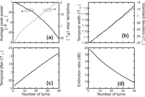
In order to model realistically the signal degradation [21] and to maintain an affordable computation time, we have numerically propagated a (211-1)-long 40-Gbit/s RZ-25 PRBS signal in the recirculating loop system represented in Fig. 3(a). The FWHM of the pulses is 6.25 ps, the initial extinction ratio (defined by the ratio between the ‘1’ peak-power and the ‘0’ level) is 20 dB and the initial signal average power launched into the loop is 1 dBm. The loop is made of 100 km of standard single mode fiber (SMF) with an anomalous dispersion of 16 ps/km/nm, a dispersion slope of 0.08 ps/km/nm2, a non-linear coefficient of 1.3 W-1.km-1 and an attenuation of 0.2 dB/km. Dispersive effects are compensated by 16 km of dispersion compensating fiber (DCF) with a normal dispersion of -100 ps/km/nm, a

dispersion slope of -0.5 ps/km/nm2, a non-linear coefficient of 5.2 W-1.km-1 and an attenuation of 0.6 dB/km. This compensating fiber is preceded and followed by erbium doped fiber amplifiers (EDFA) with gains GA = 14 dB and GB = 15.6 dB, respectively. Both amplifiers are

followed by a 4-th order supergaussian OBPF with a spectral width of 400 GHz in order to partly remove the ASE noise introduced by the amplifiers. Finally, the 40-Gbit/s receiver module is preceded by a supergaussian OBPF with a FWHM of 160 GHz.

Fig. 3. (a) Scheme of the loop system used to model the degradation of the 40-Gbit/s PRBS signal during the propagation. (b) Evolution of Qin as a function of the number of round

trips. (c) Optical eye-diagrams for three different levels of degradation ( Qin = 24, 6 and 3.3,

subplots 1, 2 and 3 respectively )

Fig. 3(b) represents the evolution of the optical signal quality factor Qin as a function

of the number of turns completed into the loop. As expected, the Q-factor progressively decreases due to the cumulative impairments occurring during the propagation, namely the accumulation of in-band ASE noise and combined effects of chromatic dispersion and non-linear effects (intrachannel cross-phase modulation and four-wave mixing [3]). Consequently,

without any regeneration, only 20 round trips (2000 km) could be covered before falling down to the transmission limit corresponding to Qin = 6. Let us note that the present loop is not

fully-optimized to its best performances and that some pre-chirp/post-chirp could still enhance the transmission distance.

In the following of the paper, we will particularly investigate the evolution in the regenerator of three different levels of Q-factor at the input, i.e. Qin = 24 (signal of excellent

quality corresponding to a 200 km propagation distance), Qin = 6 (limit transmission signal

quality [2] ) and Qin = 3.3 (signal of extremely poor quality after 3500 km of propagation

which can only be used in presence of forward error correction (FEC)). Eye-diagrams corresponding to these three levels of degradation are presented in Figs. 3(c) and clearly reveal that the degradation of the input Q-factor has multiple sources: amplitude jitter, timing-jitter as well as an extinction ratio decrease.

In order to get a more precise quantitative description of the degraded 40-Gbit/s PRBS signal, we now consider in Fig. 4 the average values and root-mean square (rms) deviations of several signal key parameters.

As can be seen in Fig. 4(a-b), the amplitude jitter

σ

Ain (rms deviation of distribution of

the peak power of the pulses) as well as the temporal jitter

σ

Tin (rms deviation of distribution

of the central pulse position as defined by its highest peak-power) strongly increase during the propagation to reach after 4000 km, 20% of the pulse width and peak power, respectively. The effects of the ASE accumulation and the ghost-pulses generation are also apparent through the significant decrease of the extinction ratio (Fig 4(d)) which drops from 10 dB after 40 round trips. We can finally note in Fig. 4(b) that during the propagation, the temporal pulse width increases, with a rise as high as 20 % of its initial value after 4000 km, leading to a decrease of the average pulse peak-power. We will discuss in more details the implications of those fluctuations in section 4.3.

Fig. 4. Statistics of the 40-Gbit/s PRBS signal as a function of propagation distance (or equivalently number of turns n). (a) Evolution of the average peak-power (solid black line, left, normalized by the initial peak-power Pin) and the amplitude jitter (grey dotted line, right,

defined as the standard deviation of the peak-power distribution, normalized by the average peak-power) (b) Evolution of the temporal FWHM Tn (left, solid black line) and its

standard deviation (right, normalized by the temporal width Tn, grey dotted line).

(c) Temporal jitter (defined as the standard deviation of the distribution of the central position of the pulse, normalized by the FWHM average temporal width Tn at turn n) (d) Evolution of

the extinction ratio.

3.2. Performance of the regenerator and optimum working point

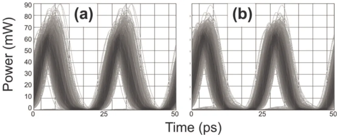
We first test our regenerator on a degraded signal with Qin = 6. Eye-diagrams after

regeneration are plotted in Figs. 5 for two regenerator input values of the average powers Pm

(called the working power (WP)). As can be seen, in both cases, the regenerator improves very efficiently the extinction ratio of the pulse train and also tends to limits the amplitude jitter. The eye is then clearly more opened than in Fig. 3(c2), despite the presence of some additional timing jitter. We can also make out that the WP largely influences the quality of the output pulse, with better results obtained at a WP of 180 mW.

Fig. 5. Optical eye-diagrams after regenerator for Qin = 6 for two different working powers.

(a) WP = 130 mW (b) WP = 180 mW.

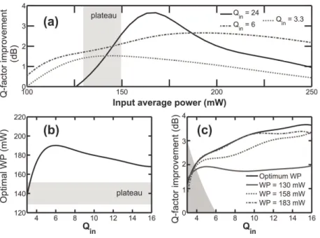
In order to quantify the impact of the regenerator, we measure the improvement of the signal in terms of Q-factor enhancement [16], i.e. the ratio Qout / Qin where Qout is the quality

factor at the output of the regenerator. We present in Fig. 6(a) the Q-factor improvement as a function of the WP for three different levels of degradation. Let us notice that studying the Q factor improvement is not sufficient to quantify the performances of a regenerator [22]. However, in the context of our study, where we focus on the physical mechanism of the regeneration process, the Q-factor is a convenient parameter to quantify the quality of the signal after regeneration. First and in disagreement with the TF approach described in Fig. 2, we can observe, for Qin = 24 and Qin = 6, that the optimal regeneration is not obtained on the

plateau (around Ptheo), but for a higher WP. This observation is quite surprising but consistent

with the behaviour previously highlighted in Ref. [12, 16]. We can also make out that the signal quality improvement strongly depends on its initial degradation. Indeed, for a high Qin

(Qin = 24), the optimum regeneration is achieved on a relatively narrow input power range and

reaches 3.5 dB for an input average power of 170 mW. On the contrary, for a more degraded signal (Qin = 6), the performances of the regenerator fortunately do not exhibit such a strong

Fig. 6. Regenerator performances. (a) Q-factor improvement as a function of the WP for three different levels of degradation ( Qin = 24, 6 and 3.3, solid black line, mixed line and grey

dotted line, respectively). (b) Optimal WP versus the Qin. In Figs (a) and (b), the shaded

areas correspond to the plateau zone (see Fig. 2(a)). (c) Q-factor improvement versus Qin

for different WP : optimum WP (solid black line), WP of 130 mW, 158 mW and 183 mW (solid grey line, dotted grey line and mixed grey line, respectively), corresponding to input peak-powers of 1 W, 1.2 W and 1.4 W, respectively. The shaded area denotes the zone where the regenerated Q-factor is below 6.

We have also plotted in Fig. 6(b) the evolution of the optimal average WP as a function of Qin. We can see that the optimum power has to be tuned above the plateau area

between 140 and 190 mW and depends on the level of degradation, with a decrease of the power for low Qin. We will give some explanations about such a dependence in the next

section.

The next plot, Fig. 6(c), shows the Q-factor improvement as a function of the input Q-factor Qin for several values of WP. For comparison, we have plotted in solid black line the

maximum feasible improvement; that is to say for each value of Qin, the maximum of Q-factor

improvement at the optimum WP. But in practice, it could be easier to fix the amplifier to a given WP, no matter what Qin is. This is the reason why we have also plotted the results

corresponding to a WP of 130, 158 and 183 mW in solid grey line, dotted grey line and mixed grey line, respectively. It is then important to notice that in all cases, we have improved the signal quality, but the value of this improvement could be significantly different. For

example, the choice of a working power of 130 mW (corresponding to the value of the plateau

Ptheo) clearly appears to lead to a non-optimum regeneration whereas a working power of

183 mW is closer to the all-cases optimum regeneration.

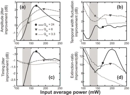
In order to better understand the behaviours related above, we now quantify the action of the 2R Mamyshev regenerator in terms of statistics. In Figs. 7, we study the modification of the statistics induced by the regenerator on the 40-Gbit/s PRBS signal as a function of the input average power for three different levels of degradation (Qin = 24, 6 and 3.3, solid black

line, mixed line and grey dotted line, respectively). For memory, the optimal WP giving the highest Q-factor improvement found in part 3.2, Fig. 6 are indicated by means of a black circle, a grey triangle and a grey square for Qin = 24, 6 and 3.3, respectively.

Let us first study the benefits provided by our regenerator in terms of amplitude jitter reduction. We define the amplitude jitter improvement as the ratio between the input and output amplitude jitter

σ

Ain /

σ

Aout (or the difference when expressed in dBs). We can see from

Fig. 7(a) that for a WP above 125 mW, the regenerator always leads to an amplitude jitter improvement, with a maximum as high as 2.6 dB of improvement for weakly degraded signals ( Qin = 24).

We have also calculated the action of the regenerator on the temporal width fluctuations by defining the temporal width fluctuations improvement as the ratio between the input and output rms deviation of the pulse width distribution σ∆Tin / σ∆Tout. We can see in

Fig. 7(b) the beneficial impact of the regenerator [13]. The output pulse width fluctuations strongly decreases whatever WP for Qin=6 and Qin=3.3 and decreases if WP > 130 mW for

Qin = 24. Note that this regeneration of the temporal pulse width is a specific benefit of the

Mamyshev regenerators compared with other usual 2R techniques. This is due to the presence of the output filter whose role is to shape the pulse profile at the output of the regenerator.

If we now have a look at the regenerator impact in terms of timing jitter, we can calculate

σ

Tin /

σ

Tout. We then observe in Fig. 7(c) that the regenerator introduces an extra

temporal jitter [15] which always degrades the input signal by inducing an average of 1 dB penalty whatever the WP is.

Finally, we have plotted the ER enhancement defined as ERout / ERin in Fig. 7(d).

These results show that our regenerator leads to a significant ER improvement for any input average power between 100 and 250 mW.

Fig. 7. Statistics regarding the single-stage regenerator impact on a 40-Gbit/s degraded signal for three levels of degradation (input Q-factor of 24, 6 and 3.3, solid black line, mixed line and grey dotted line, respectively) as a function of the regenerator input average power (a) Amplitude jitter improvement (b) Temporal-width fluctuations improvement (c) Timing jitter improvement and (d) Extinction-ratio improvement. The optimal WP

found in part III.B, Fig. 5 are indicated by means of a black circle, a grey triangle and a grey square for Qin = 24, 6 and 3.3, respectively. The shaded areas correspond to the plateau zone

(see Fig. 2).

4. Explanations for the choice of the working power

In the last subsection, thanks to the statistical analysis completed on the 40-Gbit/s PRBS signal, we now better understand the origin of the Q-factor improvement provided by the Mamyshev regenerator as a function of the input average power. However and in agreement with reference [16], we observed the non intuitive phenomenon that the effective optimal WP does not necessary correspond to the range of powers at which the TF exhibits a plateau area around Ptheo. It is the reason why, in the present section, we will try to link the 40-Gbit/s

PRBS Q-factor improvement approach and its statistical analysis with the TF approach computed by the propagation of a single Gaussian pulse. We will then propose and discuss explanations about the difference between the usual theoretical WP Ptheo and the effective

optimal WP where the Q-factor improvement is maximal as well as an explanation to the dependence of Q factor improvement over Qin.

4.1. Induced timing jitter and output temporal width fluctuations

In reference [14], the aim of the paper was mainly focus on both the peak-power equalisation and the extinction ratio-improvement by means of the single-pulse TF optimisation. Following a similar approach, we can calculate the temporal changes affecting the output Gaussian pulse properties as a function the input power. Let us note that this study is different from the results dealing with the nominal soliton number parameter presented in [14] (cf. Fig. 5 of this reference) where the regenerator properties (fiber length and filter offset) where constantly adjusted in order to operate on the plateau area.

Results plotted in Fig. 8(a) show that, in the case of a single pulse propagation, the fluctuations of the output temporal width are maximum in the range of power corresponding to the plateau area, which has been recently confirmed by experimental FROG measurements [9]. Let us however relativize the impact of those fluctuations: as can been seen in Fig. 7(b), the 40-Gbit/s statistical study outlines a clear improvement of the regenerated pulse train in terms of temporal width fluctuation. In other words, the fluctuations induced by the regenerator are largely compensated for by the intrinsic enhancement provided by the Mamyshev method [13] and are consequently not sufficient to explain the WP offset.

Fig 8. (a) Evolution of the temporal width

∆

Tout of the output pulse as a function of the input

peak-power (b) Time delay

δ

T introduced by the single-stage regenerator (c) Derivative

of the time delay. Results are normalised by the input pulse width T0. The grey area represents

the plateau zone. The sampling time is 24 fs (.004 T0).

We also got interested in the delay potentially introduced by the regenerator (Fig 8(b)). Note that the sign of the delay depends on the spectral offset sign. Changing the sign of the spectral offset in –

∆λ

will lead to an opposite time delay. Once again, we notice that the

temporal delay exhibits maximum variations in the plateau zone. But here, the most interesting point does not lie in the absolute value of the delay in itself, but rather in its fluctuations, which directly induce timing jitter. Figure 8(c) shows the amplitude-derivative of the time-delay as a function of input power. We can clearly observe that this function is remarkably maximum at the plateau zone and that the time delay fluctuations and thus the extra induced timing jitter could be minimised by at least a factor four for a higher WP (for example 180 mW) which could partially explain the behaviour observed in Fig. 7 for Qin = 24

and Qin = 6 where, as the input signal is of a pretty good quality, the optimum WP

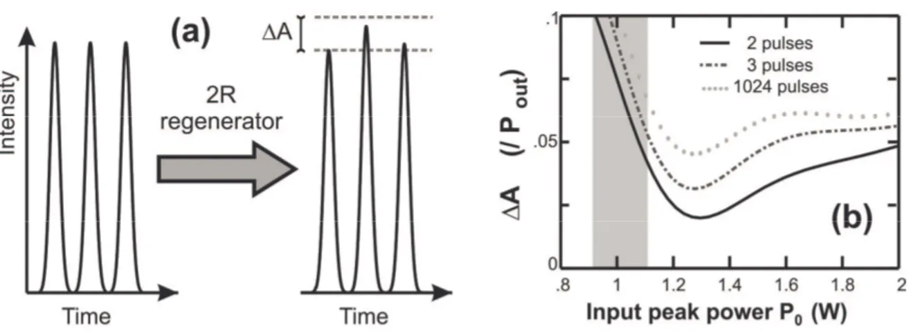
4.2. Pulse-to-pulse overlapping induced amplitude jitter

Besides this first aspect, another key point we got interested in is the effect provided by the pulse-to-pulse overlapping occurring inside the regenerator due to the chromatic-dispersion induced pulse broadening [23]. To this aim, we study, in a similar manner as in references [14, 17], the amplitude jitter induced by the cross-phase modulation occurring during the adjacent pulse-to-pulse overlapping (what is called “collision” in ref. [14]) in a sequence of 2 or 3 pulses propagating in the regenerator. We have also considered a PRBS of 1024 pulses which includes all the possible combinations up to tens consecutive pulses. Using longer sequences has not lead to noticeable changes. In order to be solely sensitive to the impact of this overlapping, we have considered an initial signal with an infinite ER and we have neglected the ASE introduced by the EDFA. For each input peak-power, we have computed the difference

∆

A (see Fig. 9(a)) between the two peak-power extrema obtained in

the output pulse sequence. The quantity

∆

A qualifies the amplitude jitter induced by the

intra-channel interactions. Results are normalized by the average output pulse peak-power and are plotted in Fig. 9(b).

Fig. 9. Effects of pulse-to-pulse overlapping in the optical regenerator. (a) Principle and notations (b) Peak-power fluctuations at the output of the regenerator (normalized by the

average output peak-power) for a sequence of 2 (black solid line), 3 (mixed line) and 1024

As in the previous timing-jitter study, the degradation due to overlapping is more pronounced on the plateau zone than at higher working power: the minimum of induced amplitude jitter is observed around 1.3 W, corresponding to a 40-Gbit/s PRBS average power of 170 mW. These conclusions then clearly explain the WP offset observed in Fig. 7 for the

Qin = 24 initial pulse train where the optimal input average power mostly corresponds to the

minimum of amplitude jitter degradation introduced by the regenerator itself which, with the intrinsic enhancement provided by the Mamyshev method, participates to reach a maximum amplitude jitter improvement. In other words, for input signals of good quality, the main factor affecting the 2R performance is the pulse-to-pulse overlapping induced amplitude jitter. For a poor quality signal (Qin = 3.3), the interpretation is still more complex.

Let us finally note that it could be possible to significantly reduce the impact of pulse-to-pulse overlapping by an appropriate choice of the regenerator parameters (L,

∆

f), as well as

the initial OBPF 1 (as it determines the duty-cycle of the signal). More precisely, using a lower nominal soliton number parameter (as defined in ref [14]) would allow us to partly eliminate this deleterious pulse overlapping [14]. However such a change in the regenerator features is usually at the cost of the ER. So, a trade-off between the ER improvement and the collision-induced amplitude jitter reduction has to be found. Such a study is however beyond the scope of the present paper.

4.3. Impact of temporal width change

In summary, from the conclusions outlined in the last subsections 1 and 2, it could be efficient to use a WP higher than the plateau power in order to minimise the timing jitter intrinsically induced by the regenerator, as well as the amplitude jitter induced by the pulse-to-pulse overlapping.

In this subsection, we highlight the strong impact of the initial temporal pulse fluctuations, leading to an additional source of amplitude jitter. Statistics of the input signal presented in Fig. 4 have revealed that the temporal width undergoes some non-negligible fluctuations (both in terms of average value and standard deviation). This can have a large impact on the regenerator behaviour. Indeed, it has been previously demonstrated [11, 14, 19] that, contrary to NOLMs or other 2R regenerating devices, temporal width of the incoming

pulses is a crucial parameter in the sense that the transfer function strongly depends on this parameter. In this context, considering a single TF relying on well defined 6.25 ps Gaussian pulses can be viewed as an inaccurate approximation.

In order to better apprehend the impact of this temporal width distribution, we have plotted in Figs. 10(a) the distribution of the temporal width of the 40-Gbit/s PRBS signal for three levels of degradation (Qin = 24, 6 and 3.3, (a1), (a2) and (a3) respectively).

Fig. 10. Impact of the statistical evolution of the temporal width for three different values of

Qin of 24, 6 and 3.3 (subplots 1, 2 and 3 respectively). (a) Statistical distribution of the

temporal pulse width of the 40-Gbit/s signal (b) statistical TF for input pulses with a temporal width distribution corresponding to Figs. (a). Black line corresponds to the average peak power of the pulse train and the shaded area corresponds to the whole output peak powers possibilities.

We have plotted in Figs. 10(b) the transfer functions obtained by taking into account the whole distribution of temporal pulse width. In order to do that, we have taken an input series of 256 Gaussian pulses with a temporal width distribution similar to that exposed in Figs. 10(a) (same average, same deviation). Note that the input pulses have been separated by an empty time slot in order to remove pulse-to-pulse overlapping induced effects. All the initial pulses have the same initial energy. In other words, the fluctuations of temporal width are directly associated with fluctuations of the input peak power. The output peak power (black solid line) represents the output pulse train average peak-power. It can be seen that in

all cases, a TF exhibiting a plateau is achieved. However, the change in the average temporal width leads to a slight shift in the value of the plateau which increases from an input average power of 140 mW for Qin = 24 up to a 160 mW for Qin = 3.3. But, the most striking point is

undoubtedly the significant fluctuations in the TF. We have plotted as shaded area the whole values of the output peak-powers. For high Qin, as the deviation of the temporal width is not

high, the fluctuations are not severe. But for more degraded signals, the temporal width fluctuations may lead to a non-negligible additional source of amplitude jitter in the regenerated signal. It is then remarkable that the output amplitude fluctuations are reduced when increasing the input average power, in agreement with the trends observed in Fig. 7(a). This phenomenon underlines again the key role played by the amplitude jitter improvement in the choice of the optimal input power and thus the trend to operate with a WP higher than the plateau area.

Let us however note that the choice of taking all the initial pulses with the same energy represents an approximation, since in reality temporal fluctuations are also not strictly correlated with peak-power fluctuations. More realistic simulations could be carried out by use of more sophisticated methods such as multicanonal Monte-Carlo approach [18], but such an analysis is beyond the scope of the present paper.

4.4. Impact of Extinction Ratio improvement

The three previous subsections have provided us several trends which help us to better understand the choice of the optimal WP for high or intermediate qualities of initial signals (Qin = 24 or Qin = 6). We have indeed shown that amplitude- and timing- jitter reductions are

the key issues that govern the choice of the WP.

On the contrary, for a highly degraded signal (Qin = 3.3), the choice of the WP

becomes a trade-off between the ER improvement and the amplitude jitter reduction. Indeed, in Fig. 7(d), as the evolution of the ER improvement is quite flat for Qin = 6 between 125 and

225 mW, the performances of the regenerator is weakly influenced by the ER improvement but rather governed by the amplitude- and timing- jitters reductions. On the opposite, variations as high as 4 dB can be observed for Qin = 3.3 in the same range of power. The Qin =

3.3 ER enhancement being a decreasing function with respect to WP, a large improvement of the ER will consequently lead to a lower WP with a minimum of 130 mW corresponding to

the limit of a non degradation of the initial amplitude jitter (

σ

Ain /

σ

Aout = 0 dB). This

behaviour which explains the decrease of the optimal WP observed for Qini < 6 in Fig. 6(b).

5. Performance of the double-stage regenerator

Let us first recall that in order to restore the initial signal wavelength, a second wavelength-converter stage is required. We now study the performance of such a double stage regenerator.

5.1. Principle and set-up

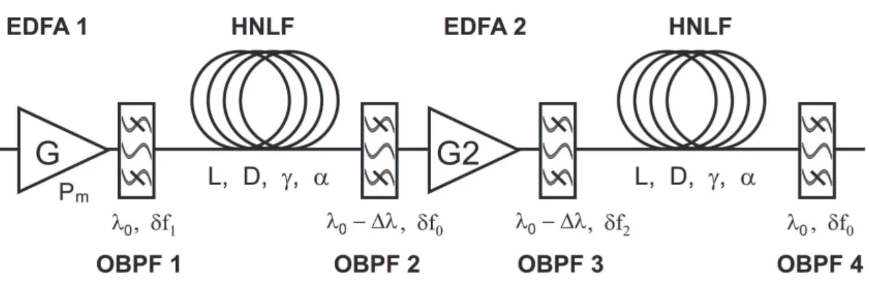
The set-up based on a two-stage Mamyshev regenerator is presented in Fig. 11. Two single stage regenerators are then concatenated. In order to have a device compatible with a bidirectional use [7, 8], we have used the same HNLF properties in the two stages of regeneration.

Let us outline that the OBPF 1 and 3 can be identical, in which case a configuration B + B is obtained. But they can also be different, leading to various arrangements such as C + B or A + B, or any other type of association. This opens many possibilities, but a complete study of those combinations is out of the scope of the present paper. We will then only focus on the B + B arrangement.

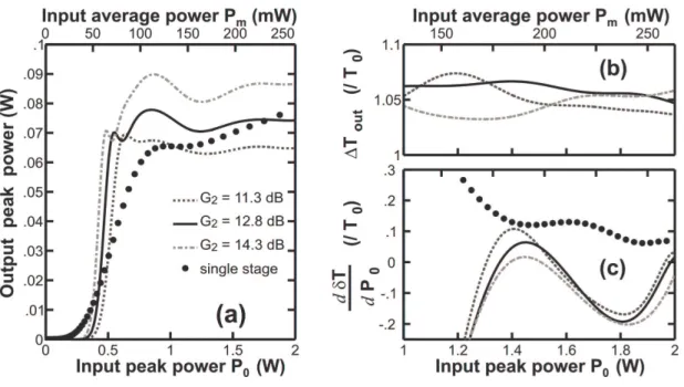
The TF obtained by this concatenation is plotted in Fig. 12 for several values of the intermediate amplifier gain G2 (noise figure of the amplifier Nf = 4 dB). We have plotted the

results for three different gains of 11.3 dB, 12.8 dB and 14.3 dB (dotted line, solid black line and mixed line, respectively). We can see that the 12.8 dB gain leads to a good power equalisation (Fig. 12(a)) and limits the impact of the extra-temporal jitter (Fig. 12(c)). Indeed, temporal jitter introduced by the first regenerator is partly compensated by the second one. Let us however outline that the time delay introduced by each regenerator do not add and that the concatenation of two regenerator leads to a more complex dynamics [19]. Regarding the output pulse temporal width fluctuations (Fig. 12(b)), they are quite limited.

We can also see from Fig. 12(a) that the TF is now steeper with a larger plateau and an enhanced ER compared to a single stage B (black circles).

Fig. 12. Characteristic of a double-stage regenerator. Evolution of the output pulse properties according to the input power for three different gains G2 = 11.3, 12.8 and 14.3 dB (dotted line,

solid black line and mixed grey line respectively). Results are compared with results of the single-stage regenerator (black circles) (a) Evolution of the output peak-power. (b) Evolution of the temporal width

∆

Tout of the output pulses (c) Derivative of the time

delay versus the input peak-power. Results (b) and (c) are normalised by the input pulse width

5.2. Q-factor improvement

We have plotted in Fig. 13 the performances of the double stage regenerator in terms of Q-factor improvements. Compared to the results described in section 3.2 Fig. 6, several differences can be outlined. First, we can see in Fig. 13(a) that the regeneration input power range is broader than for a single stage regenerator.

Fig. 13. Double-stage regenerator performances. (a) Q-factor improvement according to the WP for three different levels of degradation (same convention as Fig. 4(a)) (b) Optimal WP versus the input Q-factor. (c) Q-factor improvement relative to the input Q-factor for different WP : optimum working power (solid black line), working power of 183 mW (mixed grey line), Results of the two-stage regenerator are compared with the results of a single-stage configuration (dotted grey line).

We can also observe that the dependence (Fig. 13(b)) of the optimal WP versus the initial degradation is less pronounced than in the single stage configuration, which is beneficial for system implementation.

We can also make out from the comparison of Figures 6(c) and 13(c) that for a low degraded signal, a double stage device is slightly less efficient than a single-stage configuration. But for lower Qini (Qini < 10), the double stage leads to regeneration

enhancements. For example, the regeneration (Qout > 6) of a degraded signal with a quality

factor as low as 3.3 becomes possible. Let us however here recall that the Q-factor data must be handled with special care in the case of optical regenerators [22] and that a link with bit error rates is not straightforward in that context.

5.3. Statistical impact of the double stage regenerator

We carry out in this sub-section similar study as the one presented in part 3.2. Results are plotted in Fig. 14 and the general trends are similar to the results obtained for a single stage configuration.

Fig. 14. Statistics regarding the double-stage regenerator impact on a degraded signal for three levels of degradation (input Q-factor of 24, 6 and 3.3, solid black line, mixed line and grey dotted line respectively). Same conventions as Fig. 7. Optimal working points are the WP found Fig. 13.

As compared with the quantitative results obtained for a single stage, we can note the followings points. First, the amplitude jitter reduction capacity is improved, which is

consistent with the enhanced plateau observed Fig. 12(a). Then, improvement of the temporal width fluctuations is also observed, in agreement with Fig. 12(b). The extinction ratio improvement is also significantly enhanced, in agreement with the stepper TF observed in Fig. 12(a). Regarding the timing jitter introduced during the regeneration, the double stage scheme does not seem to significantly further degrade this data. We could have expected from Fig. 12(c) a reduction of the timing jitter, but one has also to take into account the other sources of timing jitter such as intra channel pulse-to-pulse overlapping. As a consequence, for a low degradated initial signal, the extra timing jitter is slightly higher in the double stage configuration than in the single stage, which can partly explain the performance degradation of the double stage regenerator for Qin above 10.

6. Conclusion

We have numerically studied the performances of a 2R Mamyshev optical regenerator used in a 40-Gbit/s RZ-25 system. Based on this given configuration, we have outlined several key elements of Mamyshev regenerators which have to be taken into account into the set-up design : the induced timing jitter, the temporal width fluctuations and the pulse-to-pulse overlapping. Impact of the fluctuations of the temporal width of the initial pulses has also been outlined. Those generic elements enable us to physically explain the differences which can be observed between the general predictions of Provost et al. in Ref. [14] and the working power which is required to achieve optimum eye opening for our given configuration.

We have also used a statistical approach to describe quantitatively the role of the regenerator and to explain the dependence of the performance on the degradation of input signal.

We have finally proposed and analyzed a two-stage configuration where the deleterious impact of the timing jitter can be partly minimized. Improvement of amplitude jitter and extinction-ratio is demonstrated and the distance of propagation can be improved by using such a double-stage in front of the receiver. A further step will be the investigation of the regenerator capacity in a loop configuration but let us note that the requirements of such a regenerator will be quite different : due to the periodic use, improvements of the ER and amplitude jitter will not be so severe as amplitude jitter and noise will not develop so heavily. On the contrary, in a loop configuration, issues such as timing-jitter reduction and collisions

induced-effects [14] will become even more crucial. Given those given specific requirements, we anticipate that further optimization process adapted to in-line regeneration will be necessary.

Acknowledgments

This research was supported by the Agence Nationale de la Recherche (FUTUR project). We acknowledge fruitful discussions with B. Patin (Institut Carnot Bourgogne, France). We are very grateful to I. Joindot and M. Joindot (FOTON, France) for their comments on the manuscript.

References

[1] D. Rouvillain, P. Brindel, F. Seguineau, L. Pierre, O. Leclerc, H. Choumane, G. Aubin, and J. L. Oudar, Electron. Lett. 38 (2002) 1113-1114.

[2] G. P. Agrawal, Fiber-Optic Communication Systems: Wiley-Interscience, 2002. [3] R. J. Essiambre, B. Mikkelsen, and G. Raybon, Electron. Lett. 35 (1999) 1576-1578. [4] N. J. Doran and D. Wood, Opt. Lett. 13 (1988) 56-58.

[5] E. Ciaramella, F. Curti, and S. Trillo, IEEE Photon. Technol. Lett. 13 (2001) 142-144. [6] P. V. Mamyshev, "All-optical data regeneration based on self-phase modulation effect," in European Conference on Optical Communication, ECOC'98, Institute of Electrical and Electronics Engineering, Madrid, Spain, 1998, pp. 475-476.

[7] M. Matsumoto, Opt. Express 14 (2006) 11018-11023.

[8] L. Provost, F. Parmigiani, C. Finot, P. Petropoulos, and D. J. Richardson, "Self-Phase Modulation-based 2R optical regenerator for the simultaneous processing of two WDM channels " in CLEO Europe, Munich, 2007.

[9] L. Provost, C. Finot, K. Mukasa, P. Petropoulos, and D. J. Richardson, "Generalisation and experimental validation of design rules for self-phase modulation-based 2R-regenerators," in Optical Fiber Conference, OFC 2007, Anaheim, USA, 2007, p. OThB6.

[10] C. Finot, S. Pitois, and G. Millot, Opt. Lett. 30 (2005) 1776-1778.

[11] M. Rochette, L. B. Fu, V. G. Ta'eed, D. J. Moss, and B. J. Eggleton, IEEE J. Sel. Top.

Quantum Electron. 12 (2006) 736-744.

[12] T.-H. Her, G. Raybon, and C. Headley, IEEE Photon. Technol. Lett. 16 (2004) 200-202.

[13] B. E. Olsson and D. J. Blumenthal, J. Lightwave Technol. 20 (2002) 1113-1117. [14] L. Provost, C. Finot, K. Mukasa, P. Petropoulos, and D. J. Richardson, Opt. Express

15 (2007) 5100-5113.

[15] J.-T. Mok, J. L. Blows, and B. J. Eggleton, Opt. Express 12 (2004) 4411-4422.

[16] T. N. Nguyen, M. Gay, L. Bramerie, T. Chartier, and J. C. Simon, Opt. Express 14 (2006) 1737-1747.

[17] T. I. Lakoba and M. Vasilyev, Opt. Express 15 (2007) 10061-10074.

[18] T. I. Lakoba and M. Vasilyev, "Multicanonical Monte-Carlo simulations of the dynamix power transfer characteristic of an all-optical 2R regenerator," in Nonlinear

Photonics 2007, Québec, 2007, p. JWA6.

[19] S. Pitois, C. Finot, and L. Provost, Opt. Lett. 32 (2007) 3262-3264. [20] M. Matsumoto, IEEE Photon. Technol. Lett. 19 (2007) 273-275.

[21] L. K. Wickham, R. J. Essiambre, A. H. Gnauck, P. J. Winzer, and A. R. Chraplyvy,

IEEE Photon. Technol. Lett. 16 (2004) 1041-1043.

[22] M. Gay, L. Bramerie, J. C. Simon, V. Roncin, G. Girault, M. Joindot, B. Clouet, S. Lobo, S. Feve, and T. Chartier, "2R and 3R optical regeneration : from device to system characterization," in European Conference on Optical Communication, ECOC Cannes, 2006.