Online Demand Estimation of Geographical and Non-Geographical Distributed Demand Pattern in Water Distribution Networks

HAL Id: hal-01745358

https://hal.archives-ouvertes.fr/hal-01745358

HAL is a multi-disciplinary open access archive for the deposit and dissemination of sci-entific research documents, whether they are pub-lished or not. The documents may come from teaching and research institutions in France or abroad, or from public or private research centers.

L’archive ouverte pluridisciplinaire HAL, est destinée au dépôt et à la diffusion de documents scientifiques de niveau recherche, publiés ou non, émanant des établissements d’enseignement et de recherche français ou étrangers, des laboratoires publics ou privés.

Water Distribution Networks

Nhu Cuong Do, Angus Simpson, Jochen Deuerlein, Olivier Piller

To cite this version:

Nhu Cuong Do, Angus Simpson, Jochen Deuerlein, Olivier Piller. Online Demand Estimation of Geographical and Non-Geographical Distributed Demand Pattern in Water Distribution Networks. CCWI 2017 - Computing and Control for the Water Industry, Sep 2017, Sheffield, France. 8 p., �10.15131/shef.data.5364133.v1�. �hal-01745358�

Online Demand Estimation of Geographical and Non-Geographical

Distributed Demand Pattern in Water Distribution Networks

Nhu Cuong Do1_{, Angus R. Simpson}2_{, Jochen W. Deurelein}3_{, Olivier Piller}4

1,2 _{School of Civil, Environmental and Mining Engineering, University of Adelaide, Adelaide SA}

5005, Australia.

3 _{3S Consult GmbH, Karlsruhe, Germany}

4 _{Irstea, UR ETBX, Department of Waters, France, Bordeaux}

1_{nhu.do@adelaide.edu.au}

ABSTRACT

The issue of demand calibration and estimation under uncertainty is known to be an exceptionally difficult problem in water distribution system modelling. In the context of real-time event modelling, the stochastic behaviour of the water demands and non-geographical distribution of the demand patterns makes it even more complicated.

This paper considers a predictor – corrector approach, implemented by a particle filter model, for solving the problem of demand multiplier factor estimation. A demand forecasting model is used to predict the water demand multiplier factors. The EPANET hydraulic solver is applied to simulate the hydraulic behaviour of a water network. Real time observations are integrated via a formulation of the particle filter model to correct the demand predictions.

A water distribution network of realistic size with two configurations of demand patterns (geographically distributed demand patterns and non-geographically distributed demand patterns) are used to evaluate the particle filter model. Results show that the model is able to provide good estimation of the demand multiplier factors in a near real-time context if the measurement errors are small. Large measurement errors may result in inaccurate estimates of the demand values.

Keywords: Particle filtering, real time demand estimation, water distribution systems, calibration.

1

INTRODUCTION

Water distribution systems (WDSs) are constructed to supply water for domestic, industrial and commercial consumers. The design, operation and management of these distribution systems is usually supported by the application of hydraulic models, which are built to replicate the behavior of real systems. Conventional demand driven models simulate flows and pressures of a WDS requiring assumptions of known demands. Sensor technology that has recently been applied in WDSs can assist in providing localised flow rates and pressures, which also enables new approaches to estimate the water consumptions within the networks in real-time or near real-time, for example [1], [2] and [3]. These water demand estimates can be used for developing a better understanding of the full range of operational states (e.g. [4]) as well as detecting abnormal events (e.g. [5]).

Water demand estimation is the process of fitting the outputs from a computer model (i.e. the pressures and flow rates at particular locations in the network) with the field measurements. Given a large number of water consumers (a.k.a. nodal demands) and a limited number of measurements in a real network, it would be infeasible for any model to estimate all of the unknown nodal demands. Instead, the demand patterns, which represent groups of similar water consumers, are usually considered to be estimated. Different criteria can be used to categorize the water consumers into groups. For better management of leakage, demands are grouped into pressure zones or into district

metered areas (DMAs), which usually results in geographically distributed demand patterns. In order to capture the changing habits of different water users, demands are grouped based on types of customers, e.g. domestic, residential, restaurants, hospitals, parklands or industrial, etc., which result in non-geographically distributed demand patterns. These categorization techniques may introduce errors to the demand estimation results. Other sources of uncertainties such as measurement inaccuracy, parameter uncertainty or unaccounted hydraulic events (e.g. leakage, transient…) also may contribute to the errors of the estimated demand values. These issues need to be examined to assess whether or not integrating the sensor data to estimate water demand in near real-time can improve the accuracy of the hydraulic models.

The research work presented here evaluates the outputs from the estimation model developed by [2]. New developments focus on the estimation of the demand multipliers of a geographically distributed demand pattern network as well as a non-geographically distributed demand pattern network, given different scenarios of measurement errors.

2

DEMAND ESTIMATION MODEL

Figure 1 shows the process for the estimation of water demand multipliers (DMFs) proposed by [2]. The model applies a predictor – corrector approach, which is implemented by a sequential Monte Carlo sampling technique, also known as the particle filter. The DMFs are estimated through three main steps: prediction, simulation and correction within a particle filter setting.

Figure 1: Particle filter model for near real-time state estimation in WDS

2.1

Predictor step

The model starts with a creation of an ensemble of the particles (Np), at which each particle is

assigned an initial weight equal to 1/Np. The particles are the demand residuals, which are computed

from the demand residuals of previous steps [6]:

ln ln ln (1)

where is the water demand residual at time step k of the jth DMF, i is the lag counter, m is the number of autocorrelation lags.

φ

υ

Predictions of the demand multipliers based on these demand residuals, therefore, can be calculated via the following equation:

(2)

where is the demand multiplier value of at time k of a typical diurnal demand pattern (or a default demand pattern) of the jth DMF. The C value can be identified based on meter information of different water users (e.g. in [7]).

2.2

Simulation

The EPANET hydraulic solver [8] is used to simulate the hydraulic behaviour of the water distribution network at each time step. The inputs are the predicted DMF from the prediction phase and real-time hydraulic data from sensor devices (i.e. nodal heads and flow rates), which may also include: tank levels and pump and valve statuses. The water network characteristics such as pipe lengths, diameters, roughness coefficients, node elevations, pump curves, etc. are assumed to be known and constant. The outputs from the EPANET solver is the model equivalent of the field observations, i.e. the simulated nodal heads and pipe flow rates at measurement locations.

2.3

Corrector step

The weights of the particles are corrected/updated by associating the simulated heads and flows with the actual observations via Equation (3) where the conditional probability of the observations is assumed to be Gaussian:

1

2 | | ! "#$

% $&'%()*+,-.#$% $&'%()*/ ₍₃₎ where ( ) is the simulation model equivalent of the observations zk (nodal heads and flow rates),

and R is the error covariance of the observations. The importance weight of each particle is then computed by:

2 ( | )

∑45 ( | ) (4)

New ensembles of particles for subsequent time steps are created through a resampling process, which replaces samples with low importance weights by the samples with high importance weights. In this work, the systematic resampling algorithm is applied. The algorithm generates a random number us from the uniform density U[0, 1/Np], and consequently creates Np ordered numbers [9]:

6 7 − 1₉

: 6; (7 1, … , 9:) (5)

New particles that satisfy Equation (6) are then selected:

>?@ ( 6 ) (6)

where F-1 _{denotes the generalized inverse of the cumulative probability distribution of the}

normalized particle weights.

By recursively implementing the predictor – corrector approach, the demand multiplier of each group of demands can be estimated. Note that at each time step, the estimates of the demand multipliers are obtained by taking the mean of the particle filter sample set:

A ≈ ₉1

C

∗ 4E

(7)

where ∗ is the state of the particle updated based on the posterior analysis of the model weights.

3

CASE STUDY

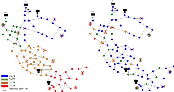
The case study used to evaluate the model is shown in Figure 2, which is the modification from an example of the EPANET software, namely the Net3 network. The network has 2 reservoirs, 3 tanks, 92 nodes, 117 pipes and 2 pumps. The demands in the network are classified into four different demand patterns. Two configurations of the demand patterns are considered in this study. In Figure 2.a, the demands are divided based on the topographic information, which results in a geographically distributed demand network. In Figure 2.b, the demands are categorized, as an example, based on the magnitudes of the base demands: DMF1 for nodes with base demands less than 10 L/s, DMF2 for nodes with base demands from 10 L/s to 20 L/s, DMF3 for nodes with base demands from 20 L/s to 30 L/s and DMF4 for nodes with base demands larger than 30 L/s. In this case, the network has non-geographically distributed demand patterns.

It is assumed that there are 12 pressure measurement sites randomly located within the network. The inputs for the near real-time demand estimation model are, therefore, the pressures at these locations, the tank levels of the three tanks and the pump statuses at each hour time step.

Figure 2. Case study network - (a) Geographically distributed demand patterns, (b) Non- geographically distributed demand patterns

It is also assumed that the default patterns, which are calibrated based on historical water used data, of four demand groups are known. In order to evaluate the estimation results of the PF model, measurement data sets are synthetically generated for a period of 48 hours as follows: (1) a random deviation N(0, 0.15) sampled from a normal distribution is added to each default demand pattern to create an “actual” demand pattern; (2) EPANET is run to generate two sets of nodal pressures at measured locations, corresponding with two configurations of the demand patterns; (3) a random

error is added to each nodal pressure. Three scenarios of random errors are considered: ∆meas = 0 (perfect measurement), ∆meas = ±0.5 m and ∆meas = ±1.0 m.

Table 1 shows the parameters applied in the PF model. The estimation results for the geographically distributed demand pattern network as well as the non-geographically distributed demand pattern network associated with different level of measurement errors are summarised in the following sections.

Table 1. Particle filter model parameters

PF model parameters Values Auto regression coefficient 0.7

Variance of noise 0.16 Number of particles 100,000

3.1

Perfect measurements

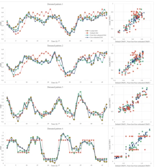
The left hand side plots of Figure 3 give the default DMFs, the actual DMFs and the estimated DMFs for the geographically distributed and non-geographically distributed patterns over 48 hours. The right hand side plots of Figure 3 display the scattergrams of the default DMFs as well as the estimated DMFs versus their actual values.

Without considering measurement errors, the PF model provides good estimates of the DMFs for these networks. By assimilating real-time pressure information into the estimation process, the default demand patterns are adjusted, approaching the actual patterns. This adjustment can be observed in Table 2, via the values of the coefficients of determination (R2) and mean absolute error (MAE) of each demand pattern. The default DMFs show an average correlation to the actual DMFs with (R2) ranging from 0.709 to 0.814, while the estimated DMFs for both geographically distributed and non-geographically distributed demand patterns are strongly correlated to the actual ones with all R2 values being close to unity. It is also seen that the PF model gives better estimates for the network with geographically distributed demand patterns than the network with non-geographically distributed demand patterns, as the R2 values are closer to unity and the MAE values are smaller.

Table 2. Comparison of the estimation derived from the PF model when the measurements are considered error free (R2 – Coefficient of determination, MAE – Mean absolute error)

DMFs Default DMFs Geo. distributed DMFs Non-Geo. distributed DMFs

R2 _{MAE R}2 _{MAE R}2 _MAE

DMF1 0.709 0.097 0.956 0.041 0.895 0.049 DMF2 0.703 0.101 0.975 0.023 0.868 0.053 DMF3 0.840 0.175 0.949 0.102 0.909 0.144 DMF4 0.814 0.259 0.983 0.081 0.940 0.159

3.2

Measurement errors

Two levels of measurement errors including ∆meas = ±0.5 m and ∆meas = ±1.0 m for all measurements are considered for the second test of the PF model. The accuracy of the estimates, presented by the same assessment criteria (R2 and MAE), as shown in Table 3 and Table 4.

Table 3. Comparison of the estimation from the PF model when

∆

DMFs Geographically distributed DMFs Non-Geo. distributed DMFs

R2 _{MAE R}2 _MAE

DMF1 0.864 0.071 0.812 0.062

DMF2 0.954 0.032 0.818 0.064

DMF3 0.934 0.120 0.905 0.141

DMF4 0.977 0.089 0.946 0.153

It is observed that with relative small measurement errors (

∆

provide reasonable estimates of the DMFs in both networks. The MEA values are smaller and R2 values are larger for both networks (compared to the default DMFs in Table 2), which means that the PF model has shifted the default DMFs closer to the actual DMFs. Similar to the previous test, the estimation results of the PF model for the geographically distributed demand pattern network are more accurate than for the non-geographically distributed demand pattern network, especially for DMF2 and DMF4.

The values in Table 4, on the other hand, show that with large measurement errors (

∆

the PF model cannot provide good estimates of the DMFs. For the geographically distributed demand pattern network, the estimated DMF1 has very weak correlation with the actual DMF1. The estimates of DMF2 and DMF3 show an accuracy similar to the default patterns. Better estimation results can only be achieved in DMF4, where the demand group is connected to the others by a single pipe and the pressure in this region is mainly dependent on the pressure in Tank 2.

For the non-geographically distributed demand pattern network, the estimated DMF1, DMF2 and DMF3 are even more inaccurate. The estimated DMF4, which is associated with nodes with largest base demands in the network, is slightly improved because this demand group dominates the other demand groups. Due to large base demands, small changes in this pattern can cause a large change in the demand at these nodes, which subsequently results in a large change in the pressure at measured locations.

Table 4. Comparison of the estimation from the PF model when

∆

DMFs Geographically distributed DMFs Non-Geo. distributed DMFs

R2 _{MAE R}2 _MAE

DMF1 0.527 0.113 0.458 0.136

DMF2 0.778 0.092 0.577 0.140

DMF3 0.847 0.220 0.809 0.202

DMF4 0.941 0.145 0.869 0.235

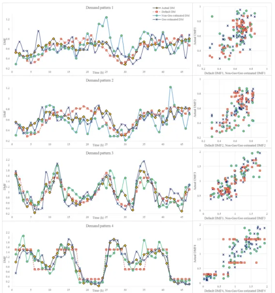
The estimated DMFs derived from the PF model that considers a measurement error of

∆

this extended period. In this case, the default demand patterns would be a better input for a hydraulic model and would provide a more accurate representation of the real network behaviour.

4

CONCLUSIONS

The work in this paper has evaluated the performance of the PF model proposed by [2] for the near real-time estimation of water demand multipliers. Two types of networks have been studied: a geographically distributed demand pattern network and a non-geographically distributed demand pattern network. Different level of measurement errors have also been examined. Results show that the PF model can be used for relatively large networks with multiple demand patterns. Well estimated DMFs can be obtained if the measurement errors are relatively small. The model cannot provide good estimates if large errors are contained in the measurement data. In addition, the results also show that the model performs better with the geographically distributed demand pattern network than with the non-geographically distributed demand pattern network for all scenarios.

References

[1] N.C. Do, A.R. Simpson, J.W. Deuerlein & O. Piller, 'Calibration of Water Demand Multipliers in Water Distribution Systems Using Genetic Algorithms', Journal of Water Resources Planning and Management, p. 04016044, 2016.

[2] N.C. Do, A.R. Simpson, J.W. Deuerlein & O. Piller, 'A particle filter - based model for online estimation of demand multipliers in water distribution systems under uncertainty', Journal of Water Resources Planning and Management, accepted on 18 May 2017

[3] D. Kang & K. Lansey, 'Real-time demand estimation and confidence limit analysis for water distribution systems', Journal of Hydraulic Engineering, vol. 135, no. 10, pp. 825-837, 2009.

[4] F. Odan, L.R. Reis & Z. Kapelan, ‘Real-Time Multiobjective Optimization of Operation of Water Supply Systems’, Journal of Water Resources Planning and Management, vol. 141, no. 9, 10.1061/(ASCE)WR.1943-5452.0000515, 04015011, 2015.

[5] G. Sanz, R. Pérez, Z. Kapelan & D. Savic, ‘Leak detection and localization through demand components calibration’ Journal of Water Resources Planning and Management, 142(2), p.04015057, 2015.

[6] J.E. van Zyl, O. Piller & Y. le Gat, 'Sizing municipal storage tanks based on reliability criteria', Journal of Water Resources Planning and Management, vol. 134, no. 6, pp. 548-555, 2008.

[7] C. Beal & R. Stewart, 'Identifying Residential Water End Uses Underpinning Peak Day and Peak Hour Demand', Journal of Water Resources Planning and Management, vol. 140, no. 7, p. 04014008, 2014.

[8] L.A. Rossman, 'EPANET 2: users manual', US Environmental Protection Agency (EPA), USA, 2000.

[9] J.D. Hol, T.B. Schon & F. Gustafsson, 'On resampling algorithms for particle filters', Nonlinear Statistical Signal Processing Workshop, 2006 IEEE, IEEE, pp. 79-82, 2006.