AN EFFICIENT NO-REFERENCE METRIC FOR PERCEIVED BLUR

HAL Id: hal-00606007

https://hal.archives-ouvertes.fr/hal-00606007

Submitted on 2 Nov 2011

HAL is a multi-disciplinary open access

archive for the deposit and dissemination of

sci-entific research documents, whether they are

pub-lished or not. The documents may come from

teaching and research institutions in France or

abroad, or from public or private research centers.

L’archive ouverte pluridisciplinaire HAL, est

destinée au dépôt et à la diffusion de documents

scientifiques de niveau recherche, publiés ou non,

émanant des établissements d’enseignement et de

recherche français ou étrangers, des laboratoires

publics ou privés.

AN EFFICIENT NO-REFERENCE METRIC FOR

PERCEIVED BLUR

Hantao Liu, Junle Wang, Judith Redi, Patrick Le Callet, Heynderickx Ingrid

To cite this version:

Hantao Liu, Junle Wang, Judith Redi, Patrick Le Callet, Heynderickx Ingrid. AN EFFICIENT

NO-REFERENCE METRIC FOR PERCEIVED BLUR. 2011 3rd European Workshop on Visual

Information Processing (EUVIP), Jul 2011, Paris, France. pp.6. �hal-00606007�

AN EFFICIENT NO-REFERENCE METRIC FOR PERCEIVED BLUR

Hantao Liu

, Junle Wang

, Judith Redi

, Patrick Le Callet

and Ingrid Heynderickx

1

Department of Mediamatics, Delft University of Technology, Delft, The Netherlands

2

IRCCyN, Ecole Polytechnique de l'Universite de Nantes, Nantes, France

3

Group Visual Experiences, Philips Research Laboratories, Eindhoven, The Netherlands

ABSTRACT

This paper presents an efficient no-reference metric that quantifies perceived image quality induced by blur. Instead of explicitly simulating the human visual perception of blur, it calculates the local edge blur in a cost-effective way, and applies an adaptive neural network to empirically learn the highly nonlinear relationship between the local values and the overall image quality. Evaluation of the proposed metric using the LIVE blur database shows its high prediction accuracy at a largely reduced computational cost. To further validate the performance of the blur metric on its robustness against different image content, two additional quality perception experiments were conducted: one with highly textured natural images and one with images with an intentionally blurred background1. Experimental results demonstrate that the proposed blur metric is promising for real-world applications both in terms of computational efficiency and practical reliability.

Index Terms♥ Image quality assessment, objective

metric, perceived blur, edge, neural network

1. INTRODUCTION

Blur is one of the important attributes in image quality assessment [1]. Developing an objective metric, which automatically quantifies perceived blur, is of fundamental importance to a broad range of applications, such as the optimization of auto-focus systems, super-resolution techniques, and sharpness enhancement in displays. In many real-world applications, there is no access to the distortion-free reference image, thus these objective metrics need to be of the no-reference (NR) type. This implies that the assessment of blur is based on the distorted image only. Achieving a NR metric that reliably predicts the extent to which humans perceive blur, while being computationally efficient for real-time applications, is still challenging.

1

The subjective data and the implementation of the metric are available on the web-site: http://mmi.tudelft.nl/iqlab/index.html

Existing blur metrics are formulated either in the spatial domain or in the frequency transform domain. The metrics implemented in the transform domain (see e.g. [2]-[4]) usually involve a rather complex calculation of energy falloff in the DCT or wavelet transform domain. Moreover, some metrics require the access to the encoding parameters, which are, however, not always available in practical applications. A blur metric defined in the spatial domain generally relies on measuring the spread of edges in an image (see e.g. [5]-[7]). Perhaps, the simplest and most well-known edge-based blur metric is the one proposed in [5], which estimates the overall blur annoyance by simply calculating the averaged local edge width. It, however, shows limitations in predicting perceived blur, partly due to its lack of including aspects of the human visual system (HVS). To improve the reliability of a blur metric, researchers investigated explicit simulation of the way human beings perceive blur (see e.g. [6] and [7]). The metric in [6] refines the calculation of local blur by adjusting the edge detection and by adding an existing model for masking by the HVS. In [7], a more dedicated human perception model of JNB (Just Noticeable Blur) is integrated in a blur metric. Both metrics in [6] and [7] are claimed to be more consistent with subjective data, but they heavily rely on the sophisticated and expensive modeling of the HVS. A known approach to avoid the explicit simulation of the assessment of overall quality is the use of a neural network (NN) (see e.g. [8]-[10]). However, these approaches usually start from the selection of active features from a set of generic image characteristics, a process that is rather ad hoc and computationally extensive. In this paper, we propose a novel blur metric that combines the advantages of two approaches, i.e. the dedicated calculation of the local edge blur in the spatial domain, and the use of a NN to yield overall quality resulting from blur. The proposed metric is validated using the LIVE blur database, and is compared against alternatives existing in literature. Two additional subjective experiments for perceived quality induced by blur were conducted: one with highly textured, natural images and one with images having an intentionally blurred background. The resulting subjective data are highly

beneficial to evaluate the performance of blur metrics for larger variations in image content.

2. PROPOSED NR BLUR METRIC

The schematic overview of the proposed NR blur metric is shown in Figure 1. It consists of two components: first, extraction of the features effectively describing the local edge blur, and second, the use of an adaptive NN to learn the highly nonlinear relationship between the dedicated features and the overall quality ratings. After appropriate training with subjective data, the NN yields a model that at run-time calculates the perceived quality from the extracted features without considerable computational effort. Details of the implementation are explained below.

Fig. 1. Schematic overview of the proposed NR blur metric. 2.1. Feature Extraction

2.1.1. Local Edge Blur Estimation

Measuring the smoothing or smearing effect on strong edges has been proved to be an effective approach to approximate perceived blur in an image [5]-[7]. To detect strong edges literature offers a wide variety of techniques (e.g. [14] and its references). As already mentioned in [19], an advanced edge detection method would be beneficial for improving the robustness of local edge blur estimation, but at the expense of computational efficiency. In this paper, we use a straightforward Sobel edge detector resulting in a gradient image, mainly to limit the metric’s complexity. The location of the strong edges is then extracted applying a threshold to this gradient image (as such removing noise and insignificant edges). The threshold value is automatically set depending on the image content (e.g. using the mean of the squared gradient magnitude over the image).

Instead of calculating the distance between the start and end position of an edge (as described in [5]), we propose to locally define edge blur in the gradient domain as the gradient energy of the edge related to its surrounding content within a limited extent. When the luminance channel of an image of M×N (height×width) pixels is denoted as I(i, j) for iΓ[1, M], jΓ[1, N], the local edge blur Lblur-h along the horizontal direction is quantified as:

Lblur-h(i, j)=

å

(i, j) Γ {strong edges}(1)

where Gh(i, j) indicates the gradient map along the horizontal direction, and is computed as:

Gh(i, j)= I(i,j+1)-I(i,j) jÎ[1,N-1] (2)

and n determines the size of the template used to describe the local content. The size is determined as a balance between collecting sufficient information of the local content and avoiding noise from content too far away (i.e.

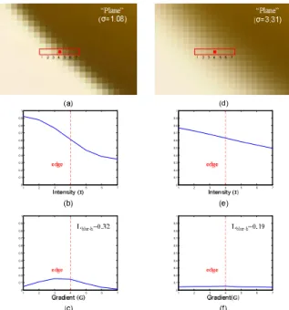
n=3 in our experiments). Lblur-v, i.e. the local blur in the vertical direction, can be calculated similarly. The lower the value of Lblur-h and Lblur-v, the larger the distortion of the blur artifact is. Figure 2 explains the reasoning behind the proposed approach of using gradient energy to detect blur.

1 2 3 4 5 6 7 0 0.1 0.2 0.3 0.4 0.5 0.6 0.7 0.8 0.9 1 1 2 3 4 5 6 7 0 0.1 0.2 0.3 0.4 0.5 0.6 0.7 0.8 0.9 1 1 2 3 4 5 6 7 0 0.1 0.2 0.3 0.4 0.5 0.6 0.7 0.8 0.9 1 1 2 3 4 5 6 7 0 0.1 0.2 0.3 0.4 0.5 0.6 0.7 0.8 0.9 1

Fig. 2. Illustration of the calculation of local edge blur: (a) image

patch extracted from an image (i.e. “img86” of the LIVE blur database [15]) [the red dot indicates the location of the detected edge at (252, 101) in this image, and the template indicates the area in which the local blur is calculated for this edge], (b) the intensity profile over the pixels within the template of (a), (c) the gradient profile of (b), (d) the same image patch of a blurred version of image (a) i.e. “img139” of the LIVE database, (e) the intensity profile over the pixels within the template of (d), and (f) the gradient profile of (e).

Direct application of all extracted values of local edge blur as input to a NN is problematic, since the dimensionality of these values is in general too large and varies with image content, and as such inappropriate for the network in terms of training. First, high dimensionality of the input might introduce noise and redundancies, with the consequent risk of over-fitting. Second, the architecture of a NN has to be fixed prior the training, therefore a varying number of input is not allowed. In this paper, the statistical description of an image feature as proposed in [8] and [9] is adopted. It unifies the local blur values to a single vector using percentiles. Having computed the local values fi (i=1, … , NF, and NF is the total number of the local values) per image (i.e. Lblur calculated in both the horizontal and vertical direction on the detected edges), these values are sorted in ascending order of magnitude. The outline of the obtained distribution is then expressed in a global descriptor f by taking 11 of its percentiles ナ:

f={j_a;aÎ{0,10,20,30,40,50,60,70,80,90,100}}; úû ù êë é ₊ = 2 1 100a ja F N (3)

2.2. NR Quality Estimator Based on a Neural Network

Computational intelligence tools are known for their ability of dealing with highly complex modeling problem. In particular, theory proves that feed-forward neural networks embedding a sigmoidal nonlinearity can support arbitrary mappings [11]. In this paper, a feed-forward NN is employed to map the extracted feature vector describing the local edge blur into the associated rating of perceived quality. The implementation of this NN is already described in more detail in [8] and [9], and is only briefly repeated here.

A Circular Back Propagation (CBP) [12] network improves the conventional MultiLayer Perceptron (MLP) [13] paradigm by adding one more input value, which is the sum of the squared values of all the network inputs (see Figure 1). The quadratic term boosts the network’s representation ability without affecting the fruitful properties of an MLP structure.

The CBP architecture can be described as follows. For an input stimulus vector x={x1, … , xni}, the input layer connects the ni values to each of the nh neurons of a hidden layer. The j-th hidden neuron performs a nonlinear transformation of a weighted combination of the input values with coefficients (“weights”) wj,i (j=1, … , nh, and i=1, … , ni): ) ( 1 2 1 , 1 , 0 ,

å

å

where sigm(z)=(1+e-z)-1, wj,0 is a bias term, and aj is the neuron activation. The output layer provides the actual network response, y: ) ( 1 0

å

For a fixed architecture (i.e. nh is fixed empirically before the training, see [8] and [9]), the CBP network is trained to optimize the desired input-output mapping, minimizing a cost function which measures the mean squared error between the actual NN output and the expected reference output (i.e. the MOS) for a sample of training patterns.

3. PSYCHOVISUAL EXPERIMENTS

A sub-set of the LIVE database comprising Gaussian blurred images [15] has been extensively adopted to validate blur metrics. It contains twenty-nine high-quality colored source images that reflect diversity in image content. These source images are filtered using a circular-symmetric 2-D Gaussian kernel of standard deviation σ B, ranging from 0.42 to 15 pixels, which results in a set of 174 stimuli (including the source images). Since the LIVE database is limited in its amount of demanding images, we performed two additional quality perception experiments. For example, the LIVE database includes only two source images with distinct foreground objects against a rather homogeneous background, as illustrated in Figure 3. In addition, also the amount of highly textured images is limited in the LIVE database. Evaluating how well a blur metric is able to handle these more demanding images is valuable for various applications; in particular the evaluation of images with a distinct foreground object against a homogeneous background is relevant for professional photography. Hence, we propose to extend the evaluation of the robustness of blur metrics with more image content. To that end, we make the data of two additional experiments of perceived quality resulting from blur available: one experiment used natural images of highly textured content, and the second experiment used images with an intentionally blurred background.

Fig. 3. The two source images of the LIVE database [15] that

3.1. Highly Textured Images (HTI) Database

The first quality perception experiment was conducted at the A University. A set of 12 images with highly textured content, as illustrated in Figure 4, was used as source material. These source images were high-quality colored images of size 512×768 (height×width) pixels. They were blurred in the same way and with the same range of σ B as the images of the LIVE database. Since each source image was blurred at five different levels, we obtained a test database of 72 stimuli (including the source images). The stimuli were displayed on a Dell 24” LCD screen with a native resolution of 1920×1200 pixels. The experiment was conducted in a standard office environment and the viewing distance was approximately 70cm. Eighteen participants, being ten males and eight females, were recruited for the experiment. A single-stimulus (SS) image quality assessment methodology as described in [16] was used and the raw data were processed according to the method described in [14] to produce the mean opinion scores (MOS).

Fig. 4. Source images of the HTI database.

3.2. Database of the Intentionally Blurred Background Images (IBBI)

Fig. 5. Source images of the IBBI database.

The second quality perception experiment was conducted at the B University. A new set of 12 images having an intentionally blurred background, as illustrated in Figure 5,

was extracted from [17]. Also these images were colored, and they had a size of 321×481 (height×width) pixels. Their background was blurred showing an obvious effect of depth of field. Since also these 12 images were blurred with the same five levels of σ B, again a database of 72 stimuli was obtained. The stimuli were displayed on a Samsung 22” LCD screen with a resolution of 1680×1050. They were viewed in a darkened room at a distance of approximately 60cm. Eighteen subjects participated in this experiment. They were requested to assess the overall image quality using again the single-stimulus (SS) image quality assessment methodology as described in [16]. The raw data were processed towards the MOS in the same way as for the HTI database.

4. EVALUATION OF METRIC PERFORMANCE 4.1. Performance Evaluation of the Proposed Metric

To fairly evaluate the performance of the proposed NR blur metric, a K-fold cross-validation method [8] was adopted. It randomized the statistical design problem by repeatedly splitting the available data into a training set and a test set. The source images were divided into several (i.e. six for the LIVE database and four for the HTI/IBBI database) groups. The entire procedure included six different trials for the LIVE database and four for the HTI/IBBI database. For each trial (hereafter referred to as “run”) five/three (for the LIVE database and HTI/IBBI databases, respectively) groups of source images were used for training and the remaining one group of source images was used for testing. In our experiments, for each image, a vector containing eleven percentiles of the distribution of the local blur features was calculated as the input to the NN, which was equipped with three hidden neurons (i.e. nh =3).

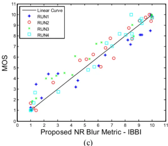
The performance of our metric was quantified by the Pearson linear correlation coefficient (CC) and the root mean squared error (RMSE) (note: the scores are normalized to the scale [1, 10] before the calculation of the RMSE) between the subjective quality ratings (the MOS) and the predictions of the metric. Figure 6 illustrates the scatter plot of the MOS versus the quality prediction for the test images of the LIVE, HTI and IBBI databases, respectively. The corresponding CC and RMSE values are listed in Table 1. Both the figure and the table show that our proposed metric consistently results in a high prediction performance for all runs of each database. Since the performance for the more demanding images of the HTI/IBBI databases is largely comparable to the performance for the images of the LIVE database, our proposed NR blur metric demonstrate its robustness against a large variation in image content.

Table 1. Performance evaluation of the proposed NR blur metric

(based on the K-fold cross-validation method used in [8]). LIVE, HTI and IBBI refer to each of the databases. CC and RMSE refer to the Pearson linear correlation coefficient and the

root-mean-square error, respectively.

LIVE HTI IBBI

CC RMSE CC RMSE CC RMSE

RUN1 0.9468 1.0256 0.9896 0.4732 0.9596 1.0460 RUN2 0.9597 0.8147 0.9822 0.5723 0.9743 0.6862 RUN3 0.9554 1.2555 0.9825 0.5749 0.9780 0.9872 RUN4 0.9804 0.5234 0.9819 0.6489 0.9812 0.6229 RUN5 0.9515 0.6766 RUN6 0.9857 0.4536 MEAN 0.9633 0.8216 0.9840 0.5673 0.9733 0.8356

To make an even more critical evaluation of our metric, we trained it with one database, and tested it with the other two databases (i.e. referred to as cross database evaluation). Table 2 lists the corresponding CC values. Our metric indeed demonstrates its promising performance; e.g. when training it with the limited HTI/IBBI databases, it still yields a high CC value (over 0.9) on the LIVE database.

Table 2. Cross database evaluation of the proposed NR blur

metric (based on training with one database and testing on the other two).

Training Set Test Set

LIVE (174) HTI (72) IBBI (72)

LIVE (174) 0.9770 0.9652

HTI (72) 0.9394 0.9758

IBBI (72) 0.9028 0.9602

4.2. Comparison to Alternative Metrics

In the image quality community, researchers are accustomed to compare the performance of their metric to that of alternatives available in literature. This allows these researchers to better understand the strengths and weaknesses of all metrics. For practical reasons the comparison of our proposed metric to alternative NR blur metrics is limited to the metric described in [5] (hereafter referred to as NRPB) and the one described in [7] (hereafter referred to as JNBM). Table 3 lists the performance of these metrics in terms of Pearson correlation coefficient.

In order to check whether the numerical differences in metric performance are statistically significant or not, a variance-based hypothesis test was conducted. It is based on the residuals between the quality predicted by the blur metric and the MOS (hereafter referred to as BM-MOS residuals) [18]. The results of the statistical significance tests are presented in Table 4, whereas the results of the Gaussianity tests are given in Table 5. It should, however, be noted that statistical significance testing is not straightforward, and the conclusions drawn from it largely depend e.g. on the number of sample points, on the selection of the confidence criterion, and on the assumption of Gaussianity of the residuals.

The NRPB metric is simple, but its performance is limited as compared to our proposed metric, as can be seen from Table 3. The lower performance might be a direct consequence of the fact that the NRPB simply maps the averaged local blur to the quality scores with a nonlinear transformation only. Our proposed metric clearly outperforms NRPB, yet without introducing additional computational cost. Our metric also exhibits a better performance than the JNBM metric. In addition, since the latter contains sophisticated modeling of the HVS, our proposed metric has its advantages in terms of computational complexity.

5. CONCLUSIONS

In this paper, we present an efficient NR metric for the assessment of perceived image quality induced by blur. It calculates local edge blur in a computationally inexpensive way, and leaves the simulation of the HVS for the perceived overall quality to an adaptive neural network. The proposed metric is validated with the sub-set of blur images of the LIVE database and with the content of two newly created databases of demanding images. The performance of our metric is compared to state-of-the-art alternatives in the literature and shows to be highly consistent with subjective data at a largely reduced computational complexity. Combined with its practical reliability and computational efficiency, our metric is a good alternative for real-time implementation.

Table 3. Performance comparison in terms of CC between our

proposed metric and state-of-the-art NR blur metrics (a nonlinear regression (see [18]) is applied to NRPB [5] and JNBM [7]).

NR Blur Metric LIVE (174) HTI (72) IBBI (72) NRPB [5] 0.8959 0.9413 0.9136 JNBM [7] 0.8425 0.9490 0.9238 Proposed 0.9633 0.9840 0.9733

Table 4. Matrix representing the results of the statistical

significance tests based on BM-MOS residuals. Each entry in the table is a codeword consisting of three symbols. The position of the symbol in the codeword represents the databases (from left to

right): LIVE, HTI and IBBI. Each symbol gives the result of the hypothesis test: “1” means that the blur metric for the row is statistically significantly better that the blur metric for the column,

“0” means that it is statistically significantly worse, and “-” means that there is no difference.

NRPB [5] JNBM [7] Proposed

NRPB [5] --- 0-- 0--

JNBM [7] 1-- --- 000

Proposed 1-- 111 ---

Table 5. Gaussianity of the BM-MOS residuals: “1” means that

the residuals can be assumed to have a normal distribution since the Kurtosis lies between 2 and 4.

LIVE (174) HTI (72) IBBI (72)

JNBM [7] 0 0 1

Proposed 0 1 1

6. REFERENCES

[1] Z. Wang and A. C. Bovik, Modern Image Quality Assessment, Morgan & Claypool Publishers, Mar, 2006.

[2] X. Marichal, W. Ma and H. Zhang, “Blur determination in the compressed domain using DCT information,” in Proc. IEEE ICIP, pp. 386-390, 1999. [3] J. Caviedes and F. Oberti, “A new sharpness metric

based on local kurtosis, edge and energy information,”

Signal Processing: Image Communication, 18(1), pp.

147-161, 2004.

[4] R. Hassen, Z. Wang and M. Salama, “No-reference image sharpness assessment based on local phase coherence measurement,” in Proc. IEEE ICASSP, pp. 2434-2437, 2010.

[5] P. Marziliano, F. Dufaux, S. Winkler and T. Ebrahimi, “A no-reference perceptual blur metric,” in Proc. IEEE

ICIP, pp. 57-60, 2002.

[6] L. Liang, J. Chen, S. Ma, D. Zhao, W. Gao, “A no-reference perceptual blur metric using histogram of gradient profile sharpness,” in Proc. IEEE ICIP, pp. 4369-4372, 2009.

[7] R. Ferzli and L. J. Karam, “A no-reference objective image sharpness metric based on the notion of just noticeable blur (JNB),” IEEE Trans. on Image

Processing, vol. 18, pp. 717–728, 2009.

[8] P. Gastaldo and R. Zunino, “Neural networks for the no-reference assessment of perceived quality,” Journal

of. Electronic Imaging, 14 (3), 033004, 2005.

[9] J. Redi, P. Gastaldo, I. Heynderickx and R. Zunino, “Color Distribution Information for the Reduced-Reference Assessment of Perceived Image Quality,”

IEEE Trans. on Circuits and Systems for Video Technology, 2010.

[10] R. V. Babu, S. Suresh and A. Perkis, “No-reference JPEG-image quality assessment using GAP-RBF,” Signal Processing, vol. 87, no.6, pp.1493-1503, 2007. [11] K. Hornik, M. Stinchcombe and H. White,

“Multilayered feedforward networks are universal approximators,” Neural Networks, vol.2, no.5, pp. 359-66, 1989.

[12] S. Ridella, S. Rovetta, and R. Zunino, “Circular back-propagation networks for classification,” IEEE

Transactions on Neural Networks, vol. 8, no. 1, pp.

84-97, 1997.

[13] D. E. Rumelhart and J. L. McClelland, Parallel distributed processing. MIT Press, Cambridge, MA, 1986.

[14] H. Liu, N. Klomp and I. Heynderickx, “A No-Reference Metric for Perceived Ringing Artifacts in

Images,” IEEE Trans. on Circuits and Systems for

Video Technology, vol. 20, pp. 529-539, 2010.

[15] H. R. Sheikh, Z. Wang, L. Cormack and A. C. Bovik, "LIVE Image Quality Assessment Database Release 2," http://live.ece.utexas.edu/research/quality

[16] J. Redi, H. Liu, H. Alers, R. Zunino and I. Heynderickx, "Comparing subjective image quality measurement methods for the creation of public databases", in Proc.

IS&T/SPIE Electronic Imaging, vol. 7529, 2010.

[17] D. Martin, C. Fowlkes, D. Tal and J. Malik, “A Database of Human Segmented Natural Images and its Application to Evaluating Segmentation Algorithms and Measuring Ecological Statistics,” in Proc. IEEE

ICCV, vol. 2, pp. 416-423, 2001.

[18] VQEG, “Final report from the video quality experts group on the validation of objective models of video quality assessment, phase II,” http://www.vqeg.org [19] H. Liu and I. Heynderickx, “Issues in the design of a

no-reference metric for perceived blur,” in Proc. SPIE-IS&T Electronic Imaging, Image Quality and System Performance VIII, 2011. 0 1 2 3 4 5 6 7 8 9 10 11 0 1 2 3 4 5 6 7 8 9 10 11

Proposed NR Blur Metric - LIVE

MO S Linear Curve RUN1 RUN2 RUN3 RUN4 RUN5 RUN6 (a) 0 1 2 3 4 5 6 7 8 9 10 11 0 1 2 3 4 5 6 7 8 9 10 11

Proposed NR Blur Metric - HTI

MO S Linear Curve RUN1 RUN2 RUN3 RUN4 (b)

0 1 2 3 4 5 6 7 8 9 10 11 0 1 2 3 4 5 6 7 8 9 10 11

Proposed NR Blur Metric - IBBI

MO S Linear Curve RUN1 RUN2 RUN3 RUN4 (c)

Fig. 6. Performance of the proposed NR blur metric: (a) (b) and (c)

are the scatter plot of the MOS versus the proposed metric of all runs for the LIVE, HTI and IBBI databases, respectively.