HAL Id: hal-00877643
https://hal.archives-ouvertes.fr/hal-00877643v2
Submitted on 12 May 2014
HAL is a multi-disciplinary open access
archive for the deposit and dissemination of
sci-entific research documents, whether they are
pub-lished or not. The documents may come from
teaching and research institutions in France or
abroad, or from public or private research centers.
L’archive ouverte pluridisciplinaire HAL, est
destinée au dépôt et à la diffusion de documents
scientifiques de niveau recherche, publiés ou non,
émanant des établissements d’enseignement et de
recherche français ou étrangers, des laboratoires
publics ou privés.
Applying the Adaptive Hybrid Flow-Shop Scheduling
Method to Schedule a 3GPP LTE Physical Layer
Algorithm onto Many-Core Digital Signal Processors
Julien Heulot, Jani Boutellier, Maxime Pelcat, Jean François Nezan,
Slaheddine Aridhi
To cite this version:
Julien Heulot, Jani Boutellier, Maxime Pelcat, Jean François Nezan, Slaheddine Aridhi. Applying
the Adaptive Hybrid Flow-Shop Scheduling Method to Schedule a 3GPP LTE Physical Layer
Algo-rithm onto Many-Core Digital Signal Processors. NASA/ESA Conference on Adaptive Hardware and
Systems (AHS-2013), Jun 2013, Turino, Italy. pp.Pages 123 - 129. �hal-00877643v2�
Applying the Adaptive Hybrid Flow-Shop
Scheduling Method to Schedule a 3GPP LTE
Physical Layer Algorithm onto Many-Core Digital
Signal Processors
Julien Heulot
∗, Jani Boutellier
§, Maxime Pelcat
∗, Jean-Franc¸ois Nezan
∗, Slaheddine Aridhi
∗∗∗IETR, INSA Rennes, CNRS UMR 6164, UEB
Rennes, France
email: jheulot, mpelcat, [email protected]
§University of Oulu
FI-90014 University of Oulu, Finland email: [email protected]
∗∗Texas Instruments France
Villeneuve Loubet, France email: [email protected]
Abstract—Currently, Multicore Digital Signal Processor (DSP) platforms are commonly used in telecommunications baseband processing. In the next few years, high performance DSPs are likely to combine many more DSP cores for signal processing with some General-Purpose Processor (GPP) cores for application control. As the number of cores increases in new DSP platform designs, scheduling of applications is becoming a complex opera-tion. Meanwhile, the variability of the scheduled applications also tends to increase as applications become more sophisticated. Such variations require runtime adaptivity of application scheduling.
This paper extends the previous work on adaptive scheduling by using the Hybrid Flow-Shop (HFS) scheduling method, which enables the device architecture to be modeled as a pipeline of Processing Elements (PEs) with multiple alternate PEs for each pipeline stage. HFS scheduling is applied to the scheduling of 3rd Generation Partnership Project (3GPP) Long Term Evolution (LTE) telecommunication standard Uplink Physical Layer data processing (PUSCH).
The experiments, conducted on an ARM Cortex-A9 GPP, show that an HFS scheduling algorithm has an overhead that increases very slowly with the number of PEs. This makes the method suitable for executing the adaptive scheduling in less than 1 ms for the 501 actors of a LTE PUSCH dataflow description executed on a 256-core architecture.
I. INTRODUCTION
Today, multicore Digital Signal Processor (DSP) platforms are commonly used in signal processing, such as baseband processing in telecommunications and multimedia applica-tions. Although the use of multi-core processors is widespread, the system-level complexity of the platforms causes myriad problems which still remain unsolved.
Computationally, the most powerful multi-core DSP plat-forms (Texas Instruments TMS320C6678 and Freescale P4080 for instance) currently comprise up to 8 DSP cores. The next generation DSP TMS320TCI6636 from Texas Instruments will combine a 4-core ARM Cortex-A15 General-Purpose Processor (GPP) and 8 c66x DSP cores. Combining GPP cores dedicated to control-oriented operations and application
This work was supported by the ANR COMPA project
scheduling and DSP cores dedicated to signal processing may become a typical internal architecture for computationally powerful DSP processors. Moreover, if the current trend to integrate increasingly more cores in processors continues [1], many-core DSP processors, comprising a few GPP cores and many powerful DSP cores, made possible by higher integration density may prevail in a few years over other DSP processors. Two major issues in multiprocessing are a) the nature of the interconnect topology [2] and b) the scheduling and synchronization of computations. In fact, these two issues can not be separated from each other, as the interconnect dictates the nature of the scheduling approach. In this paper, the term Processing Element (PE) is used to refer to either a DSP core or a dedicated co-processor.
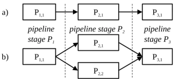
Pipelined interconnects and their scheduling are of high relevance in DSP and multimedia applications [3, Page 124]. An example of pipelined interconnects can be seen in Figure 1. Figure 1 a) depicts a classical pipeline with three stages, each consisting of one PE. Figure 1 b) depicts a slightly more complex pipeline where the second stage has two PEs (#2 and #3) that can process data concurrently.
In the Hybrid Flow-Shop (HFS) scheduling method [4], used in the proposed methodology, the target architecture is modeled as in Figure 1 b). For multi-core architectures that allow bidirectional (isotropic) inter-processor communication, the HFS scheduling method restricts communication to fixed, unidirectional links. This dramatically reduces the complexity of adaptive scheduling and makes the overhead of scheduling up to 256 PEs manageable (Section V).
It has been shown previously [5] that the highly dynamic nature of the Uplink Physical Layer data processing (PUSCH) decoding algorithm executed in 3rd Generation Partnership Project (3GPP) Long Term Evolution (LTE) base stations does not allow the use of static multiprocessor schedules; fast adaptive scheduling is mandatory. [5] used a list scheduling method to schedule 3GPP LTE PUSCH decoding on a multi-core DSP. This method is not applicable to many-multi-core adaptive scheduling (with hundreds of PEs), as 1/9 of the computation is dedicated to scheduling which involves 8 PEs.
P1,1 P2,1 P3,1 P1,1 P2,2 P3,1 P2,1 a) b) pipeline
stage P1 pipeline stage P2 pipelinestage P3
Fig. 1. Three stage pipelines with a) one PE per stage, b) one or more PEs per stage.
In this paper, we propose a method based on HFS sched-uling to adaptively schedule the 3GPP LTE PUSCH algorithm onto many-core architectures. We show that HFS scheduling can be applied to schedule applications on pipelines of proces-sors that have parallel PEs at arbitrary stages. As an application example we show how the 3GPP LTE telecommunication stan-dard PUSCH can be modeled as an HFS scheduling problem and that the simplifying assumptions of HFS scheduling enable the fast computation of an efficient many-core schedule.
The adaptive scheduling of classical pipelines (as in Fig-ure 1 a)) has been previously studied [6], [7], whereas the more complex hybrid case containing stages with parallel PEs (as in Figure 1 b)) is still largely unexplored in the context of signal processing.
This paper is formulated as follows: Section II discusses work related to the topics discussed in this publication; Sec-tion III presents the PUSCH applicaSec-tion; SecSec-tion IV shows how the PUSCH application can be modeled as an HFS scheduling problem; Section V shows experimental results on scheduling of 3GPP LTE PUSCH and Section VI concludes the paper.
II. RELATED WORK
The use and scheduling of PE pipelines in signal processing has been previously studied. In [6], MPEG-4 macroblock decoding was modeled as a classical flow-shop scheduling problem and [7] extended the study to consider various in-termediate buffers between the pipeline stages.
The scheduling of the 3GPP LTE PUSCH decoding pro-cess has previously been discussed in the work of Pelcat et al. [5]. In this work it was shown that static scheduling of PUSCH is unfeasible and that an adaptive scheduler is necessary. The applied list scheduling method provided very high-quality schedules, but the context of [5] was different to this work, as the assumed platform was isotropic and the resulting communications were not restricted in their direction. The review article of Ruiz et al. [4] gives an overview of available methods for solving HFS scheduling problems. However, only a small minority of these are applicable to the problem at hand, as task graphs that depict DSP algorithms (such as PUSCH) generally have precedence constraints. Fi-nally, as our context is the adaptive scheduling of pipelined PEs, none of the presented solutions in [4] are suitable due to their complexity or restricted applicability.
[3, Page 129] lists several approaches for compile-time mapping of DSP algorithms to pipelined multiprocessors. Due
to the dynamic nature of the LTE PUSCH decoding process, these approaches are not applicable.
III. 3GPP LTE PUSCH PROCESSING
The 3GPP telecommunication standards, GSM and 3G, are used by billions of people over the world. The 3GPP LTE telecommunication standard improves the peak data rates in downlink to more than 100Mbit/s and peak uplink data rates to over 50Mbit/s. Theoretically, up to one hundred simultaneous users can share this available bandwidth.
The high performance is acquired by advanced tech-niques of Multiple Input Multiple Output (MIMO), Orthogonal Frequency-Division Multiple Access (OFDMA) in the down-link and Single-Carrier Frequency-Division Multiple Access (SC-FDMA) in the uplink processing [8]. These techniques must be implemented both in the physical layer of LTE base stations (which are also known as eNodeB) and in the User Equipment (UE) such as cell phones.
The use of these complex techniques in variable condi-tions requires high adaptivity from the processing platform. To maintain the real-time, power-efficiency and versatility requirements of the LTE physical layer processing, multi-core DSPs with hardware coprocessors are the platform of choice. However, the scheduling and synchronization of the physical layer processing on a multiprocessor platform is a considerable challenge.
A. PUSCH Processing Stages
Rem. CP Freq. Shift FFT Rem. CP Freq. Shift FFT Rem. CP Freq. Shift FFT
SC-FDMA and multiple antennas decoding (static) Subcarrier demapping RF/
ADC
IDFT
Constellation demapping and bit processing (dynamic) RF/ ADCRF/ ADCRF/ ADC Rem. CP Freq. Shift FFT
Constellation demapping Bit process Turbo dec CRC check
Channel estimation
+ Equalization
Fig. 2. PUSCH high level processing chain: static and dynamic parts.
The physical layer decoding operation [8] can be roughly divided in two parts as shown in Figure 2 :
1) The static part: The Cyclic Prefix (CP) is removed,
the symbols are converted into frequency domain by a Fast Fourier Transform (FFT) and equalized using channel estimation on received reference signals. The subcarriers are then reordered and, finally, an Inverse Discrete Fourier Transform (IDFT) reconverts the data back into the time domain per user basis.
2) The dynamic part: constellation demapping and bit
processing. For these operations, the parameters are highly variable during runtime (number of connected UEs, number of allocated Code Blocks (CBs), mod-ulation order, and so on). The multi-core scheduling of this dynamic part must be adaptive [5]. A de-tailed graph description of this part is shown in Section III-B.
The first (static) part of processing can be represented as a Synchronous Dataflow graph (SDF [3]) and represents a high level of parallelism. Consequently, a design tool can efficiently parallelize these operations at compile time. However, for the second (dynamic) part, the multi-core scheduling needs to be adapted to the varying parameters.
The LTE uplink physical layer bandwidth may vary be-tween 1.4 MHz and 20 MHz. In the most complex case of 20MHz, the base station (eNodeB) Medium Access Control (MAC) scheduler can assign resources to about 20 dynamically allocated users and 30 Voice over LTE users (VoLTE) semi-persistently. This translates to 50 variable size CBs, associated with these 50 UEs , being transmitted every millisecond. Given the number of UEs and their CB sizes, the dynamic part of PUSCH needs also to be rescheduled onto the multi-core architecture every millisecond. The next section explains the model used to represent the dynamic part of the PUSCH algorithm.
B. Dataflow Description of the LTE PUSCH Decoding Dy-namic Part
In order to schedule the decoding of one LTE PUSCH subframe every millisecond, a parameterized model of the algorithm is required. Dataflow has proven to be an efficient representation for signal processing applications [3].
The vertices of dataflow graphs are known as actors. Actors consume data tokens on their input edges, process the data and produce result tokens on their output edges. Data between actors are exchanged exclusively via edges, representing First In, First Out data queues (FIFOs). An actor fires (executes) as long as there is data to consume on its input edges.
The graph model used to represent the dynamic part of LTE PUSCH is the Parameterized Cyclo-Static Directed Acyclic
Graph (PCSDAG)[5]. Rather than a new model, it is a subset of the Cyclo Static Dataflow Model (CSDF [9]) parameterized obeying the semantics of [10]. It has two main advantages:
• As a subset of CSDF, it can compactly model an
algorithm with complex production or consumption patterns. This is the case of the current PUSCH algorithm because the size of the CB assigned to each user varies greatly, both in time and between users.
• The simplifications enable a fast computation of
ac-tor repetitions gathered in a repetition vecac-tor. A new graph called single rate Directed Acyclic Graph (srDAG) can then be generated, duplicating actors by their repetition factors.
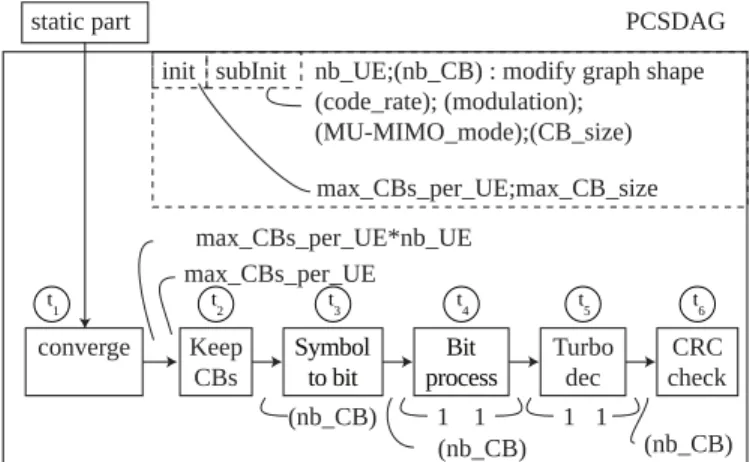
Both data token production and consumption of each PCSDAG edge is set by the MAC scheduler based on UE time and frequency scheduling. Figure 3 shows a simplified view of the LTE PUSCH PCSDAG description. The shape of the graph depends on the following parameters:
• the current number of UEs: nb U E,
• A pattern of parameters giving the number of CBs
allocated in each 1ms subframe to each UE: nb CB = {CBs U E1,CBs U E2,CBs U E3...}. This pattern has a maximum length of 50.
Other parameters influence the Deterministic Actor Exe-cution Time (DAET) of each actor, i.e. the time needed to execute each LTE PUSCH actor on each processing element. Pattern parameters are shown in parentheses in Figure 3. The
init phase is executed at system initialization while subinit
phase is executed for each 1 ms subframe.
static part converge PCSDAG max_CBs_per_UE*nb_UE max_CBs_per_UE max_CBs_per_UE;max_CB_size init subInit Keep CBs Symbolto bit
nb_UE;(nb_CB) : modify graph shape (code_rate); (modulation);
(MU-MIMO_mode);(CB_size)
Bit
process Turbodec checkCRC (nb_CB) 1 1 1 1 (nb_CB) (nb_CB) t2 t3 t4 t1 t5 t6
Fig. 3. PCSDAG description of the LTE PUSCH dynamic part with parameters recomputed every 1 ms.
Ignoring the effect of PCSDAG graph parameters on DAETs, the number of possible graph configurations is shown to be over 190 million [5]. Taking into account the DAET modifications, the number of possible graphs is even higher; thus is not suitable to precompute and store schedules.
In the next section we show how the PCSDAG formulation can be transformed into a HFS scheduling problem, and we present a PE pipeline-targeting scheduling approach that is sufficiently fast given the constraint of the 1 ms time frame for scheduling the PUSCH algorithm. Dataflow actors are con-verted into flow-shop tasks. This transformation is illustrated
in Figure 3 where actors are converted into tasks ti.
IV. PROPOSED SOLUTION
The origins of the flow-shop scheduling problem formu-lation are in factory production lines where multiple pro-duction machines work in parallel and products move from one machine to another as they are assembled. The flow-shop scheduling problem involves the processing of N jobs on M machines. In the classical flow-shop formulation each job consists of a set of operations, so that each operation has to be processed on exactly one machine. Due to our context, we shall name the machines as PEs and operations as tasks.
In the classical flow-shop formulation it is assumed that tasks have deterministic execution timings. This constraint is respected in our study case as we suppose each actor to have a DAET. Each job must pass through the PEs in a prescribed order, although it is possible for individual tasks to skip PEs. We assume that the optimization objective of the flow-shop problem is makespan minimization instead of other possible scheduling objectives. This is compatible with LTE constraints. The HFS scheduling method changes the setting by allow-ing several PEs to process one type of task [4]. Figure 4 a)
time ta,1 P1,1 P2,1 P2,2 P3,1 ta,2 ta,3 tb,1 tb,2 tb,3 tc,1 tc,2 tc,3 time ta,1 P1,1 P2,1 P3,1 ta,2 ta,3 tb,1 tb,2 tb,3 tc,1 tc,2 tc,3 t1 a) b) c) t2 t3
Job J Job instance Ja ta,1 ta,2 ta,3
tb,1 tb,2 tb,3
Job instance Jb
tc,1 tc,2 tc,3
Job instance Jc
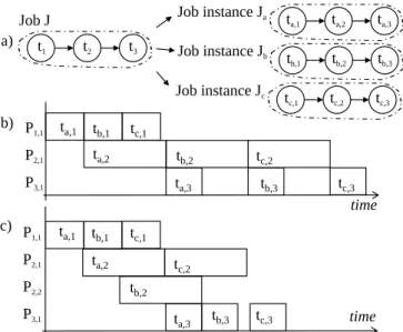
Fig. 4. a) 3 instances of one job J consisting of three tasks. b) Instances of J scheduled on architecture shown in Figure 1 a). c) Instances of J scheduled on architecture shown in Figure 1 b).
This little task graph represents a flow-shop job. The job exists
in three instances: Ja, Jb and Jc. Figure 4 b) shows the Gantt
chart (schedule) when the job instances Ja, Jb and Jc have
been scheduled onto the pipelined multiprocessor architecture shown in Figure 1 a). Respectively, Figure 4 c) shows the same jobs scheduled on the pipelined architecture of Figure 1
b), where PE2 and PE3 are both capable of executing task t2.
Figure 4 highlights the common situation where one kind
of task (t2, in this case) is computationally more demanding
than other tasks in the application and thus forms a bottleneck in the processing pipeline. The classical flow-shop formulation can not represent cases where a long-latency task is distributed to more than one PE, whereas in HFS scheduling method this is no problem. In LTE PUSCH the variance in task execution times is high: on a programmable DSP the individual PCSDAG actors have execution time differences of one order of magnitude [5].
In this work, some common flow-shop assumptions are used: jobs are processed in every stage in the same order; each task is processed at most by one PE at each pipeline stage; all jobs are available simultaneously before the scheduling starts; tasks pre-emption is not allowed. We also assume that there is enough buffer space between pipeline stages to hold the data during inter-stage communication and that communication times are included to task execution times.
Next, in SubSection IV-A we show how the LTE PUSCH decoding process can be formulated as an HFS scheduling problem and SubSection IV-B describes how schedules are computed out of HFS job sequences.
A. Flow-shop jobs from PCSDAG
The PCSDAG graph is a simple linear graph that is capable of capturing all the variability of the PUSCH algorithm within its parameters. To enable HFS scheduling, the PUSCH PCSDAG graph must be transformed to HFS jobs.
P3,1 P4,2 P5,1 P4,1 P2,2 P2,1 a) b) c) static part P3 P4 P5 P1 t1,1 t4,1 t4,2 t5,3 t3,3 t6,5 t6,4 t5,2 t4,4 t3,2 t2,2 t1,5 t1,4 t2,1 t3,1 t4,3 t5,1 t6,3 t6,2 t1,3 J1 J2 J3 J5 J6 t1 t2 t3 t4 t5 t6 x1 x3 x3 x6 x6 x3 t1,2 t6,1 J4 P2 P1,1
Fig. 5. a) PCSDAG graph b) Transformation to flow-shop jobs c) Mapping to 7 PEs.
The HFS scheduling method requires that every job has only one kind of task for each pipeline stage. In practice, this means that the pipeline mapping of PCSDAG actors affects the transformation from PCSDAG to HFS jobs; the mapping of actors to pipeline stages is the first step in the transformation. For general many-core platforms that have a full, isotropic interconnection network between PEs, applying HFS sched-uling implies that only a subset of the full interconnect needs to be used. Similarly, the PEs that are assigned to computations must be grouped as different pipeline stages.
In the PUSCH algorithm model there are some actors that have very short execution times and which execute only infrequently. As an extension of the base HFS scheduling method, the infrequent actors are mapped to pipeline stages that also execute computationally more burdening actors.
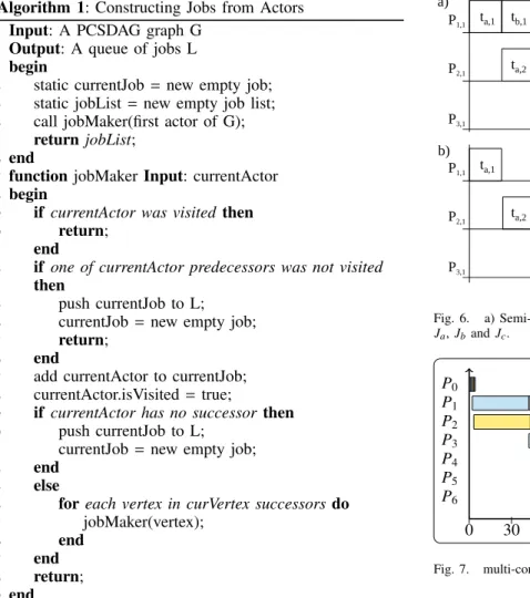
After the assignment of actors to pipeline stages, jobs can be extracted from the PCSDAG graph. The PCSDAG graph has a basis repetition vector that expresses how many times each PCSDAG actor is to be executed. As described in [5], the PCSDAG graph is transformed into a srDAG graph in which each vertex represents one HFS task instance. Figure 5 shows the transformation from a) PCSDAG to b) srDAG and finally to jobs, considering the 5-stage pipeline with 7 PEs in c).
In Figure 5 b), individual job instances are delimited by dashed borders. The algorithm used to create jobs from the srDAG graph is shown in Algorithm 1.
It is important to notice that the HFS jobs generated from the PCSDAG are not independent, as the case commonly is in the HFS scenario [4]. Looking at Figure 5, it must be kept in mind that the causality relationships between the srDAG actors still hold for the HFS jobs. Practically this means that the scheduling order of jobs is restricted somewhat.
Algorithm 1: Constructing Jobs from Actors Input: A PCSDAG graph G
Output: A queue of jobs L begin
1
static currentJob = new empty job; 2
static jobList = new empty job list; 3
call jobMaker(first actor of G); 4
return jobList; 5
end 6
function jobMaker Input: currentActor 7
begin 8
if currentActor was visited then 9
return; 10
end 11
if one of currentActor predecessors was not visited 12
then
push currentJob to L; 13
currentJob = new empty job; 14
return; 15
end 16
add currentActor to currentJob; 17
currentActor.isVisited = true; 18
if currentActor has no successor then 19
push currentJob to L; 20
currentJob = new empty job; 21
end 22
else 23
for each vertex in curVertex successors do 24 jobMaker(vertex); 25 end 26 end 27 return; 28 end 29 B. HFS scheduling
After the set of jobs, Ji,i ∈ [1,N], has been defined
and has been mapped to pipeline stages Pj,j ∈ [1,M], the
actual HFS scheduling can be conducted. In classical flow-shop the scheduling consists of two phases: 1) job ordering and 2) timetabling [6]. In HFS scheduling method, one more phase is added, which makes the sequence 1) job ordering, 2) assignment and 3) timetabling.
The purpose of job ordering is to place the jobs, Ji,i ∈
[1,N], to a sequence with the aim of minimizing the makespan
of the schedule. Job ordering for HFS scheduling has been studied extensively [4], but generally the ordering strategies are very time-consuming and not appropriate for runtime computations. For small job sets, there are simple job ordering heuristics [11], but as the number of jobs increases, the computation time of simple heuristics grows as well.
After job ordering has been conducted, the assignment
phase selects the actual processing element Pj,k out of the set
of PEs in stage Pj,k,k ∈ [1,Mj] to which task tm has been
assigned. In this work, earliest start assignment was used: at each step, the chosen PE grants the earliest start of the current task.
Timetabling defines when a specific task ti,m job J is allowed to start on a pre-defined pipeline stage j [11]. In
P1,1 ta,1 tb,1 tb,2 tb,3 tc,2 tc,1 time P2,1 P3,1 ta,2 ta,3 tc,3 P1,1 ta,1 tb,1 tb,2 tb,3 tc,2 tc,1 time P2,1 P3,1 ta,2 ta,3 tc,3 b) a)
Fig. 6. a) Semi-active and b) No-wait timetabling for the same set of jobs Ja, Jband Jc. 0 30 60 90 120 150 180 210 kcycles P6 P5 P4 P3 P2 P1 P0
Fig. 7. multi-core HFS scheduling of the example in Figure 5.
semi-activetimetabling, each task ti,mis started when both the previous task on the same PE has finished and the previous
task of the same job ti,m−1 has finished. In no-wait timetabling
each task (ti,m) within one job J is started immediately after
the previous task (ti,m−1) of the same job has finished. Figure 6
shows the difference of semi-active timetabling and no-wait timetabling in Gantt-charts.
Figure 7 shows the multi-core HFS scheduling of the example in Figure 5. The pipeline shape of the schedule is already visible for this small number of actors.
V. EXPERIMENTAL RESULTS
The trend of computationally efficient DSPs in the next few years is likely to consist of combining GPP cores for control and scheduling with many DSP cores for signal processing. In this context, experimental results will focus on the com-parison between list scheduling and HFS scheduling. Results have been acquired by scheduling a dataflow description of LTE PUSCH decoding for a many-core DSP on an ARM Cortex-A9 GPP processor. Experiments study the evolution of simulated makespan and adaptive scheduling time when PE count increases.
The timetabling approach used was semi-active. No-wait timetabling was also trialled, and produced almost identical makespans as semi-active timetabling. In the classical flow-shop situation no-wait timetabling has the additional benefit of
minimizing the buffer space requirements between PEs [11]. However, for HFS scheduling with jobs that have precedence constraints, the opposite is true. For this reason, no-wait timetabling was excluded from the present experiments.
A. Experiment Assumptions and Setup
Accordingly to Section III-B, the PUSCH algorithm com-prises of two variable parameters. The first is the number of UEs and the second is the number of Resource Blocks (RBs) allocated to each UE. For the LTE 20 MHz system, the total number of RBs available is 100. In the presented results, the number of UEs is set to 50, so the number of RBs per UE will vary between 1 and 3, giving a total of 100 RBs for all users. Because of the high number of users and the small resource block allocation per user, there will be just one CB per UE. This scenario results in a total of 50 CBs and illustrates one of the worst LTE PUSCH scheduling cases.
The hardware platform contains a dual-core ARM Cortex-A9 processor with a clock frequency of up to 1 GHz. The experimental adaptive scheduler is written in C++ and runs as a Linux mono-threaded task on the ARM processor. The embedded Cycle Counter (CCNT) provides accurate cycle measurements.
In order to compare schedules, tasks need to have known durations. Timing measurements used in this paper are based on a Texas Instrument c64x+ DSP. These timings do not limit the study, as the paper goal is to compare scheduling algorithms rather than publishing absolute schedule timings. Communication times between PEs are assumed to be part of the task timings. The simulated platform is thus a homo-geneous many-core platform with cores equivalent to c64x+ DSPs.
Two metrics are used to compare adaptive scheduling heuristics:
Makespan: The time difference between the start and the end of a given application graph execution. This is also known as latency.
Scheduling Overhead: The time necessary on the target platform to compute the adaptive scheduling algorithm, from acquiring PUSCH parameters to actor timetabling. As this time is not dedicated to signal processing, its minimization is necessary.
B. Results
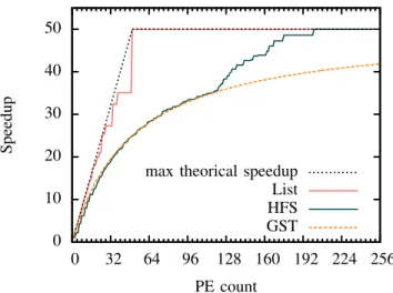
Results on makespan (Figure 8) compare both list and HFS scheduling algorithms to Greedy Scheduling Theorem (GST) algorithm [12]. GST curve gives an idea of the speedup that can be obtained with greedy scheduling, no actor timing knowledge and a fully-connected isotropic architecture with infinite communication rates [13].
In the test case, the algorithm critical path limits possible speedup to about 50 times. We see that list scheduling produces better speedup than HFS scheduling. List scheduling reaches critical path length limitation as soon as 50 PEs are available. On average, the makespan generated by HFS scheduling is 31% longer than that generated by list scheduling. The limi-tation of HFS scheduling in terms of makespan is due to its
0 10 20 30 40 50 0 32 64 96 128 160 192 224 256 Speedup PE count max theorical speedup
List HFS GST
Fig. 8. Makespan vs. # of PEs
0 500000 1e+06 1.5e+06 2e+06 2.5e+06 3e+06 3.5e+06 0 32 64 96 128 160 192 224 256 Cycles PE count HFS List
Fig. 9. Scheduling overhead vs. # of PEs
reduced mapping choices, as all PEs must communicate to a restricted list of PEs in a single direction.
The main advantage of HFS method is that its scheduling overhead (Figure 9) is increasing very slowly with the number of PEs, making the HFS method a good solution for many-core adaptive scheduling. This is not the case for a list scheduler whose scheduling overhead increases significantly with the number of PEs. In Figure 9, it may be seen that the HFS scheduler is faster once 17 PEs (or more) are available on the architecture. For fewer than 17 PEs, the time needed to construct HFS jobs makes HFS scheduling more costly than list scheduling.
If we look at Figure 10, we can see that the HFS scheduling overhead is divided into srDAG and job transformations that do not depend on the number of PEs and mapping and scheduling that do depend on the number of PEs.
We may conclude from our experiments that the HFS method has a very low scheduling overhead compared to the optimized list scheduling method when for higher PE count.
0 500000 1e+06 1.5e+06 2e+06 2.5e+06 3e+06 3.5e+06 8 128 256 8 128 256 Cycles PE count Job tranfo. HFS Map. HFS Sched. srDag tranfo. List Sched. List HFS
Fig. 10. Scheduling cost decomposition
HFS scheduling presupposes pipelined PEs and orientates inter-PE communications, simplifying PE assignment when compared to the general isotropic and fully-connected archi-tecture case. It also groups computing tasks into linear jobs, simplifying task scheduling while maintaining task precedence. For the case of 256 PEs and for all LTE PUSCH config-urations, the HFS method has a scheduling overhead under 1 Mcycles. This makes HFS scheduling suitable for real-time adaptive scheduling of studied LTE PUSCH worst case (comprising 501 actor instances) onto a 256-core architecture.
VI. CONCLUSION
In this paper, the HFS scheduling method was used to schedule the 3GPP LTE telecommunication standard PUSCH. The experiments demonstrated that a HFS scheduling algo-rithm on an embedded GPP has a very low computational scheduling overhead making the method suitable for adap-tive scheduling of the LTE PUSCH algorithm onto many-core architectures. Moreover, the speedup degradation of the generated many-core schedule is limited when compared to the makespan produced by the more costly list scheduling.
Besides producing low computational scheduling overhead, the HFS formulation additionally simplifies the inter-processor communication requirements on a many-core system. Whilst list scheduling requires a fully connected, bidirectional pro-cessor interconnection network, HFS scheduling thrives with a considerably smaller number of unidirectional inter-processor links.
We have extended the previous work of applying flow-shop scheduling to signal processing algorithms using HFS scheduling. HFS scheduling extends flow-shop scheduling by allowing each pipeline stage to have more than one PE, thus enabling pipeline balancing and makespan optimization. Experimental results show that HFS scheduling is a suitable method to schedule the worst case of the LTE PUSCH algo-rithm onto a 256-core architecture.
Directions for future work include evaluating the HFS scheduling on other applications to assess its capacity to schedule efficiently a wide range of applications.
References
[1] (2013, Jan.) Kalray MPPA. http://www.kalray.eu/products/mppa-manycore.
[2] L. J. Karam, I. AlKamal, A. Gatherer, G. A. Frantz, D. V. Anderson, and B. L. Evans, “Trends in Multicore DSP Platforms,” IEEE Signal Processing Magazine, vol. 26, 2009.
[3] S. Sriram and S. S. Bhattacharyya, Embedded Multiprocessors: Sched-uling and Synchronization, 2nd Edition. CRC Press, 2009.
[4] R. Ruiz and J. A. V´azquez-Rodr´ıguez, “The hybrid flow shop scheduling problem,” European Journal of Operational Research, vol. 205, no. 1, pp. 1–18, 2010. [Online]. Available: http://www.sciencedirect.com/science/article/pii/S0377221709006390 [5] M. Pelcat, J.-F. Nezan, and S. Aridhi, “Adaptive multicore scheduling
for the LTE uplink,” in NASA/ESA Conference on Adaptive Hardware and Systems, 2010, pp. 36–43.
[6] J. Boutellier, S. S. Bhattacharyya, and O. Silv´en, “Low-overhead run-time scheduling for fine-grained acceleration of signal processing systems,” in IEEE Workshop on Signal Processing Systems, 2007, pp. 457–462.
[7] J. Boutellier, “Quasi-static scheduling for fine-grained embedded mul-tiprocessing,” Ph.D. dissertation, University of Oulu, 2009.
[8] S. Sesia, I. Toufik, and M. Baker, LTE, The UMTS Long Term Evolution: From Theory to Practice. Wiley, 2009.
[9] G. Bilsen, M. Engels, R. Lauwereins, and J. A. Peperstraete, “Cyclo-static data flow,” in International Conference on Acoustics, Speech, and Signal Processing, 1995, pp. 3255–3258.
[10] B. Bhattacharya and S. Bhattacharyya, “Parameterized dataflow model-ing for DSP systems,” IEEE Transactions on Signal Processmodel-ing, vol. 49, no. 10, pp. 2408–2421, 2001.
[11] S. French, Sequencing and Scheduling: An Introduction to the Math-ematics of the Job-Shop. Chichester, UK: Ellis Horwood Limited, 1982.
[12] C. Leiserson, “A minicourse on dynamic multithreaded algorithms,” 2005.
[13] M. Pelcat, S. Aridhi, J. Piat, and J.-F. Nezan, Physical Layer Multi-Core Prototyping: A Dataflow-Based Approach for LTE eNodeB, 2013rd ed. Springer, Aug. 2012.