HAL Id: inria-00129309
https://hal.inria.fr/inria-00129309v5
Submitted on 16 Oct 2007
HAL is a multi-disciplinary open access
archive for the deposit and dissemination of
sci-entific research documents, whether they are
pub-L’archive ouverte pluridisciplinaire HAL, est
destinée au dépôt et à la diffusion de documents
scientifiques de niveau recherche, publiés ou non,
Dimitrios Diochnos, Ioannis Z. Emiris, Elias Tsigaridas
To cite this version:
Dimitrios Diochnos, Ioannis Z. Emiris, Elias Tsigaridas. On the complexity of real solving bivariate
systems. [Research Report] RR-6116, INRIA. 2007. �inria-00129309v5�
a p p o r t
d e r e c h e r c h e
Thème SYM
On the complexity of real solving bivariate systems
Dimitrios I. Diochnos — Ioannis Z. Emiris — Elias P. Tsigaridas
N° 6116
Dimitrios I. Diochnos
∗, Ioannis Z. Emiris
†, Elias P. Tsigaridas
‡ §Thème SYM — Systèmes symboliques Projet VEGAS
Rapport de recherche n° 6116 — June 2007 — 55 pages
Abstract: This paper is concerned with exact real solving of well-constrained, bivariate al-gebraic systems. The main problem is to isolate all common real roots in rational rectangles, and to determine their intersection multiplicities. We present three algorithms and analyze their asymptotic bit complexity, obtaining a bound of eOB(N14) for the purely
projection-based method, and eOB(N12) for two subresultant-based methods: we ignore polylogarithmic
factors, and N bounds the degree and the bitsize of the polynomials. The previous record bound was eOB(N16).
Our main tool is signed subresultant sequences, extended to several variables by the technique of binary segmentation. We exploit recent advances on the complexity of univari-ate root isolation, and extend them to multipoint evaluation, to sign evaluation of bivariunivari-ate polynomials over two algebraic numbers, and real root counting for polynomials over an extension field. Our algorithms apply to the problem of simultaneous inequalities; they also compute the topology of real plane algebraic curves in eOB(N12), whereas the previous
bound was eOB(N16).
All algorithms have been implemented in maple, in conjunction with numeric filtering. We compare them against fgb/rs and system solvers from synaps; we also consider maple libraries insulate and top, which compute curve topology. Our software is among the most robust, and its runtimes are comparable, or within a small constant factor, with respect to the C/C++ libraries.
Key-words: maple code, real solving, polynomial systems, real algebraic numbers, com-plexity
This work is partially supported by the european project ACS (Algorithms for Complex Shapes, IST FET Open 006413) and ARC ARCADIA (http://www.loria.fr/∼petitjea/Arcadia/)
∗Department of Informatics and Telecommunications National Kapodistrian University of Athens,
HEL-LAS
†Department of Informatics and Telecommunications National Kapodistrian University of Athens,
HEL-LAS
‡LORIA-INRIA Lorraine, Nancy, FRANCE
Résumé : On s’intéresse à la résolution exacte, dans les réels, de systèmes algébriques bien-contraints en deux variables. Le problème principal est d’isoler les racines communes en des rectangles rationaux, et de calculer leur multiplicités. Nous présentons trois algorithmes et nous analysons leur complexité asymptotique binaire, arrivant à une borne de eOB(N14) pour
la méthode de projection, et de eOB(N12) pour les deux méthodes basées sur le résultant:
ces bornes ignorent les facteurs poly-logarithmiques, où N borne le degré et la taille binaire des polynômes. La borne précedente était de eOB(N16).
Notre outil principal sont les séquences de sous-résultants, généralisées en plusieurs va-riables. Nous nous basons sur les avancés récentes sur la complexité d’isolation univariée, et nous généralisons ces résultats pour borner la complexité de l’ évaluation en plusieurs points, pour déterminer le signe de polynômes en deux variables, et pour compter le nombre de racines d’un polynôme en coefficients algébriques. Nos algorithmes s’appliquent au pro-blème d’inégalités simultanées; ils calculent aussi la topologie d’une courbe algébrique dans le plan en eOB(N12), tandis que la borne existante était de eOB(N16).
Nos algorithmes ont tous été implementés en Maple, avec filtrage numérique. Nous les comparons avec gbrs, des solveurs de synaps, ainsi que les programmes insulate et top en maple, qui calculent la topologie d’une courbe. Notre logiciel est parmi les plus robustes et ses temps de calculs sont comparables, ou plus lents d’un petit facteur constant, par rapport aux logiciels C/C++.
Mots-clés : code Maple, résolution dans les réels, systèmes algébriques, nombres algé-briques, complexité
1
Introduction
The problem of well-constrained polynomial system solving is fundamental. However, most of the algorithms treat the general case or consider solutions over an algebraically closed field. We focus on real solving of bivariate polynomials, in order to provide precise complex-ity bounds and study different algorithms in practice. We expect to obtain faster algorithms than in the general case. This is important in several applications ranging from nonlinear computational geometry to real quantifier elimination. We suppose relatively prime polyno-mials for simplicity, but this hypothesis is not restrictive. A question of independent interest is to compute the topology of a plane real algebraic curve.
Our algorithms isolate all common real roots inside non-overlapping rational rectangles, and output them as pairs of algebraic numbers; they also determine the intersection mul-tiplicity per root. In this paper, OB means bit complexity and eOB means that we are
ignoring polylogarithmic factors. We derive a bound of eOB(N12), whereas the previous
record bound was eOB(N14) [GVEK96], see also [BPM06], derived from the closely related
problem of computing the topology of real plane algebraic curves, where N bounds the de-gree and the bitsize of the input polynomials. This approach depends on Thom’s encoding. We choose the isolating interval representation, since it is more intuitive, it is used in appli-cations, and demonstrate that it supports as efficient algorithms as other representation. In [GVEK96] it is stated that “isolating intervals provide worst [sic] bounds”. Moreover, it is widely believed that isolating intervals do not produce good theoretical results. Our work suggests that isolating intervals should be re-evaluated.
Our main tool is signed subresultant sequences (closely related to Sturm-Habicht se-quences), extended to several variables by the technique of binary segmentation. We exploit the recent advances on univariate root isolation, which reduced complexity by 1-3 orders of magnitude to eOB(N6) [DSY05, ESY06, EMT07]. This brought complexity closer to
e
OB(N4), which is achieved by numerical methods [Pan02].
In [KSP05], 2 × 2 systems are solved and the multiplicities computed under the assump-tion that a generic shear has been obtained, based on [SF90]. In [Wol02], 2 × 2 systems of bounded degree were studied, obtained as projections of the arrangement of 3D quadrics. This algorithm is a precursor of ours, see also [ET05], except that matching and multiplicity computation was simpler. In [MP05], a subdivision algorithm is proposed, exploiting the properties of the Bernstein basis, with unknown bit complexity, and arithmetic complexity based on the characteristics of the graphs of the polynomials. For other approaches based on multivariate Sturm sequences the reader may refer to e.g. [Mil92, PRS93].
Determining the topology of a real algebraic plane curve is a closely related problem. The best bound is eOB(N14) [BPM06, GVEK96]. In [WS05] three projections are used; this is
implemented in insulate, with which we make several comparisons. Work in [Ker06] offers an efficient implementation of resultant-based methods. For an alternative using Gröbner bases see [CFPR06]. To the best of our knowledge the only result in topology determination using isolating intervals is [AM88], where a eOB(N30) bound is proved.
We establish a bound of eOB(N12) using the isolating interval representation. It seems
that the complexity in [GVEK96] could be improved to eOB(N10) using fast multiplication
algorithms, fast algorithms for computations of signed subresultant sequences and improved bounds for the bitsize of the integers appearing in computations. To put our bounds into perspective, note that the input is inOB(N3), and the bitsize of all output isolation points
for univariate solving is eOB(N2), and this is tight.
The main contributions of this paper are the following: Using the aggregate separation bound, we improve the complexity for computing the sign of a polynomial evaluated over all real roots of another (lem. 2.7). We establish a complexity bound for bivariate sign evaluation (th. 3.7), which helps us derive bounds for root counting in an extension field (lem. 5.1) and for the problem of simultaneous inequalities (cor. 5.4). We study the complexity of bivariate polynomial real solving, using three projection-based algorithms: a straightforward grid method (th. 4.1), a specialized RUR approach (th. 4.6), and an improvement of the latter using fast GCD (th. 4.7). Our best bound is eOB(N12); within this bound, we also compute
the root multiplicities. Computing the topology of a real plane algebraic curve is in eOB(N12)
(th. 5.6).
We implemented in maple a package for computations with real algebraic numbers and for implementing our algorithms. It is easy to use and integrates seminumerical filtering to speed up computation when the roots are well-separated. It guarantees exactness and completeness of results; moreover, the runtimes seem very encouraging. We illustrate it by experiments against well-established C/C++ libraries fgb/rs and synaps. We also examine maple libraries insulate and top, which compute curve topology. Our software is robust and effective; its runtime is within a small constant factor with respect to the fastest C/C++ library.
The next section presents basic results concerning real solving and operations on uni-variate polynomials. We extend the discussion to several variables, and focus on biuni-variate polynomials. The algorithms for bivariate solving and their analyses appear in sec. 4, fol-lowed by applications to real-root counting, simultaneous inequalities and the topology of curves. Our implementation and experiments appear in sec. 6.
2
Univariate polynomials
For f ∈ Z[y1, . . ., yk, x], dg(f ) denotes its total degree, while degx(f ) denotes its degree
w.r.t. x. L (f ) bounds the bitsize of the coefficients of f (including a bit for the sign). We assume lg (dg(f )) = O(L (f )). For a ∈ Q, L (a) is the maximum bitsize of numerator and denominator. Let M (τ ) denote the bit complexity of multiplying two integers of size τ , and M (d, τ ) the complexity of multiplying two univariate polynomials of degrees ≤ d and coefficient bitsize≤ τ . Using FFT, M (τ ) = eOB(τ ), M (d, τ ) = eOB(dτ ).
Let f, g ∈ Z[x], dg(f ) = p ≥ q = dg(g) and L (f ) , L (g) ≤ τ . We use rem (f, g) and quo (f, g) for the Euclidean remainder and quotient, respectively. The signed poly-nomial remainder sequence of f, g is R0 = f , R1 = g, R2 = − rem (f, g), . . . , Rk =
− rem (Rk−2, Rk−1), where rem (Rk−1, Rk) = 0. The quotient sequence contains Qi =
quo(Ri, Ri+1), i = 0 . . . k − 1, and the quotient boot is (Q0, . . . , Qk−1, Rk).
Here, we consider signed subresultant sequences, which contain polynomials similar to the polynomials in the signed polynomial remainder sequence; see [vzGL03] for a unified approach to subresultants. They achieve better bounds on the coefficient bitsize and have good specialization properties. In our implementation we use Sturm-Habicht sequences, see e.g. [GVLRR89]. By SR(f, g) we denote the signed subresultant sequence, by sr(f, g) the sequence of the principal subresultant coefficients, by SRQ(f, g) the corresponding quotient boot, and by SR(f, g; a) the evaluated sequence over a ∈ Q. If the polynomials are multi-variate, then these sequences are considered w.r.t. x, except if explicitly stated otherwise. Proposition 2.1 [LR01, LRSED00, Rei97] Assuming p ≥ q, SR(f, g) is computed in
e
OB(p2qτ) and L (SRj(f, g)) = O(pτ ). For any f, g, their quotient boot, any polynomial
in SR(f, g), their resultant, and their gcd are computed in eOB(pqτ ).
Proposition 2.2 [LR01, Rei97] Let p ≥ q. We can compute SR(f, g; a), where a ∈ Q ∪ {±∞} and L (a) = σ, in eOB(pqτ + q2σ+ p2σ). If f (a) is known, then the bound becomes
e
OB(pqτ + q2σ).
Proof. Let SRq+1 = f and SRq = g. For the moment we forget SRq+1. We may assume
that SRq−1is computed, since the cost of computing one element of SR is the same as that
of computing SRQ(f, g) (Pr. 2.1).
We follow Lickteig and Roy [LR01]. For two polynomials A, B of degree bounded by D and bit size bounded by L, we can compute SR(A, B)(a), where L (a) ≤ L, in eOB(M (D, L)).
In our case D = O(q) and L = O(pτ + qσ), thus the total costs is eOB(pqτ + q2σ).
It remains to compute the evaluation SRq+1(a) = f (a). This can be done using Horners’
scheme in eOB(p max{τ, pσ}). Thus, the whole procedure has complexity
e
OB(pqτ + q2σ+ p max{τ, pσ}),
where the term pτ is dominated by pqτ . 2 When q > p, SR(f, g) is f, g, −f, −(g mod (−f )) . . . , thus SR(f, g; a) starts with a sign variation irrespective of sign(g(a)). If only the sign variations are needed, there is no need to evaluate g, so prop. 2.2 yields eOB(pqτ + p2σ). Let L denote a list of real numbers. VAR(L)
denotes the number of (possibly modified, see e.g. [BPM06, GVLRR89]) sign variations. Corollary 2.3 For any f, g, VAR(SR(f, g; a)) is computed in eOB(pqτ + min{p, q}2σ),
pro-vided sign(f (a)) is known.
We choose to represent a real algebraic number α∈ Ralg by theisolating interval
repre-sentation. It includes a square-free polynomial which vanishes on α and a (rational) interval containing α and no other root.
Proposition 2.4 [DSY05, ESY06, EMT07] Let f ∈ Z[x] have degree p and bitsize τf.
We compute the isolating interval representation of its real roots and their multiplicities in eOB(p6+ p4τf2). The endpoints of the isolating intervals have bitsize O(p2+ p τf) and
L (fred) = O(p + τf).
The sign of the square-free part fred over the interval’s endpoints is known; moreover,
fred(a)fred(b) < 0.
Corollary 2.5 [BPM06, EMT07] Given a real algebraic number α ∼= (f, [a, b]), where L (a) = L (b) = O(pτf), and g ∈ Z[x], such that dg(g) = q, L (g) = τg, we compute
sign(g(α)) in bit complexity eOB(pq max{τf, τg} + p min{p, q}2τf).
Proof. Assume that α is not a common root of f and g in [a, b], then it is known that sign g(α) = [VAR(SR(f, g; a)) − VAR(SR(f, g; b))] sign(f′(α)).
Actually the previous relation holds in a more general context, when f dominates g, see [Yap00] for details. Notice that sign(f′(α)) = sign(f (b)) − sign(f (b)), which is known from
the real root isolation process.
The complexity of the operation is dominated by the computation of VAR(SR(f, g; a)) and VAR(SR(f, g; b)), i.e. we compute SRQ and evaluate it on a and b.
As explained above, there is no need to evaluate the polynomial of the biggest degree, i.e the first (and the second if p < q) of SR(f, g) over a and b. Thus the complexity is that of cor. 2.3, viz.
e
OB(pq max{τf, τg} + min{p, q}2p τf)
Thus the complexity of the operation is two times the complexity of the evaluation of the sequence over the endpoints of the isolating interval.
If α is a common root of f and g, or if f and g are not relative prime, then their gcd, which is the last non-zero polynomial in SR(f, g) is not a constant. Hence, we evaluate SR on a and b, we check if the last polynomial is not a constant and if it changes sign on a and b. If this is the case, then sign(g(α)) = 0. Otherwise we proceed as above. 2 Prop. 2.4 expresses the state-of-the-art in univariate root isolation. It relies on fast computation of polynomial sequences and the Davenport-Mahler bound, e.g. [Yap00]. The following lemma, derived from Davenport-Mahler’s bound, is crucial.
Lemma 2.6 (Aggregate separation) Given f ∈ Z[x], the sum of the bitsize of all isolat-ing points of the real roots of f is O(p2+ p τ
f).
Proof.[of lem. 2.6] Let there be r ≤ p real roots. The isolating point between two consec-utive real roots αj, αj+1 is of magnitude at most 12|αj− αj+1| := 12∆j. Thus their product
is 21r
Q
j∆j. Using the Davenport-Mahler bound, Qj∆j ≥ 2−O(p
2
+pτf) and we take
We present a new complexity bound on evaluating the sign of a polynomial g(x) over a set of algebraic numbers, which have the same defining polynomial, namely over all real roots of f (x). It suffices to evaluate SR(f, g) over all the isolating endpoints of f . The obvious technique, e.g. [EMT07], is to apply cor. 2.5 r times, where r is the number of real roots of f . But we can do better by applying lem. 2.6:
Lemma 2.7 Let τ = max{p, τf, τg}. Assume that we have isolated the r real roots of f and
we know the signs of f over the isolating endpoints. Then, we can compute the sign of g over all r roots of f in eOB(p2qτ).
Proof.[of lem. 2.7] Let sj be the bitsize of the j-th endpoint, where 0 ≤ j ≤ r. The
evalua-tion of SR(f, g) over this endpoint, by cor. 2.3, costs eOB(pqτ + min{p, q}2sj). To compute
the overall cost, we should sum over all the isolating points. The first summand is eOB(p2qτ).
By pr. 2.6, the second summand becomes eOB(min{p, q}2(p2+ pτf)) and is dominated. 2
3
Multivariate polynomials
We discuss multivariate polynomials, using binary segmentation [Rei97]. An alternative approach could be [Klo95]. Let f, g ∈ (Z[y1, . . . , yk])[x] with dgx(f ) = p ≥ q = dgx(g),
dgyi(f ) ≤ diand dgyi(g) ≤ di. Let d =
Qk
i=1di andL (f ) , L (g) ≤ τ . The yi-degree of every
polynomial in SR(f, g), is bounded by dgyi(res(f, g)) ≤ (p+q)di. Thus, the homomorphism
ψ: Z[y1, . . . , yk] → Z[y], where
y17→ y, y27→ y(p+q)d1, . . . , yk7→ y(p+q)
k−1d1···d k−1,
allows us to decode res(ψ(f ), ψ(g)) = ψ(res(f, g)) and obtain res(f, g). The same holds for every polynomial in SR(f, g). Now ψ(f ), ψ(g) ∈ (Z[y])[x] have y−degree ≤ (p + q)k−1d since, in the worst case, f or g hold a monomial such as yd1
1 yd 2 2 . . . y dk k . Thus, dgy(res(ψ(f ), ψ(g))) < (p + q)kd.
Proposition 3.1 [Rei97] We can compute SRQ(f, g), any polynomial in SR(f, g), and res(f, g) in eOB(q(p + q)k+1dτ).
Lemma 3.2 SR(f, g) is computed in eOB(q(p + q)k+2dτ).
Proof. Every polynomial in SR(f, g) has coefficients of magnitude bounded 2c(p+q)τ, for
a suitable constant c, assuming τ > lg(d). Consider the map χ : Z[y] 7→ Z, such that y 7→ 2⌈c(p+q)τ ⌉, and let φ = ψ ◦ χ : Z[y
1, y2. . . , yk] → Z. Then L (φ(f )) , L (φ(g)) ≤ c (p + q)kd τ.
Now apply pr. 2.1. 2
Theorem 3.3 We can evaluate SR(f, g) at x = α, where a ∈ Q ∪ {∞} and L (a) = σ, in e
Algorithm 1: sign_at(F, α, β)
Input: F ∈ Z[x, y], α ∼= (A, [a1, a2]), β ∼= (B, [b1, b2])
Output: sign(F (α, β)) compute SRQx(A, F ) 1
L1← SRx(A, F ; a1), V1← ∅ 2
foreach f ∈ L1do V1← add(V1, sign_at(f, β)) 3
L2← SRx(A, F ; a2), V2← ∅ 4
foreach f ∈ L2do V2← add(V2, sign_at(f, β)) 5
return (var(V1) − var(V2)) · sign(A′(α)) 6
Proof. Compute SRQ(f, g) in eOB(q(p+ q)k+1d τ) (prop. 3.1), then evaluate it over a, using
binary segmentation. For this we need to bound the bitsize of the resulting polynomials. The polynomials in SR(f, g) have total degree in y1, . . . , yk bounded by (p + q)Pki=1di
and coefficient bitsize bounded by (p + q)τ . With respect to x, the polynomials in SR(f, g) have degrees inO(p), so substitution x = a yields values of size eO(pσ). After the evalu-ation we obtain polynomials in Z[y1, . . . , yk] with coefficient bitsize bounded by max{(p +
q)τ, pσ} ≤ (p + q) max{τ, σ}.
Consider χ : Z[y] → Z, such that y 7→ 2⌈c(p+q) max{τ,σ}⌉, for a suitable constant c. Apply
the map φ = ψ ◦ χ to f, g. Now, L (φ(f )) , L (φ(g)) ≤ cd(p + q)kmax{τ, σ}. By prop. 2.2,
the evaluation costs eOB(q(p + q)k+1dmax{τ, σ}). 2
We obtain the following for f, g∈ (Z[y])[x], such that dgx(f ) = p, dgx(g) = q, dgy(f ), dgy(g) ≤
d.
Corollary 3.4 We compute SR(f, g) in eOB(pq(p + q)2dτ). For any polynomial SRj(f, g)
in SR(f, g), dgx(SRj(f, g)) = O(max{p, q}), dgy(SRj(f, g)) = O(max{p, q}d), and also
L (SRj(f, g)) = O(max{p, q}τ ).
Corollary 3.5 We compute SRQ(f, g), any polynomial in SR(f, g), and res(f, g) in eOB(pq max{p, q}dτ ).
Corollary 3.6 We compute SR(f, g ; a), where a ∈ Q∪{∞} and L (a) = σ, in eOB(pq max{p, q}d max{τ, σ}).
For the polynomials SRj(f, g ; a) ∈ Z[y], except for f, g, we have dgy(SRj(f, g ; a)) =
O((p + q)d) and L (SRj(f, g ; a)) = O(max{p, q}τ + min{p, q}σ).
We now reduce the computation of the sign of F ∈ Z[x, y] over (α, β) ∈ R2
alg to that
over several points in Q2. Let dg
x(F ) = dgy(F ) = n1, L (F ) = σ and α ∼= (A, [a1, a2]),
β ∼= (B, [b1, b2]), where A, B ∈ Z[X], dg(A) = dg(B) = n2,L (A) = L (B) = σ. We assume
n1≤ n2, which is relevant below. The algorithm is alg. 1, see [Sak89], and generalizes the
univariate case, e.g. [EMT07, Yap00]. For A, resp. B, we assume that we know their values on a1, a2, resp. b1, b2.
Proof. First, we compute SRQx(A, F ) so as to evaluate SR(A, F ) on the endpoints of α,
in eOB(n21n22σ) (cor. 3.5).
We compute SR(A, F ; a1). The first polynomial in the sequence is A, but we already
know its value on a1. This computation costs eOB(n21n32σ) by cor. 3.6 with q = n1, p = n2,
d= n1, τ = σ, and σ = n2σ, where the latter corresponds to the bitsize of the endpoints.
After the evaluation we obtain a list L1, which containsO(n1) polynomials, say f ∈ Z[y],
such that dg(f ) = O(n1n2). To bound the bitsize, notice that the polynomials in SR(f, g)
are of degrees O(n1) w.r.t. x and of bitsize O(n2σ). After we evaluate on a1, L (f ) =
O(n1n2σ).
For each f ∈ L1 we compute its sign over β and count the sign variations. We could
apply directly cor. 2.5, but we can do better. If dg(f ) ≥ n2 then SR(B, f ) = (B, f, −B,
g = − prem (f, −B) , . . . ). We start the evaluations at g: it is computed in eOB(n21n32σ)
(prop. 2.1), dg(g) = O(n2) and L (g) = O(n1n2σ). Thus, we evaluate SR(−B, g; a1) in
e
OB(n1n32σ), by cor. 2.5, with p = q = n2, τf = σ, τ = n1n2σ. If dg(f ) < n2the complexity
is dominated. Since we performO(n1) such evaluations, all of them cost eOB(n21n32σ).
We repeat for the other endpoint of α, subtract the sign variations, and multiply by sign(A′(α)), which is known from the process that isolated α. If the last sign in the two
sequences is alternating, then sign(F (α, β)) = 0. 2
4
Bivariate real solving
Let F, G∈ Z[x, y], dg(F ) = dg(G) = n and L (F ) = L (G) = σ. We assume relatively prime polynomials for simplicity but this hypothesis is not restrictive because it can be verified and if it does not hold, it can be imposed within the same asymptotic complexity. We study algorithms and their complexity for real solving the system F = G = 0. The main idea is to project the roots on the x and y axes, to compute the coordinates of the real solutions and somehow to match them. The difference between the algorithms is the way they match solutions.
4.1
The grid algorithm
Algorithm grid is straightforward, see also [ET05, Wol02]. We compute the x− and y−coordinates of the real solutions, as real roots of the resultants resx(F, G) and resy(F, G).
Then, we match them using the algorithm sign_at (th. 3.7) by testing all rectangles in this grid. The output is a list of pairs of real algebraic numbers represented in isolating interval representation. The algorithm also outputs rational axis-aligned rectangles, guaranteed to contain a single root of the system.
To the best of our knowledge, this is the first time that the algorithm’s complexity is studied. The disadvantage of the algorithm is that exact implementation of sign_at (alg. 1) is not efficient. However, its simplicity makes it attractive. The algorithm requires
Algorithm 2: grid(F, G) Input: F, G ∈ Z[x, y]
Output: The real solutions of F = G = 0 Rx← resy(F, G) 1 Lx, Mx← solve(Rx) 2 Ry← resx(F, G) 3 Ly, My← solve(Ry) 4 Q← ∅ 5 foreach α ∈ Lxdo 6 foreach β ∈ Ly do 7
if sign_at(F, α, β) = 0 ∧ sign_at(G, α, β) = 0 then Q ← add(Q, {α, β})
8
return Q
9
no genericity assumption on the input; we study a generic shear that brings the system to generic position in order to compute the multiplicities within the same complexity bound.
The algorithm allows the use of heuristics. In particular, we may exploit easily computed bounds on the number of roots, such as the Mixed Volume or count the roots with a given abscissa α by lem. 5.1.
Theorem 4.1 Isolating all real roots of system F = G = 0 using grid has complexity e
OB(n14+ n13σ), provided σ = O(n3).
Proof. First we compute the resultant of F and G w.r.t. y, i.e. Rx. The complexity is
e
OB(n4σ), using cor. 3.5. Notice that dg(Rx) = O(n2) and L (Rx) = O(n σ). We isolate its
real roots in eOB(n12+ n10σ2) (prop. 2.4) and store them in Lx. This complexity shall be
dominated. We do the same for the y axis and store the roots in Ly.
The representation of the real algebraic numbers contains the square-free part of Rx,
or Ry. In both cases the bitsize of the polynomial is O(n2+ n σ) [BPM06, EMT07]. The
isolating intervals have endpoints of sizeO(n4+ n3σ).
Let rx, resp. ry be the number of real roots of the corresponding resultants. Both are
bounded byO(n2). We form all possible pairs of real algebraic numbers from L
xand Lyand
check for every such pair if both F and G vanish, using sign_at (th. 3.7). Each evaluation costs eOB(n10+ n9σ) and we perform rxry= O(n4) of them. 2
We now examine the multiplicity of a root (α, β) of the system. Refer to [BK86, sec.II.6] for its definition as the exponent of factor (βx − αy) in the resultant of the (homogenized) polynomials, under certain assumptions.
The algorithm reduces to bivariate sign determination and does not require bivariate factorization. We shall use the resultant, since it allows for multiplicities to “project”. Pre-vious work includes [GVEK96, SF90, WS05]. The sum of multiplicities of all roots (α, βj)
equals the multiplicity of x = α in the respective resultant. It is possible to apply a shear transform to the coordinate frame so as to ensure that different roots project to different points on the x-axis.
4.1.1 Deterministic shear.
We determine an adequate (horizontal) shear such that
Rt(x) = resy(F (x + ty, y), G(x + ty, y)) , (1)
when t7→ t0 ∈ Z, has simple roots corresponding to the projections of the common roots
of the system F (x, y) = G(x, y) = 0 and the degree of the polynomials remains the same. Notice that this shear does not affect inherently multiple roots, which exist independently of the reference frame. Rred∈ (Z[t])[x] is the squarefree part of the resultant, as an element
of UFD (Z[t])[x], and its discriminant, with respect to x, is ∆ ∈ Z[t]. Then t0 must be such
that ∆(t0) 6= 0.
Example 4.2 Take the circle f = (x − 1)2+ y2− 1, and the double line g = y2 with two
double roots (0, 0), (2, 0). We shall project roots on the y-axis under the vertical shear: f(x, y + tx) = x2(1 + t2) + 2x(ty − 1) + y2, g(x, y + tx) = y2+ 2txy + (tx)2. Then, R(y) = y2[y2(t4+ 1) + 2t3y+ t2]. The square-free part is R
red(y) = y[y2(t4+ 1) +
2t3y+ t2] and ∆(t) = t6(t4+ 1)(3t4+ 4). Clearly, one must avoid the value t = 0, but any
other integer is valid.
Lemma 4.3 Computing t0 ∈ Z, such that the corresponding shear is sufficiently generic,
has complexity eOB(n10+ n9σ).
Proof. Suppose t0 is such that the degree does not change. It suffices to find, among n4
integer numbers, one that does not make ∆ vanish; note that all candidate values are of bitsizeO(log n).
We perform the substitution (x, y) 7→ (x+ty, y) to F and G and we compute the resultant w.r.t. y in eOB(n5σ), which is a polynomial in Z[t, x], of degree O(n2) and bitsize eO(dσ).
We consider this polynomial as univariate in x and we compute first its square-free part, and then the discriminant of its square-free part. Both operations cost eOB(n10+ n9σ) and
the discriminant is a polynomial in Z[t] of degree O(n4) and bitsize eO(d4+ d3σ).
We can evaluate the discriminant over all the first n4positive integers, in eO
B(n8+ n3σ),
using the multipoint evaluation algorithm. Among these integers, there is at least one that is not a root of the discriminant. 2 The idea here is to use explicit candidate values of t0 right from the start [DET07]. In
practice, the above complexity becomes eOB(n5σ), because a constant number of tries or a
random value will typically suffice. For an alternative approach see [GVN02], also [BPM06]. It is straightforward to compute the multiplicities of the sheared system. Then, we need to match the latter with the roots of the original system, which is nontrivial in practice.
Theorem 4.4 Consider the setting of th. 4.1. Having isolated all real roots of F = G = 0, it is possible to determine their multiplicities in eOB(n12+ n11σ+ n10σ2).
Proof.[of th. 4.4] By the previous lemma, t ∈ Z is determined, with L (t) = O(log n), in e
OB(n10+ n9σ). Using this value, we isolate all the real roots of Rt(x), defined in (1), and
determine their multiplicities in eOB(n12+ n10σ2). Let ρj≃ (Rt(x), [rj, rj′]) be the real roots,
for j = 0, . . . , r − 1.
By assumption, we have already isolated the roots of the system, denoted by (αi, βi) ∈
[ai, a′i] × [bi, b′i], where ai, a′i, bi, b′i ∈ Q for i = 0, . . . , r − 1. It remains to match each pair
(αi, βi) to a unique ρj by determining function φ : {0, . . . , r − 1} → {0, . . . , r − 1}, such that
φ(i) = j iff (ρj, βi) ∈ R2alg is a root of the sheared system and αi= ρj+ tβi.
Let [ci, c′i] = [ai, ai′] − t[bi, b′i] ∈ Q2. These intervals may be overlapping. Since the
endpoints have bitsize O(n4+ n3σ), the intervals [c
i, c′i] are sorted in eOB(n6+ n5σ). The
same complexity bounds the operation of merging this interval list with the list of intervals [rj, rj′]. If there exist more than one [ci, c′i] overlapping with some [rj, r′j], some subdivision
steps are required so that the intervals reach the bitsize of sj, where 2sjbounds the separation
distance associated to the j-th root. By pr. 2.6,Pisi= O(n4+ n3σ).
Our analysis resembles that of [EMT07] for proving pr. 2.4. The total number of steps is O(Pisi) = O(n4+ n3σ), each requiring an evaluation of R(x) over a endpoint of size ≤ si.
This evaluation costs eOB(n4si), leading to an overall cost of eOB(n8+ n7σ) per level of the
tree of subdivisions. Hence the overall complexity is bounded by eOB(n12+ n11σ+ n10σ2).
2
4.2
The m_rur algorithm
m_rur assumes that the polynomials are in Generic Position: different roots project to different x-coordinates and leading coefficients w.r.t. y have no common real roots.
Proposition 4.5 [GVEK96, BPM06] Let F, G be co-prime polynomials, in generic position. If SRj(x, y) = srj(x)yj+ srj,j−1(x)yj−1 + · · · + srj,0(x), and (α, β) is a real solution of the
system F = G = 0, then there exists k, such that sr0(α) = · · · = srk−1(α) = 0, srk(α) 6= 0
and β = −1ksrk,k−1(α)
srk(α) .
This expresses the ordinate of a solution in a Rational Univariate Representation (RUR) of the abscissa. The RUR applies to multivariate algebraic systems [Ren89, Can88, Rou99, BPM06]; it generalizes the primitive element method by Kronecker. Here we adapt it to small-dimensional systems.
Our algorithm is similar to [GVN02, GVEK96]. However, their algorithm computes only a RUR using prop. 4.5, so the representation of the ordinates remains implicit. Often, this representation is not sufficient (we can always compute the minimal polynomial of the roots, but this is highly inefficient). We modified the algorithm [ET05], so that the output includes isolating rectangles, hence the name modified-RUR (m_rur). The most important
Algorithm 3: m_rur (F, G)
Input: F, G ∈ Z[X, Y ] in generic position
Output: The real solutions of the system F = G = 0 SR← SRy(F, G)
1
/* Projections and real solving with multiplicities */ Rx← resy(F, G) 2 Px, Mx← solve(Rx) 3 Ry← resx(F, G) 4 Py, My← solve(Ry) 5 I← intermediate_points(Py) 6 /* Factorization of Rx according to sr */ K← compute_k(SR, Px) 7 Q← ∅ 8
/* Matching the solutions */
foreach α ∈ Pxdo 9 β ← find(α, K, Py, I) 10 Q← add(Q, {α, β}) 11 return Q 12
difference with [GVEK96] is that they represent algebraic numbers by Thom’s encoding while we use isolating intervals, which were thought of having high theoretical complexity. We will prove that this is not the case.
The pseudo-code of m_rur is in alg. 3. We project on the x and the y-axis; for each real solution on the x-axis we compute its ordinate using prop. 4.5. First we compute the sequence SR(F, G) w.r.t. y in eOB(n5σ) (cor. 3.4).
Projection. This is similar to grid. The complexity is dominated by real solving the resultants, i.e. eOB(n12+ n10σ2). Let αi, resp. βj, be the real root coordinates. We compute
rationals qj between the βj’s in eOB(n5σ), viz. intermediate_points(Py); the qj have
aggregate bitsizeO(n3σ):
q0< β1< q1< β2<· · · < βℓ−1< qℓ−1< βℓ< qℓ, (2)
where ℓ≤ 2 n2. Every β
j corresponds to a unique αi. The multiplicity of αi as a root of Rx
is the multiplicity of a real solution of the system, that has it as abscissa.
Sub-algorithm compute_k. In order to apply prop. 4.5, for every αiwe must compute
k ∈ N∗ such the assumptions of the theorem are fulfilled; this is possible by genericity.
We follow [MPS+06, GVEK96] and define recursively polynomials Γ
j(x): Let Φ0(x) = sr0(x)
gcd(sr0(x),sr′0(x)), Φj(x) = gcd(Φj−1(x), srj(x)), and Γj =
Φj−1(x)
Φj(x) , for j > 0. Now sri(x) ∈
Z[x] is the principal subresultant coefficient of SRi∈ (Z[x])[y], and Φ0(x) is the square-free
every αi is a root of a unique Γj and the latter switches sign at the interval’s endpoints.
Then, sr0(α) = sr1(α) = 0, . . . , srj(α) = 0, srj+1(α) 6= 0; thus k = j + 1.
It holds that dg(Φ0) = O(n2) and L (Φ0) = O(n2 + n σ). Moreover, Pjdg(Γj) =
P
jδj = O(n2) and, by Mignotte’s bound [MS99], L (Γj) = O(n2+ nσ). To compute the
factorization Φ0(x) =QjΓj(x) as a product of the srj(x), we perform O(n) gcd
computa-tions of polynomials of degreeO(n2) and bitsize eO(n2+ nσ). Each gcd computation costs
e
OB(n6+ n5σ) (prop. 2.1) and thus the overall cost is eOB(n7+ n6σ).
We compute the sign of the Γj over all the O(n2) isolating endpoints of the αi, which
have aggregate bitsize O(n4+ n3σ) (lem. 2.6) in eO
B(δjn4+ δjn3σ+ δj2(n4+ n3σ)), using
Horner’s rule. Summing over all δj, the complexity is eOB(n8+ n7σ). Thus the overall
complexity is eOB(n9+ n8σ).
Matching and algorithm find. The process takes a real root of Rx and computes
ordinate β of the corresponding root of the system. For some real root α of Rxwe represent
the ordinate A(α) = −1 k
srk,k−1(α)
srk(α) =
A1(α)
A2(α).The generic position assumption guarantees that
there is a unique βj, in Py, such that üôé βj= A(α), where 1 ≤ j ≤ ℓ. In order to compute
j we use (2): qj < A(α) = AA12(α)(α) = βj < qj+1. Thus j can be computed by binary search
inO(lg ℓ) = O(lg n) comparisons of A(α) with the qj. This is equivalent to computing the
sign of Bj(X) = A1(X) − qjA2(X) over α by executing O(lg n) times, sign_at(Bj, α).
Now, L (qj) = O(n4+ n3σ) and dg(A1) = dg(srk,k−1) = O(n2), dg(A2) = dg(srk) =
O(n2), L (A
1) = O(n σ), L (A2) = O(n σ). Thus dg(Bj) = O(n2) and L (Bj) = O(n4+
n3σ). We conclude that sign_at(Bj, α) and find have complexity eOB(n8+n7σ) (cor. 2.5).
As for the overall complexity of the loop (Lines 9-11) the complexity is eOB(n10+ n9σ), since
it is executedO(n2) times.
Theorem 4.6 We isolate all real roots of F = G = 0, if F , G are in generic position, by m_rurin eOB(n12+ n10σ).
The generic position assumption is without loss of generality since we can always put the system in such position by applying a shear transform; see previous section. The bitsize of polynomials of the (sheared) system becomes eO(n + σ) [GVEK96] and does not change the bound of th. 4.6. However, now is raised the problem of expressing the real roots in the original coordinate system (see also the proof of th. 4.4).
4.3
The g_rur algorithm
We present an algorithm that uses some ideas from RUR but relies on GCD computations of polynomials with coefficients in an extension field to achieve efficiency (hence the name g_rur). For the GCD computations we use the algorithm (and the implementation) of [vHM02].
The first steps are similar to the previous algorithms: We project on the axes, we perform real solving and compute the intermediate points on the y-axis. The complexity is eOB(n12+
For each x-coordinate, say α, we compute the square-free part of F (α, y) and G(α, y), say ¯F and ¯G. The complexity is that of computing the gcd with the derivative. In [vHM02] the cost is eOB(mM N D + mN2D2+ m2kD), where M is the bitsize of the largest coefficient,
N is the degree of the largest polynomial, D is the degree of the extension, k is the degree of the gcd, and m is the number of primes needed. The complexity does not assume fast multiplication algorithms, thus, under this assumption, it becomes eOB(mM N D + mN D +
mkD).
In our case M = O(σ), N = O(n), D = O(n2), k = O(n), and m = O(nσ). The cost is
e
OB(n4σ2) and since we have to do it O(n2) times, the overall cost is eOB(n6σ2). Notice the
bitsize of the result is eOB(n + σ) [BPM06].
Now for each α, we compute H = gcd( ¯F , ¯G). We have M = O(n + σ), N = O(n), D = O(n2), k = O(n), and m = O(n2+ nσ) and so the cost of each operation is eO
B(n6+ n4σ2)
and overall eOB(n8+ n6σ2). The size of m comes from Mignotte’s bound [MS99]. Notice
that H is a square-free polynomial in (Z[α])[y], of degree O(n) and bitsize O(n2+ nσ), the
real roots of which correspond to the real solutions of the system with abscissa α. It should change sign only over the intervals that contain its real roots. To check these signs, we have to substitute y in H by the intermediate points, thus obtaining a polynomial in Z[α], of degreeO(n) and bitsize O(n2+ nσ + ns
j), where sj is the bitsize of the j-th intermediate
point.
Now, we consider this polynomial in Z[x] and evaluate it over α. Using cor. 2.5 with p= n2, τ
f = n2+ nσ, q = n, and τg = n2+ nσ + nsj, this costs eOB(n6+ n5σ+ n4sj).
Summing overO(n2) points and using lem. 2.6, we obtain eO
B(n8+ n7σ). Thus, the overall
complexity is eOB(n10+ n9σ).
Theorem 4.7 We can isolate the real roots of the system F = G = 0, using g_rur in e
OB(n12+ n10σ).
5
Applications
5.1
Real root counting.
Let F ∈ Z[x, y], such that dgx(F ) = dgy(F ) = n1 and L (F ) = σ. Let α, β ∈ Ralg, such
that α = (A, [a1, a2]) and β = (B, [b1, b2]), where dg(A), dg(B) = n2,L (A) , L (B) ≤ τ and
c ∈ Q, such that L (c) = λ. Moreover, assume that n2
1 = O(n2). We want to count the
number of real roots of ¯F = F (α, y) ∈ (Z(α))[y] in (−∞, +∞), in (c, +∞) and in (β, +∞). We may assume that the leading coefficient of ¯F is nonzero. This is w.l.o.g. since we can easily check it, and/or we can use the good specialization properties of the subresultants [LR01, GVLRR89, GVEK96].
Using Sturm’s theorem, e.g. [BPM06, Yap00], the number of real roots of ¯Fis VAR(SR( ¯F , ¯Fy; −∞))−
VAR(SR( ¯F , ¯Fy; +∞)). Hence, we have to compute the sequence SR( ¯F , ¯Fy) w.r.t. y, and evaluate it on±∞, or equivalently to compute the signs of the principal subresultant coef-ficients, which lie in Z(α).
The above procedure is equivalent, due to the good specialization properties of subre-sultants [BPM06, GVLRR89], to that of computing the principal subresultant coefficients of SR(F, Fy), which are polynomials in Z[x], and to evaluate them over α. In other words
the good specialization properties assure us that we can compute a nominal sequence by considering the bivariate polynomials, and then perform the substitution x = α.
The sequence, sr, of the principal subresultant coefficients can be computed in eOB(n41σ),
using cor. 3.5 with p = q = d = n1, and τ = σ. The sequence sr, contains O(n1) polynomials
in Z[x], each of degree O(n2
1) and bitsize O(n1σ). We compute the sign of each one evaluated
over α in
e
OB(n21n2max{τ, n1σ} + n2min{n21, n2}2τ)
using cor. 2.5 with p = n2, q = n21, τf = τ , and τg = n1σ. This proves the following:
Lemma 5.1 We count the number of real roots of ¯F in eOB(n41n2σ+ n51n2τ).
In order to compute the number of real roots of ¯F in (β, +∞), we use again Sturm’s theorem. The complexity of the computation is dominated by the cost of computing VAR(SR( ¯F , ¯Fy; β)), which is equivalent to computing SR(F, Fy) w.r.t. to y, which con-tains bivariate polynomials, and to compute their signs over (α, β). The cost of computing SR(F, Fy) is eOB(n51σ) using cor. 3.4 with p = q = d = n1, and τ = σ. The sequence
con-tainsO(n1) polynomials in Z[x, y] of degrees O(n1) and O(n21), w.r.t. x and y respectively,
and bitsize O(n1σ). We can compute the sign of each of them evaluated it over (α, β) in
e
OB(n41n32max{n1σ, τ}) (th. 3.7). This proves the following:
Lemma 5.2 We can count the number of real roots of ¯Fin (β, +∞) in eOB(n51n32max{n1σ, τ}).
By a more involved analysis, taking into account the difference in the degrees of the bivariate polynomials, we can gain a factor. We omit it for reasons of simplicity.
Finally, in order to count the real roots of ¯F in (c, +∞), it suffices to evaluate the sequence SR(F, Fy) w.r.t. y on c, thus obtaining polynomials in Z[x] and compute the signs
of these polynomials evaluated over α.
The cost of the evaluation SR(F, Fy; c) is eOB(n41max{σ, λ}), using cor. 3.6 with p = q =
d= n1, τ = σ and σ = λ. The evaluated sequence contains O(n1) polynomials in Z[x], of
degreeO(n2
1) and bitsize O(n1max{σ, λ}). The sign of each one evaluated over α can be
compute in
e
OB(n21n2max{τ, n1σ, n1λ} + n41n2τ),
using cor. 2.5 with p = n2, q = n21, τf = τ and τg = n1max{σ, λ}. This leads to the
following:
5.2
Simultaneous inequalities in two variables.
Let P, Q, A1, . . . , Aℓ1, B1, . . . , Bℓ2, C1, . . . , Cℓ3 ∈ Z[X, Y ], such that their total degrees
are bounded by n and their bitsize by σ. We wish to compute (α, β) ∈ R2
alg such that
P(α, β) = Q(α, β) = 0 and also Ai(α, β) > 0, Bj(α, β) < 0 and Ck(α, β) = 0, where
1 ≤ i ≤ ℓ1,1 ≤ j ≤ ℓ2,1 ≤ k ≤ ℓ3. Let ℓ = ℓ1+ ℓ2+ ℓ3.
Corollary 5.4 There is an algorithm that solves the problem of ℓ simultaneous inequalities of degree ≤ n and bitsize ≤ σ, in eOB(ℓn12+ ℓn11σ+ n10σ2).
Proof.[of cor. 5.4] Initially we compute the isolating interval representation of the real roots of P = Q = 0 in eOB(n12+ n10σ2), using grur_solve. There are O(n2) real solutions,
which are represented in isolating interval representation, with polynomials of degreesO(n2)
and bitsizeO(n2+ nσ).
For each real solution, say (α, β), for each polynomial Ai, Bj, Ckwe compute the signs of
sign(Ai(α, β)), sign (Bi(α, β)) and sign (Ci(α, β)). Each sign evaluation costs eOB(n10+n9σ),
using th. 3.7 with n1= n, n2= n2 and σ = n2+ nσ. In the worst case we need n2of them,
hence, the cost for all sign evaluations is eOB(ℓn12+ ℓ n11σ). 2
5.3
The complexity of topology.
We improve the complexity of computing the topology of a real plane algebraic curve. See [BPM06, GVEK96, MPS+06] for the algorithm.
In studying Algebraic curves we use the following: Lemma 5.5 Given f ∈ Z[x, y], it holds d
dxf(x, y)
x=x+ty= d
dxf(x + ty, y), t ∈ Z.
Proof. It holds that: d dxf(x, y) = d dx N X i=0 aixihi(y) = N X i=1 aihi(y)ixi−1. and d dxf(x + ty, y) = d dx N X i=1 ai(x + ty)ihi(y) + d dxh0(y) = N X i=1
aihi(y)i(x + ty)i−1.
2 However, assuming that f depends on x the shear transform does not commute with differentiation wrt y i.e. dydf(x, y)
x=x+ty 6= d
dyf(x + ty, y). For a counter-example, take
We consider the curve, in generic position, defined by F ∈ Z[x, y], such that dg(F ) = n and L (F ) = σ. We compute the critical points of the curve, i.e. solve F = Fy = 0 in
e
OB(n12+ n10σ2). Next, we compute the intermediate points on the x axis, in eOB(n4+ n3σ)
(lem. 2.6). For each intermediate point, say qj, we need to compute the number of branches
of the curve that cross the vertical line x = qj. This is equivalent to computing the number
of real solutions of the polynomial F (qj, y) ∈ Z[y], which has degree d and bitsize O(nL (qj)).
For this we use Sturm’s theorem and th. 2.2 and the cost is eOB(n3L (qj)). For all qj’s the
cost is eOB(n7+ n6σ).
For each critical point, say (α, β) we need to compute the number of branches of the curve that cross the vertical line x = α, and the number of them that are above y = β. The first task corresponds to computing the number of real roots of F (α, y), by application of lem. 5.1, in eOB(n9+ n8σ), where n1= n, n2= n2, and τ = n2+ nσ. Since there are O(n2)
critical values, the overall cost of the step is eOB(n11+ n10σ).
Finally, we compute the number of branches that cross the line x = α and are above y = β. We do this by lem. 5.2, in eOB(n13+ n12σ). Since there are O(n2) critical points,
the complexity is eOB(n15+ n14σ). It remains to connect the critical points according to the
information that we have for the branches. The complexity of this step is dominated. It now follows that the complexity of the algorithm is eOB(n15+ n14σ+ n10σ2), or eOB(N15),
which is worse by a factor than [BPM06].
We improve the complexity of the last step since m_rur computes the RUR represen-tation of the ordinates. Thus, instead of performing bivariate sign evaluations in order to compute the number of branches above y = β, we can substitute the RUR representation of β and perform univariate sign evaluations. This corresponds to computing the sign of O(n2) polynomials of degree O(n2) and bitsize O(n4+ n3σ), over all the α’s [GVEK96].
Using lem. 2.7 for each polynomial the cost is eOB(n10+ n9σ), and since there are eOB(n2)
of them, the total cost is eOB(n12+ n11σ).
Theorem 5.6 We compute the topology of a real plane algebraic curve, defined by a poly-nomial of degree n and bitsize σ, in eOB(n12+ n11σ+ n10σ).
Thus the overall complexity of the algorithm improves the previously known bound by a factor of N2. We assumed generic position, since we can apply a shear to achieve this, see
sec. 4.1.
6
Implementation and Experiments
This section describes the open source maple implementation1
that was created as part of this thesis and illustrates its capabilities through comparative experiments. The design is based on object oriented programming and the generic programming paradigm in view of transferring the implementation to C++ in the future.
1
The class of real algebraic numbers represents them in isolating interval representation. We provide algorithms for computingsigned polynomial remainder sequences; more partic-ularly euclidean, primitive-part, subsresultant and Sturm-Habicht sequences. In addition to that, we perform real solving of univariate polynomials using Sturm’s algorithm, and allow computations with one and two real algebraic numbers, such as sign evaluation and comparison. Finally, the current implementation exhibits the algorithms for real solving of bivariate systems that were mentioned in section 4.
However, in order to speedup the various computations and create a more real-world library, filtering techniques have been used. For this purpose, two instances of the rational endpoints that define the isolating intervals of the various real algebraic numbers are stored; one pair of endpoints (usually with larger bitsize) is used in filtering techniques, while the other one is used for exact computations via Sturm sequences.
6.1
Augmenting performance
This section is devoted to the filtering techniques that are currently used in the library. a. Pre-computation filtering in m_rur
Recall that m_rur binary-searches for solutions along the y-axis. For this reason the intervals of candidate solutions along the x-axis are refined [Abb06] in order to help the interval arithmetic filters (refer to the following paragraph) that will be used inside the find procedure.
b. Interval Arithmetic
In cases where one wants to compute the sign of a polynomial evaluated at a real alge-braic number, the first attempt is to yield the result via interval arithmetic techniques. The reader may refer to [Neu90] for details in the evaluations that arise. This filter is applied heuristically several times, based on the total degree of the input polynomials, with a combination of quadratic refinement of the defining intervals [Abb06] between executions in each loop.
c. GCD
In cases where the above filter fails to yield a result and one either wants to compare two real algebraic numbers or perform univariate sign_at the gcd of the two polynomials that are involved is computed. By definition, the gcd of the two polynomials has a root in (the intersection of) the intervals if and only if both polynomials have a same root, in which case the two numbers are equal, or equivalently the required sign is zero.
Concluding, if both of the above filtering techniques fail, the library switches to exact and costly computations via Sturm sequences. Note however, that in these computations the rational endpoints with higher bitsize that have arisen through the above filtering techniques are not used; instead the initial endpoints with smaller bitsize are used.
6.2
Bivariate solving and slv library
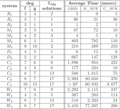
In order to evaluate the implementation we have performed tests with the polynomial sys-tems that are presented in section A.1. The performance of the implemented algorithms for bivariate solving is averaged over 10 iterations in maple 9.5 console and is shown in table 1. Polynomial systems Ri, Mi,and Diare presented in [ET05], systems Ci in [GVN02], and
Wi are the Ci after swapping the x and y variables. Note that systems Ci and Wi are of
the form f = ∂f∂y = 0 that arise in the topology of real plane algebraic curves. Finally, the polynomial system W5is not generated since the initial curve is a symmetric polynomial.
system fdegg Ralg Average Time (msecs) solutions grid m_rur g_rur
R1 3 4 2 5 9 5 R2 3 1 1 66 21 36 R3 3 1 1 1 2 1 M1 3 3 4 87 72 10 M2 4 2 3 4 5 4 M3 6 3 5 803 782 110 M4 9 10 2 218 389 210 D1 4 5 1 6 12 6 D2 2 2 4 667 147 128 C1 7 6 6 1, 896 954 222 C2 4 3 6 177 234 18 C3 8 7 13 580 1, 815 75 C4 8 7 17 5, 903 80, 650 370 C5 16 15 17 >20′ 60, 832 3, 877 W1 7 6 9 2, 293 2, 115 247 W2 4 3 5 367 283 114 W3 8 7 13 518 2, 333 24 W4 8 7 17 5, 410 77, 207 280
Table 1: Performance averages over 10 runs in maple 9.5 on a 2GHz AMD64@3K+ processor with 1GB RAM.
Recall that computations are performed first using intervals with floating point arithmetic (as it was described in section 6.1) and, if they fail, then an exact algorithm using rational arithmetic is called. For GCD computations in an extension field the maple package of [vHM02] is used. Finally, also note that the optimal algorithms for computing and evaluating polynomial remainder sequences have not yet been implemented. Hence, it is reasonable to expect more efficient computations on a future release of the library.
It seems that g_rur is the solver of choice since it is faster than grid and m_rur in 17 out of the 18 instances. However, this may not hold when the extension field is of high
degree. g_rur yields solutions in less than a second, apart from system C5. Overall, for
total degrees≤ 8, g_rur requires less than 0.4 secs to respond. On average, g_rur is 7-11 times faster than grid, and about 38 times than m_rur. The inefficiency of m_rur can be justified by the fact that m_rur solves sheared systems which are dense and of increased bitsize w.r.t. the original systems. Finally, it should be noted that grid reaches a stack limit with the default maple stack size (8, 192) when trying to solve system C5. However,
even when we increased the stack ten times, grid could not yield all solutions within 20 minutes. Setting the stack size to the required limit can be done with the following maple command:
kernelopts(stacklimit=81920);
6.2.1 Comparing slv solvers
The following two paragraphs will briefly compare g_rur with grid and m_rur in bivari-ate solving.
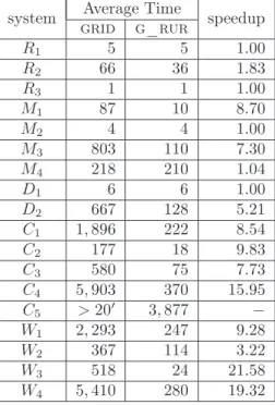
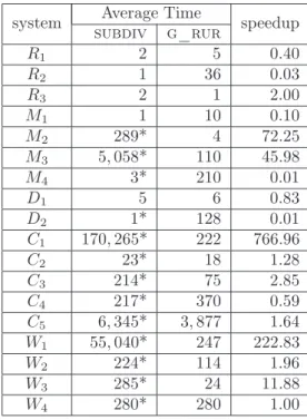
g_rur vs. grid Table 2 presents running times for bivariate solving between grid and g_rur. The final column in this table indicates the speedup that is achieved when preferring g_rur for bivariate solving. In other words, speedup = TIMEgrid
TIMEg_rur.As it is shown from the table g_rur can be up to 21.58 times faster than grid with an average speedup of around 7.27 among the input systems and excluding system C5 where grid
failed to reply within 20 minutes. Moreover, in terms of total computing times for the entire test-set (again excluding system C5) we can observe that:
• Total time for grid = 19, 001 msecs. • Total time for g_rur = 1, 860 msecs.
In other words, the speedup in terms of total computing time is about 10.22.
g_rur vs. m_rur Table 3 presents running times for bivariate solving between m_rur and g_rur. Similarly with the previous table, the final column indicates the speedup that is achieved when preferring g_rur for bivariate solving. As it is shown from the table g_rur can be up to 275.74 times faster than m_rur with an average speedup of around 38.01 among the input polynomial systems. Moreover, in terms of total computing times for the entire test-set we can observe that:
• Total time for m_rur = 227, 862 msecs. • Total time for g_rur = 5, 737 msecs.
system Average Time speedup grid g_rur R1 5 5 1.00 R2 66 36 1.83 R3 1 1 1.00 M1 87 10 8.70 M2 4 4 1.00 M3 803 110 7.30 M4 218 210 1.04 D1 6 6 1.00 D2 667 128 5.21 C1 1, 896 222 8.54 C2 177 18 9.83 C3 580 75 7.73 C4 5, 903 370 15.95 C5 >20′ 3, 877 − W1 2, 293 247 9.28 W2 367 114 3.22 W3 518 24 21.58 W4 5, 410 280 19.32
Table 2: The performance of grid and g_rur implementations on bivariate solving and the speedup that is achieved when choosing g_rur.
In other words, the speedup in terms of total computing time is about 39.72.
Again, it should be noted that m_rur solves sheared systems which are dense and of increased bitsize. In addition to that, since the polynomial systems are sheared (whenever necessary) in m_rur’s case, m_rur also computes the multiplicities on the intersections. A more accurate comparison will follow when all solvers will compute solutions on the same sheared systems and hence all of them will be able to decide the multiplicities on the intersections.
6.2.2 Decomposing running times
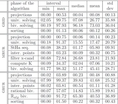
The following paragraphs demonstrate the decomposition of computing-time required by each algorithm in its respective major function calls as these timings were measured in the test-bed polynomial systems. Table 5 presents detailed statistics of every algorithm on every polynomial system from the test-set, while table 4 tries to capture the basic statistical properties of the previous table.
The major function calls and thereby the decomposition of running times and the respec-tive entries on the above tables can be summarized as follows. Projections shows the time
system Average Time speedup m_rur g_rur R1 9 5 1.80 R2 21 36 0.58 R3 2 1 2.00 M1 72 10 7.20 M2 5 4 1.25 M3 782 110 7.11 M4 389 210 1.85 D1 12 6 2.00 D2 147 128 1.15 C1 954 222 4.30 C2 234 18 13.00 C3 1, 815 75 24.20 C4 80, 650 370 217.97 C5 60, 832 3, 877 15.69 W1 2, 115 247 8.56 W2 283 114 2.48 W3 2, 333 24 97.21 W4 77, 207 280 275.74
Table 3: The performance of m_rur and g_rur implementations on bivariate solving and the speedup that is achieved when choosing g_rur.
for the computation of the resultants, Univ. Solving for real solving the resultants, and Sortingfor sorting solutions. In grid’s and m_rur’s case, biv. solving corresponds to matching. In g_rur’s case timings for matching are divided between rational biv. and Ralg biv.; the first refers to when at least one of the co-ordinates is a rational number,
while the latter indicates timings when both co-ordinates are not rational. Inter. points refers to computation of the intermediate points between resultant roots along the y-axis. StHa seq.refers to the computation of the StHa sequence. Filter x-cand shows the time for additional filtering. Compute K reflects the time for sub-algorithm compute-k.
In a nutshell, grid spends more than 73% of its time in matching. Recall that this percent includes the application of filters and does not take into account the polynomial system C5 where grid failed to reply within 20 minutes. m_rur spends about 45-50% of
its time in matching and about 24-27% in the pre-computation filtering technique. g_rur spends 55-80% of its time in matching, including gcd computations in an extension field.
Note also the significance of table 5 in order to draw further conclusions regarding the current implementation. Table 4 provides a mean of around 6% for the computation of the StHa sequence of f and g required by m_rur. However, we can observe that this step
phase of the interval median
mean std algorithm min max dev
g r id projections 00.00 00.53 00.04 00.08 00.13 univ. solving 02.05 99.75 07.08 26.77 35.88 biv. solving 00.19 97.93 96.18 73.03 36.04 sorting 00.00 01.13 00.06 00.12 00.26 m r u r projection 00.00 00.75 00.06 00.14 00.23 univ. solving 00.18 91.37 15.55 17.47 20.79 StHa seq. 00.08 38.23 01.17 05.80 09.91 inter. points 00.00 03.23 00.09 00.32 00.75 filter x-cand 00.68 72.84 26.68 23.81 21.93 compute K 00.09 34.37 02.04 07.06 10.21 biv. solving 01.77 98.32 51.17 45.41 28.71 g r u r projections 00.02 03.89 00.23 00.48 00.88 univ. solving 07.99 99.37 39.83 41.68 25.52 inter. points 00.02 03.81 00.54 01.11 01.28 rational biv. 00.07 57.07 14.83 15.89 19.81 Ralg biv. 00.00 91.72 65.30 40.53 36.89 sorting 00.00 01.50 00.22 00.32 00.43
Table 4: Statistics on the performance of slv’s algorithms in bivariate solving.
might very well take up to 38.23% of the total computing time. Indeed, a closer look on table 5 reveals that this is the case for the difficult system C5.Moreover, by table 1 we can
observe that m_rur requires about 61 seconds to solve system C5. Hence, we can obtain
a practical lower bound of about 23 seconds for m_rur in this case, which is already bad compared to the performance of g_rur for the entire problem (solving the system). This is a consequence and also a reminder for future work on the implementation of optimal algorithms on subresultant and Sturm-Habicht sequences. As a very important sidenote it should be stressed that implementing these optimal algorithms in sequences computations, the overall performance results for all solvers will be improved since the entire library is based on Sturm sequences to perform computations, such as pure univariate solving (root isolation), comparison of real algebraic numbers, and univariate and bivariate sign determination of functions evaluated respectively over one or a pair of real algebraic numbers.
a te re a l so lv in g S y st e m P ro je ct io n s U n iv a ri a te B iv a ri a te P ro je ct io n o n x -a x is U n iv a ri a te S tH a S e q u e n ce In te rm . P o in ts F il te ri n g o n x -a x is C o m p u te K F IN D (B iv . S o l. ) P ro je ct io n s U n iv a ri a te In te rm . P o in ts R a ti o n a l B iv a ri a te Ra lg B iv a ri a te R1 0.19 73.71 25.78 0.06 28.30 17.91 0.64 1.21 19.79 32.09 0.22 53.75 2.08 43.71 0.02 R2 0.01 4.47 95.52 0.00 16.30 0.61 0.09 72.84 3.50 6.66 0.07 7.99 0.12 0.10 91.72 R3 0.53 78.46 20.84 0.17 33.04 20.01 0.97 2.79 27.45 15.57 0.67 40.29 1.85 57.07 0.04 M1 0.04 10.13 89.75 0.05 21.06 1.46 0.14 35.63 2.97 38.69 0.14 79.62 2.83 16.13 0.02 M2 0.13 56.29 42.45 0.12 32.57 9.49 3.23 0.68 34.37 19.54 0.48 39.83 3.81 55.07 0.00 M3 0.00 4.98 95.02 0.02 7.39 0.16 0.02 60.60 1.18 30.62 0.03 28.60 0.67 0.50 70.14 M4 0.06 99.75 0.19 0.74 91.37 0.44 0.00 1.25 4.43 1.77 0.07 99.37 0.03 0.54 0.00 D1 0.11 95.25 4.61 0.06 33.81 9.47 0.20 21.14 19.57 15.75 1.20 81.26 0.54 16.93 0.00 D2 0.01 3.80 96.18 0.00 15.55 0.31 0.11 57.51 1.99 24.53 0.02 17.94 0.22 0.07 81.69 C1 0.04 2.69 97.27 0.27 5.02 2.37 0.04 28.19 2.02 62.09 0.23 21.00 0.16 2.32 76.25 C2 0.02 6.60 93.32 0.01 9.40 0.44 0.08 20.57 2.04 67.46 0.22 75.83 2.47 21.08 0.01 C3 0.01 2.88 97.03 0.04 2.05 1.17 0.00 28.66 1.62 66.46 0.33 16.47 0.16 14.83 67.69 C4 0.18 2.07 97.74 0.02 0.18 0.08 0.00 1.30 0.09 98.32 0.55 33.57 0.32 3.23 62.00 C5 − − − 0.75 1.92 38.23 0.00 6.43 1.49 51.17 3.89 30.43 0.02 0.35 65.30 W1 0.04 2.67 97.27 0.07 3.60 1.03 0.02 26.68 1.47 67.13 0.04 20.56 0.16 1.66 77.55 W2 0.00 7.08 92.89 0.00 11.02 0.22 0.18 39.44 1.72 47.42 0.03 21.78 0.27 0.95 76.89 W3 0.02 2.18 97.73 0.05 1.63 0.94 0.00 22.26 1.27 73.84 0.41 48.02 3.69 46.37 0.00 W4 0.01 2.05 97.93 0.00 0.23 0.12 0.00 1.36 0.10 98.19 0.02 33.85 0.51 5.17 60.18 ° 6 1 1 6
6.2.3 The effect of filtering
In the following paragraphs we measure the effect of interval arithmetic filters.
grid Table 6 presents running times for grid solver in cases where no filtering is performed in computations, i.e. all computations rely on Sturm sequences, or all filters have been applied as these were described in section 6.1. The final column speedup indicates the speedup achieved by filters in every case. Based on the numbers of the above table, the
sy
st
e
m deg
so
ls Average Time (msecs)
Speedup SLV-grid f g NO FILTERS FILTERED R1 3 4 2 5 5 1.00 R2 3 1 1 41 66 0.62 R3 3 1 1 1 1 1.00 M1 3 3 4 22 87 0.25 M2 4 2 3 4 4 1.00 M3 6 3 5 1, 231 803 1.53 M4 9 10 2 262 218 1.20 D1 4 5 1 6 6 1.00 D2 2 2 4 583 667 0.87 C1 7 6 6 2, 601 1, 896 1.37 C2 4 3 6 65 177 0.37 C3 8 7 13 106 580 0.18 C4 8 7 17 35, 168 5, 903 5.98 C5 16 15 17 >20′ >20′ − W1 7 6 9 2, 895 2, 293 1.26 W2 4 3 5 514 367 1.40 W3 8 7 13 104 518 0.20 W4 8 7 17 35, 054 5, 410 6.48
Table 6: Performance averages over 10 runs in maple 9.5 on a 2GHz AMD64@3K+ processor with 1GB RAM.
average speedup achieved by filtering techniques is about 1.51. However, in terms of total computing time for the entire test-set we can observe that:
• Total time without filtering = 78, 662 msecs. • Total time with filtering = 19, 001 msecs.
Hence, the speedup achieved for the entire test-set is about 4.14. Note that in both of the above computations system C5has been excluded since neither variation of grid was able to
solve the system within 20 minutes. However, there are indications that filtering techniques help more in other cases, see for example section 6.4.3.
m_rur The effect of filtering techniques in the case of m_rur will be discussed in section 6.4.3 where all solvers deal with bivariate systems in generic position.
g_rur A similar table with that in the case of grid is table 7. This time the average
sy
st
e
m deg
so
ls Average Time (msecs)
Speedup SLV-g_rur f g NO FILTERS FILTERED R1 3 4 2 6 5 1.20 R2 3 1 1 36 36 1.00 R3 3 1 1 1 1 1.00 M1 3 3 4 10 10 1.00 M2 4 2 3 4 4 1.00 M3 6 3 5 141 110 1.28 M4 9 10 2 201 210 0.96 D1 4 5 1 6 6 1.00 D2 2 2 4 171 128 1.34 C1 7 6 6 236 222 1.06 C2 4 3 6 18 18 1.00 C3 8 7 13 75 75 1.00 C4 8 7 21* 382 370 1.03 C5 16 15 17 3, 861 3, 877 1.00 W1 7 6 9 277 247 1.12 W2 4 3 5 141 114 1.23 W3 8 7 13 24 24 1.00 W4 8 7 17 318 280 1.13
Table 7: Performance averages over 10 runs in maple 9.5 on a 2GHz AMD64@3K+ processor with 1GB RAM.
speedup achieved by filtering is about 1.08. In terms of total computing time for the entire test-set we can observe that:
• Total time without filtering = 5, 908 msecs. • Total time with filtering = 5, 737 msecs.
In other words, the speedup that is achieved by filtering for the entire test-set is about 1.03. Thus g_rur seems not to be affected at a significant level by filtering. However,
this is more or less expected since g_rur relies heavily on gcd computations in extension fields and maple’s built-in function for factoring. Even when computing the multiplicities of the given system, g_rur seems not to be affected much from filtering. For a more concrete comparison, please refer to section 6.4.3 that discusses the problem of computing the multiplicities of the given system.
6.3
Bivariate solving and other packages
For the sake of completeness on the evaluation of the initial release of the slv library tests have been made with other solvers on the same polynomial systems. First of all, fgb/rs
2
[Rou99], which performs exact real solving using Gröbner bases and RUR, through its maple interface has been tested. It should be underlined though that communication with maple increases the runtimes and additional tuning might offer 20-30% efficiency increase. Moreover, 3 synaps3
solvers have been tested: sturm is a naive implementation of grid [ET05]; subdiv implements [MP05], and is based on Bernstein basis and double arithmetic. It needs an initial box for computing the real solutions of the system and in all the cases the box [−10, 10] × [−10, 10] was used. newmac [MT00], is a general purpose solver based on computations of generalized eigenvectors using lapack, which computes all complex solutions.
Other maple implementations have also been tested: insulate is a package that im-plements [WS05] for computing the topology of real algebraic curves, and top imim-plements [GVN02]. Both packages were kindly provided by their authors. We tried to modify the packages so as to stop them as soon as they compute the real solutions of the corresponding bivariate system and hence achieve an accurate timing in every case. Finally, it should be noted that top has an additional parameter that sets the initial precision (decimal digits). A very low initial precision or a very high one results in inaccuracy or performance loss; but there is no easy way for choosing a good value. Hence, we followed [Ker06] and recorded its performance on initial values of 60 and 500 digits.
It should be underlined that experiments are not considered as competition, but as a crucial step for improving existing software. Moreover, it is very difficult to compare different packages, since in most cases they are made for different needs. In addition, accurate timing in maple is hard, since it is a general purpose package and a lot of overhead is added to its function calls. For example this is the case for fgb/rs.
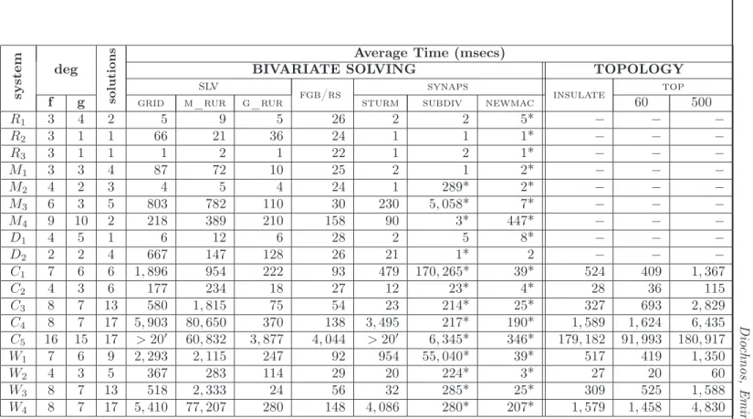
Overall performance results are shown on tab. 8, averaged over 10 iterations. Although the current solver of choice for slv library is g_rur, the other solvers are presented as well for completeness. Note that for the first data set, there are no timings for insulate and top since it was not easy to modify their code so as to deal with general polynomial systems. The rest (systems Ci and Wi) correspond to algebraic curves, i.e. polynomial systems of the
form f = ∂f∂y = 0, that all packages can deal with.
2
http://www-spaces.lip6.fr/index.html
3
In cases where the solvers failed to find the correct number of real solutions we indicate so with an asterisk (*). In the case of newmac where all complex solutions are computed, the (*) is placed in one more case: since newmac computes all complex solutions, a further computing step is required so as to distinguish the ones that reflect the real solutions.
D io ch n o s, E m iri s a n d T sy st e m deg s o lu t io n s
Average Time (msecs)
BIVARIATE SOLVING TOPOLOGY
slv
fgb/rs synaps insulate top
f g grid m_rur g_rur sturm subdiv newmac 60 500
R1 3 4 2 5 9 5 26 2 2 5* − − − R2 3 1 1 66 21 36 24 1 1 1* − − − R3 3 1 1 1 2 1 22 1 2 1* − − − M1 3 3 4 87 72 10 25 2 1 2* − − − M2 4 2 3 4 5 4 24 1 289* 2* − − − M3 6 3 5 803 782 110 30 230 5, 058* 7* − − − M4 9 10 2 218 389 210 158 90 3* 447* − − − D1 4 5 1 6 12 6 28 2 5 8* − − − D2 2 2 4 667 147 128 26 21 1* 2 − − − C1 7 6 6 1, 896 954 222 93 479 170, 265* 39* 524 409 1, 367 C2 4 3 6 177 234 18 27 12 23* 4* 28 36 115 C3 8 7 13 580 1, 815 75 54 23 214* 25* 327 693 2, 829 C4 8 7 17 5, 903 80, 650 370 138 3, 495 217* 190* 1, 589 1, 624 6, 435 C5 16 15 17 >20′ 60, 832 3, 877 4, 044 >20′ 6, 345* 346* 179, 182 91, 993 180, 917 W1 7 6 9 2, 293 2, 115 247 92 954 55, 040* 39* 517 419 1, 350 W2 4 3 5 367 283 114 29 20 224* 3* 27 20 60 W3 8 7 13 518 2, 333 24 56 32 285* 25* 309 525 1, 588 W4 8 7 17 5, 410 77, 207 280 148 4, 086 280* 207* 1, 579 1, 458 4, 830
6.3.1 g_rur and other solvers
In the following paragraphs we will try to compare the performance of g_rur with the rest of the solvers. For this purpose, we conduct speedup-tables like the ones that were drawn in section 6.2.1.
g_rur vs. fgb/rs Table 9 presents running times for fgb/rs and g_rur as well as the speedup that one gains when choosing g_rur instead of fgb/rs for bivariate solving. As it is shown from the table g_rur is faster than fgb/rs in 8 out of the 18 instances,
system Average Time speedup fgb/rs g_rur R1 26 5 5.20 R2 24 36 0.67 R3 22 1 22.00 M1 25 10 2.50 M2 24 4 6.00 M3 30 110 0.27 M4 158 210 0.75 D1 28 6 4.67 D2 26 128 0.20 C1 93 222 0.42 C2 27 18 1.50 C3 54 75 0.72 C4 138 370 0.37 C5 4, 044 3, 877 1.04 W1 92 247 0.37 W2 29 114 0.25 W3 56 24 2.33 W4 148 280 0.53
Table 9: The performance of fgb/rs and g_rur on bivariate solving and the speedup that is achieved when choosing g_rur.
including the difficult system C5. The speedup factor ranges from 0.2 to 22 with an average
of 2.62. However, in terms of total computing times for the entire test-set we can observe that:
• Total time for fgb/rs = 5, 044 msecs. • Total time for g_rur = 5, 737 msecs.