Structural Path Analysis and Multiplier Decomposition within a Social Accounting Matrix Framework

Structural Path Analysis and Multiplier Decomposition within a Social Accounting Matrix Framework

Author(s): Jacques Defourny and Erik Thorbecke

Source: The Economic Journal, Vol. 94, No. 373 (Mar., 1984), pp. 111-136 Published by: Blackwell Publishing for the Royal Economic Society

Stable URL: http://www.jstor.org/stable/2232220 . Accessed: 13/04/2011 11:23

Your use of the JSTOR archive indicates your acceptance of JSTOR's Terms and Conditions of Use, available at .

http://www.jstor.org/page/info/about/policies/terms.jsp. JSTOR's Terms and Conditions of Use provides, in part, that unless you have obtained prior permission, you may not download an entire issue of a journal or multiple copies of articles, and you may use content in the JSTOR archive only for your personal, non-commercial use.

Please contact the publisher regarding any further use of this work. Publisher contact information may be obtained at .

http://www.jstor.org/action/showPublisher?publisherCode=black. .

Each copy of any part of a JSTOR transmission must contain the same copyright notice that appears on the screen or printed page of such transmission.

JSTOR is a not-for-profit service that helps scholars, researchers, and students discover, use, and build upon a wide range of content in a trusted digital archive. We use information technology and tools to increase productivity and facilitate new forms of scholarship. For more information about JSTOR, please contact support@jstor.org.

Blackwell Publishing and Royal Economic Society are collaborating with JSTOR to digitize, preserve and

extend access to The Economic Journal.

The Economic Journal, 94 (March 1984), 111-136

Printed in Great, Britain

STRUCTURAL

PATH ANALYSIS

AND

MULTIPLIER

DECOMPOSITION

WITHIN

A

SOCIAL

ACCOUNTING

MATRIX

FRAMEWORK

Jacques Defourny and Erik Thorbecke

The main purpose of this paper is to apply structural path analysis to a Social Accounting Matrix (SAM) framework. Because the SAM is a comprehensive -

essentially general equilibrium- data system, the whole network through which influence is transmitted can be identified and specified through structural path analysis. The latter provides an alternative and much more detailed way to decompose multipliers as compared with the traditional treatment of Stone

(I978) and Pyatt and Round (I979).

This paper consists of five sections. The first one reviews the SAM framework as a basis for multiplier analysis and multiplier decomposition. In particular, the additive decomposition in terms of transfer, open-loop and closed-loop effects is succinctly presented. Section II applies this conventional decomposition to a SAM of South-Korea to illustrate with eleven specific cases the effects of an exogenous injection on the endogenous accounts of the SAM, i.e. the incomes, of the factors, household groups and production activities.

Section III is devoted to the presentation of the elements of structural analysis and, more particularly, the transmission of economic influence within a structure. Finally, Section IV applies structural path analysis to the South-Korean SAM and compares and contrasts the multiplier decomposition which it yields, with the alternative decomposition discussed in Section II. The comparison is the more significant in that the two decomposition methods are applied to the same eleven selected cases spanning a variety of sectors (i.e. poles) of origin (for the injection) and sectors (poles) of destination.

The empirical analysis in Section TV suggests that structural path analysis applied to a SAM is a potentially operationally useful technique within which a whole series of policy issues can be addressed. The final section is devoted to a brief summary and conclusions.

I. THE SOCIAL ACCOUNTING MATRIX, MULTIPLIER

ANALYSIS AND DECOMPOSITION

The Social Accounting Matrix (SAM) has become used increasingly in the last years as a general equilibrium data system linking, among other accounts, pro- duction activities, factors of production and institutions (companies and house- holds). As such, it captures the circular interdependence characteristic of any economic system among (a) production, (b) the factorial income distribution (i.e. the distribution of value added generated by each production activity to the

II2 THE ECONOMIC JOURNAL [MARCH

Table I

Simplifed Schematic Social Accounting Matrix

Expenditures

Endogenous accounts Exog.

0

Production E S u

Factors Households activities : o H

I

~

L Sum of otlher accounts 4 t1 1 11 Yx

Totals 5 Yi Y' Y3 Yx

various factors), and (c) the income distribution among institutions and, parti- cularly, among different socio-economic household groups.'

Under certain assumptions, such as excess capacity (i.e. availability of unused resources) and fixed prices, the SAM can be used as the basis for simple modelling. More specifically, the effects of exogenous injections on the whole economic system can be explored by multiplier analysis which requires partitioning the SAM into endogenous and exogenous accounts. Typically the former include (i) factors; (ii) institutions (companies and households); and, (iii) production activities; while the exogenous accounts consist of (iv) government; (v) capital; and (vi) rest of the world.

Table I shows this partition and the transformations (matrices) involving the

three endogenous accounts. These matrices are, respectively, T13 which allocates the value added generated by the various production activities into income accruing to the factors of production; T33 which gives the intermediate input requirements (i.e. the input-output transactions matrix). T21 maps the factorial income distribution into the household income distribution (where households are distinguished according to socio-economic characteristics); T22 captures the income transfers within and among household groups; and finally T32 reflects the expenditure pattern of the various institutions (mainly the household groups) for

1 _{For a discussion of the structure of the SAM and its potential use in policy analysis as a data system}

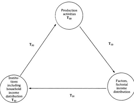
I984] STRUCTURAL PATH ANALYSIS ₁₁₃ Productio activities T32~ ~~~~3 Institu- tions Factors, including factorial household income income distribution distribution T21 T22

Fig. i. Simplified interrelationship among principal SAM accounts (production activities,

factors and institutions). Tij stands for the corresponding matrix in the simplified SAM

which appears on Table i. Thus, for exaniple, T13 refers to the matrix which appears at

the intersection of row i (account i), i.e. 'factors' and column 3 (account 3), i.e. 'production

activities. '

the different commodities (production activities) which they consume. Fig. I

shows this same triangular interdependence graphically using the same notation as in Table i.

In Table 2 the row totals for incomes received by endogenous accounts are given by (the column vector) yn, which consists of two parts arising from, respectively, (i) expenditures by the endogenous accounts recorded as Tnn and summed up as column vector n; and (ii) expenditures by the exogenous accounts recorded as Tnx and summed up as x.1 The latter part is referred to as injections. We have

Yn= n+x. (I)

Analogously for the incomes received by the exogenous accounts yx2 (see Table 2)

Yx = I+t. (2)

The elements of the endogenous transaction matrix Tnn in Table 2 can be

1 _{This section follows closely the notation given in Svejnar and Thorbecke (I983). See also for a}

similar treatment Pyatt and Round (1979), which uses, however, a somewhat different notation.

2 It is to be noted that because Table 2 is a SAM, its corresponding row and column totals are

equal - column totals for endogenous accounts are given by (the row vector) yn, while those for exogenous accounts are given by y'.

I 14 THE ECONOMIC JOURNAL [MARCH

Table 2

Schematic Representation of Endogenous and Exogenous Accounts in a SAM

Expenditures

Endogenous Exogenous E Totals

Injections

. | Endogenous Tn ? _{| n |} Yn

Leakages Residual balances

Exogenous _{Tx xxt} Y

Totals Y. Y

expressed as ratios oftheir corresponding column sums, i.e. as average expenditure

propensities,'

nn Any (3)

where Y is a diagonal matrix whose elements are yi, z _ I, ..., n. Similarly

Txn

By introducing the matrices An and Al, n and 1 can now be expressed as

n

= AnYn

(5)

and

1 = Aly.Y (6)

Combining (i) and (5) gives the multiplier matrix Man

Yn= Any+x= (I-A.)-lx = M,x. (7)

Equation (7) yields endogenous incomes (Yn) by multiplying injections (x) by a multiplier matrix Ma.2 This matrix has been referred to as the accounting multiplier matrix because it explains the results observed in a SAM and not the process by which they are generated.3

As described previously, and as a comparison of Tables I and 2 shows, T.. is

partitioned. Corresponding to this partition the matrix of average expenditure propensities is as follows,

oo A,3]

An= A21

01.

(8)

o A32 A33

At first glance the system specified in equations (7) and (8) appears analogous to the open Leontief model. In fact, the basic difference is that the SAM is closed

1 _{Hence, columns of A. in equation (3) show expenditures as proportions of total income (i.e. y' in}

Table 2) and not as absolute amounts as in Tnn.

1 _{More precisely, this equation yields the income levels of factors (y1), households (Y2) and production}

activities (ye) which are endogenously determined as functions of the exogenous injections (x).

3 See Pyatt and Round (I979) for the distinction between accounting multiplier matrix and fixed-

I984] STRUCTURAL PATH ANALYSIS ₁₁₅ with respect to the determination of the factorial and household income distri- bution and the consumption behaviour of households. In a SAM system, combining equations (7) and (8) and solving for the production activities vector

(yO) yields

Y3- A33y3 +(A32Y2 + X3) = (I-A33)-' (A32y2 + X3)* (9)

This formulation generalises the Leontief model by including as one of the elements of final demand the effects of income distribution (Y2) on household consumption (through A32 which reflects the consumption pattern of each group of households).'

One limitation of Ma as derived in equations (7) and (8) is that it implies unitary income elasticities (the prevailing average expenditure propensities in A. are assumed to apply to any incremental injection). A more realistic alter- native is to specify a matrix of marginal expenditure propensities (C. below) corresponding to the observed income and expenditure elasticities of the different agents, under the assumption that prices remain fixed when income is altered. Expressing equation (i) in terms of changes in injections, one obtains

dyn= dn+dx (Io)

=Cndyn+dx= (I-Cn) -dx =M,dx. (II)

MC has been coined the fixed-price multiplier matrix and its advantage is that it allows any non-negative income and expenditure elasticities to be reflected in Mc.2

A rearrangement of the well-known multiplicative decomposition converts the matrix of accounting multipliers (Ma) into four additive components, (i) the initial injection (I); (ii) the net contribution of the transfer multiplier effects (T); (iii) the net contribution of open-loop or cross multiplier effects (0) and (iv) the net contribution of circular closed-loop effects (C) ;3

Ma-I + (Mal-I) + (Ma2-I) Mal + (Ma3-I) Ma2Mal.

I + T + 0 + C (I2)

The transfer effects capture the multiplier effects resulting from direct transfers within endogenous accounts (in our particular case among institutions and households (A22) and the interindustry transfers (A33)). The open-loop effects capture the interactions among and between the three endogenous accounts, while the closed-loop effects ensure that the circular flow of income is completed among endogenous accounts, i.e. from production activities to factors to insti- tutions and then back to activities in the form of consumption demand following the triangular pattern presented in Fig. I.

1 _{In contrast, the open Leontief model can be expressed as follows using the same notation}

Y3 = (I-A33)-1 f, where A33 is the input-output coefficient matrix and f is exogenous final demand. It is obvious that (g) contains more information and a higher degree of endogeneity since it captures the effects of income distribution on consumption which the Leontief formulation does not.

2 _{Given the average expenditure propensities from the initial (base year) SAM table and a know-}

ledge of the respective income elasticities, marginal expenditure propensities can be directly derived.

3 For a detailed discussion and derivation of multiplier decomposition, see Pyatt et al. (1977);

ii6 THE ECONOMIC JOURNAL [MARCH

It will be shown shortly that the above multiplier decomposition reveals only to a very limited extent how influence is transmitted within a structure. Because of the partitioning into three endogenous accounts, it can only decompose the effects of injections into total effects within and between accounts. As such it cannot identify the network of paths along which influence is carried among and between production activities, factors and households - which is the contribution of structural path analysis as shown in Sections III and IV.

II. MULTIPLIER DECOMPOSITION APPLIED TO SOUTH-KOREAN SAM

Before turning to structural path analysis the above multiplier analysis and decomposition is applied by way of illustration to a SAM which was built for South-Korea (i968).' The A matrix of this SAM appears in a truncated form in Table 3.2 It can be seen that the factor account is broken down into I 5 categories, i.e. six different labour skills, two types of self-employed, capital, five types of farmers and government workers. The classification of households is essentially similar to that of factors.3 Production activities were divided into 29 activities on the basis of product-cum-technology characteristics. The other accounts (i.e. the exogenous ones) appearing in the SAM in Table 3 are government, capital and rest of the world.4 The South-Korean SAM is meant only to capture in an approximate way the structure of the economy of South-Korea in I 968. It is used here only for demonstrational and illustrative purposes.

In Table 4, eleven cases are selected to illustrate the effects of an injection in one sector on another via the respective accounting multipliers. Table 4, further- more, gives the decomposition of the multipliers into transfer effects, open loop effects and closed loop effects. These eleven cases are discussed very briefly in this section since they are analysed, in detail, on the basis of a different type of decomposition (i.e. structural path analysis) in Section IV. In fact, the purpose of this section is to illustrate the traditional multiplier decomposition as a back- ground against which the alternative structural path analysis decomposition can be presented in Section IV.

The first two cases (I and II) in Table 4 involve the effects of an injection in one production activity on another. The initial injection could consist of government expenditure or export demand. Thus, for example, it can be asked what the consequences would be of an injection of ioo units (won) of exogenous demand (say, export demand) for mining products on 'other agriculture' (non-cereal)

1 _{This SAM was built by Thorbecke based on the Adelman and Robinson (I978) data set as part of}

an NSF project dealing with the macroeconomic effects of the choice of technology. For detailed discussion of this SAM and, in particular, the attempt to distinguish activities according to product-

cum-technology characteristics, see part 4 of Svejnar-Thorbecke (I983).

2 _{To save space, Table 3 includes all the rows of the SAM but only selected columns, i.e. 3 factors,}

3 household groups, 4 production activities and the exogenous accounts. The complete A matrix can

be found in Svejnar and Thorbecke (I983). The corresponding accounting multipliers' Table is

available upon request from the authors.

3 _{It should be noted that the only institutions are households. Companies do not appear explicitly in}

the South-Korean SAM, instead the factors' account receives the capital value added and distributes to households directly.

4 _{It can readily be ascertained that the A matrix (average expenditure propensities) in Table 3 has}

Partial SAM Table for South Korea, 1968-Partial Matrices of Avo Endogenous I Factors of production l | ~~~~Engineers (l )| l l l Technicians (2) U Skilled workers (3) .? Apprentices (4) Unskilled workers (5) White-collar workers (6) Self-employed in manufacturing (7) I

~

o Agricultural labourers (I0)

vd Farm size I(I)

44~~~~~~~~~~~~~~~~~~~~~~~-

Farm size 2 2 II

Farm size 3 (1I3)

Farm size 4 (14)

Government workers (1I5)

Engineers (i 6) | | |

Z Technicians (2I 7) o 0-827 o o

CZ Skilled workers (I8) 0-0 0-0 0-0

Apprentices (I9) o-o 0-0 0-0

t'd Unskilled workers (20) 0-0 0-0 0-0 o

_ White-collar workers (2I) 010 0- I04 0-

o1. Self- n In manufacturing (22) o o oo o

employed In services (23) o o oo o

Capitalist (24) 0-079 o-oo8 o o

Agricultural labourers (25) 0o 0)0 0 0-0

.Z Farm size i (26) o o oI000

Farm size 2 (27) 0X0 0-0 0-0 Farm size 3 (28) o o oo o Farm size 4 (29) o4 o oo o Government workers (30) 0 392 0-059 o o Cereals (3I) 0 Other agriculture (32) Fishing (33) Processed foods (L) (34)

Processed foods (S + M + Self) (35)

Mining (36)

Textiles (9) 0037)

Textiles (Sw+oM+ self) (38) Finished textile products (39) Lumber andufurniture (42)

e Chemical products (L) (4

Chemical products (S + M+ self2 (42)

Energy (L +M) (43)

M _{Energy (S +self)} (44)

3 C A Cement, non-metallic mineral products (25)

FMetal products (L+(M) (46) Metal products (S+self) (47)

o.4 Machinery (48)

iTransport equ (49)

Pevrocessed foods (L) c (34)

Textilges (S+M+self) + slf (38 )

Finihed textiler products (39)

Chemircalipodutn L (53)

Metal produtse LM (546)

Table 3

ble for South Korea, 1968-Partial Ma trices of Average Expenditure Propensities for Endogenous Acco _{unts (An) an}

Endogenous Expenditures Propensites

I Factors of production 2 Households 3 Production activities

0.)~~~~~~~~

I~~~~r C I

00

(2) 00 0-0 5

(3)~~~ 0 o3 '0z 3

(4) ooo. o o onoo3 o oo7

(8) 'w 0o oo o

(9) 0@29} o 303 o I2I o8+ >

1 2 1i x8 19 20 32 33 34 35(

(x)

~~~~ ~~~~~~~~~~~~

(2) 0oo o 05 o'oo6 o'oo6

(3) 0'0 0'020 0c031 0'027

(4) 0o0 I 004 0'003 0'007

(3) oog o0o82 o'ox6 0'030

(6) o0o 0050 0o014 0o029

ring (7) 0_041 0_0 00 0o10o

(8) O'O 000 0'0 0'0

(7) 0o291 0o303 01 21 0o84

(io) ooo 0oo 0'038 00

20x) 0'099 0'0 o'0 o'o

(12) 00090 000 00 00

(13) o-0 o'096 0r0 0'0

(14) 0_043 0'0 0ro o_ o

(15) 0o0 0o0 ooo 00

(x6) 0?529 0?002 00

(17) 0o0 0'827 0o0

(i8) cro 00 0o0

(19) ?0? o'o . 0. (20) o'0 0ro c0, (21) 0'O 0-I04 0'0

(22) 0'O 10o o'o (23) 0o0 16o 20I

(24) 0'079 o1oo8 0o0

(25) 0o0 0ro 000

(26) ?ro oSo oo000

(27) 0o4 0'0 0Io (28) 000 0'0 0o0 (29) 000 000 00? (30) 0'392 0I059 00'

(31) o'o6i O'022 _o0197 O'102 030 o'oo8 o'oo8 70o8

(32) 0-124 O'144 0'I22 0'141 o'oz6 00236 0r236 466'

(33) 0'023 o'023 o'ox8 0 0 '0 01 o66 o'o66 7 1'08

t (342) 00o'os o o0osg5 0046 O'003 0005 _o'o65 oo65 3087'

if) ₍₃₅₎ 0-043 0'051 0'040 0'002 00004 0o0o6 0o056 266'3

(36) 0o0 0'0 oo o'oor oooo6 0o004 oroo6 x98'

(37) ~~~~~0'002 0'002 0rooi cro croox cro o'o 6-93

(38) 0'002 0'001 0'001 0-0 0'0 010 0'0 3'87 (39) o'o65 0'075 0078 0o003 0o034 0o004 o0004 170'

(40) 0oox o0002 0'00I 0'002 0007 I 002 0002 3416

(41) 0o014 0o017 0014 0o015 o'002 0?017 0?017 118(

- self) (42) 0'004 0-005 0'004 0-0o3 0.0 0-004 0'004 271'

(43) O'021 0023 0022 0'001 0o036 o'oi6 o ox6 273:

(44) 0'003 0I004 0o003 o4 o 0I003 o'oo6 0I003 427'1

ral products ₍₄₅₎ 0'002 O'002 0roo0 8 os 0'0 0'002 r0002 131', (46) o0o0I 0'02 0'001 7 rooB _{0 0003} 0-004 ₀₅₀₀₄ 121'

(47) o o00 o0001 0 o0 0ooi 0'001 0001 41'6

(48) 0'004 00O1 2 0.005 0'0 0'0 0-003 0'003 931',

(49) 0o003 0'010 0'00,3 oo o'oo6 oo 0o 0 _807'o

re Propensities for Endogenous Accounts (An) and Exogenous Accounts (A,))*

Propensites Exogenous expenditures

Ids 3 Production activities 4 5 6

-~~~~~~~~~~~~~~~~~~~~ C~~~~~~~~~~~~~~~~~- - 0' I o o3 0oo4 to o o o7 I -e '00 O@I _{0-029 -474} 0'0 2904I 0'0 090x 87+ 7395 -2 8' 8+ > Total ___ C ~~~~c2 &E~~~~?- ____ Q d4 income 20 32 33 34 35 6i 62 63 64 6 010 0-011I o-oo6 0-004 19639-7 00 0 I 5 o-oo6 o-oo6 237749 2 010 0-020 0-031 0,027 _86oo6-9 0109 004 0-003 0-007 126664 01 0-182 o-ox6 0-030 i04686-0 010 0-050 0-014 0-029 142743-0 010 0-041 010 01010 _7395-87 0-0 010 010 0.0 ₇₈₃₇ I.9 0-291 0-303 01l21 0-084 558745-0 0-038 010 010 0-0 29132-3 0-099 0.0 0-0 0-0 60709-2 0-091 010 0-0 010 6 x 179-1 o0o96 o o 0o0 0o 0 66680-4 0-043 0o0 0o 0o0 0 38986-9 010 00 010 010 81720-0 528-512 528-5I2 12320-0 1074-93 1074-93 24948 8 4386-12 4386 12 101306-o 42-5918 42-59I8 980o 89 4180-12 4180o12 96085-8 ._ _ _ _ _ _ _ _ _ _ __ _ _ _ 7070-00 7070-00 I63433-0 1363-91 1363-91 31426-7 ______ _______ _______ 8932-56 8932.56 206186-0

o-687500 o-687500 I22527'0

1408-96 1408-96 3i648 i 4284 56 4284-56 96241P2 521000 52 10-00 I ₁ 7026 0 6599-81 6599-81 I477460o 2956-84 2956-84 66195-0 4337q19 4337q19 100391-0

0-197 0-102 0'0 o-oo8 o-oo8 708- 166 -11724-9 1 12 000 -10904'7 285056-o

0-I 22 0-141 o-o16 0-236 0-236 466-054 771-884 3054-00 4291I94 29588o-o

o-oz8 00 0o 0 o-o66 o-o66 71-0000 44 8770 4425o00 4540 87 45409-I

0-046 0-003 0o005 o-o65 o-o65 308-284 425-145 6493-86 7227-29 91979 5

0-040 0002 0o004 o0o06 0o-o6 266-615 3674681 5616-13 6250-43 79544-1

0-0 O0OO1 0-004 o-oo6 o-oo6 198-000 1579-67 8583-00 10360o7 45027-0

0-001 0-0 o0001 0o0 0o0 6-93577 1 0826-I 11274-8 22107-8 85835-0

0'001 0-0 0'0 0-0 0o 0 3-87316 6045-65 6296-21 12345 7 47934-0

0-078 0003 0034 0-004 ?0004 170-036 I640'50 37136-o 38946s5 1 I4861'0

0001 0-002 0o007 0-002 0002 546-857 1874-58 19319-0 21740'4 53206-5

0'014 0'015 0002 0-017 0-017 i186-97 945 357 675-363 2807-69 55635-2

0-004 0-003 00 0-004 0-004 271 779 216-458 154-637 642-874 12738 4

0'022 0-001 0-036 o-oi6 o-oI6 2737 75 511I489 2650-95 5900-19 93449-0

0-003 0o0 o-oo6 0-003 0-003 427-608 79-8893 414'051 921-548 14595*2

01002 0-0 0'0 0-002 0'002 13 1390 5476-98 z86i-oo -3484-59 4546 i 5

0001 o-oo8 0-003 0o004 0-004 121* 50 5584663 2718 39 3398-21 57704 8

0'0 0-003 0-00I 01001 01001 41*6968 192-278 935-606 I1 69-58 1 9860-4

0o005 0o 0 00 0-003 0-003 931*883 15425-2 5287-00 2 I 644-1 6:398-4

0-003 0o0 o-oo6 0o0 0o 0 807-623 31374.7 405.000 32587-4 64241P2

00o46 o-0 oo -oor0 0-004 0-004 I 856-5 3 770$56 1883-66 7510 73 71x58746 o'o18 0? 0? 0002 oo 0-002 742-480 1507-97 753w338 3003-79 286309g 00o1 7 0-005 0-002 0-0 15 0o1 o _s x26 1 16 3 2 736 76 43 789-0 59 142 0 1 721I2 7-0

0'0 0'0 0'0 0@002 0'002 792900o 21t3775 8042-00 22974&0 2545970?

0-047 0o 0o 0o 0o oo 00 5508 89 0-0 5508-89 59983.9

Technicians (2) Skilled workers (3) Apprentices (4) Unskilled workers (5) S White-collar workers (6) cz Self-employed in manufacturing (7) I0 Self-employed in services (8) f :Capital (g)

o Agricultural labourers (io)

Cd _{Farm size} ! (I I) Farm size 2 (12) Farm size 3 (13) Farm size 4 (14) Government workers (15) Engineers (i6) 0529 0002 00

e Technicians (1 7) oo o0827 0o0

Skilled workers (x8) 00 00o 0o 0

s, Apprentices (19) cro 0oo o o

0 Unskilled workers (20) or o o 0o 0

r _3: White-collar workers (21) 0'O 0-104 ? o

-e

2 o Self- In manufacturing (22) o o 0o 0o 0

employed In services (23) or0 0o 0o0 0

0

v X Capitalist (24) 0079 o*oo8 0o0

e Agricultural labourers (25) 00 0o 0 0o 0

Z Farm size i (26) ro o oo000 *

v, Farm size 2 (27) or0 o0o o0o

< Farm size 3 (28) oo o o oo Farm size 4 (29) oo o o o 0o Government workers (30) 0392 0059 o 00 Cereals (31) Other agriculture (32) Fishing (33) Processed foods (L) (34)

Processed foods (S + M+ Self) (35)

Mining (36)

Textiles (L) (37)

Textiles (S+M+self) (38)

Finished textile products (39)

Lumber and furniture (40)

U Chemical products (L) (41)

Chemical products (S+ M+ self) (42)

.5 Energy (L+M)

o Energy (S + self) (44)

3 ₈ Cement, non-metallic mineral products (45)

Zs _{Metal products (S+ self) (47)}

0

o Machinery (48)

914

Transport equipment (49)

Beverages & tobacco (L) (5o)

Beverages & tobacco (S+M+self) (5a)

Other consumer products (52)

Construction (53)

Real estate (54)

Transportation & communication (55)

Trade and banking (S + M + L) (56)

Trade and banking (self) (57)

Education (58)

Medical, personal & other services (59)

Sub-total: 1 + 2 + 3 (6o) 100 1o000 1o000

4 Government income (6i) _ro oro o o

5 :Capital account (62) oro cro 00

6 Rest of the World (63) 0co cro _o

Sub-total: 4+ 5 + 6 (64) oo o0o0 roo

Total expenditures (65) 19640 23774 60709

* _{For reasons of space, only some of the columns are shown in the above truncated Table.}

contained in rows 6. 6I63, columns 1-59. Row gives total expenditures in millions of won fo

(2) 0-0 0o015 o'oo6 o-oo6

(3) 0o0 0'020 0-031 0'027

(4) 0-0 0'004 0o003 _o0007

(5) 0o0 o'I82 o'oI6 0o030

(6) 0o0 0o050 0o014 0o029

iring (7) 0o0 0'041 0-0 0-010

(8) 0o0 0'0 0o0 0o0

(9) 0'291 0I303 o'I21 o0o84

(I0) 0-038 0o0 o'o 0o0

(I I) 0-099 0'0 0-0 0-0

(12) o-09 I 0.0 0-0 0-0

(13) o-o96 0o0 o0o 0o0

(14) 0o043 0o0 o0o 0o0

(I5) 0o0 o'o o0o 0o0

(i 6) 0o529 0o002 0o0

( 7) 0o0 0-827 0o0

(I8) 0o0 o'o 0o0

(19) 0o0 0-0 0-0

(20) 0-0 0-0 0-0

(2 1) 0'0 0- I04 0o0

(22) 0o0 0o0 0o0

(23) 0o0 00 00

(24) 0-079 o-oo8 0o0

(25) 00 00 010

(26) 0o0 o'o 1I000

(27) 0o0 0o0 roo

(28) o0o o'o 0o0

(29) 0?0 ??o 0_0

(30) 0o392 0-059 0o0

(31) o-i6i 0'022 0'197 o'I02 0o0 o-oo8 o'oo8 708-

(32) 0o124 0-144 0'I22 0o141 o'oi6 o0236 0-236 466-'

(33) 0o023 0-023 o'oi8 o-o o0o o-o66 o-o66 7 I '0

(34) 0o050 0o059 0o046 0o003 0o005 o-o65 o-o65 308'

If') (35) 0o043 0o05 I 0'040 0'002 0004 o0os6 o0os6 266-

(36) 0o0 o'o 'o 0001 0o004 o-oo6 o-oo6 198-

(37) 0'002 0002 0-00I 0o0 0-001 o?; 0'0 6.93

(38) 0o001 0'00 I 0-001 0'0 0-0 0?0 0'0 3'87

(39) o-o65 0o075 0o078 0o003 0o034 _0?004 0?004 170-1

(40) 0o001 0002 0-00I 0o002 0-007 o'002 o0002 546.,

(41) o-014 0-017 0014 0015 0'002 0-017 O-017 I i8E

-self) (42) 0-004 0-005 o004 0-003 00 0?004 0?004 271'

(43) O'02I 0o023 O'022 0001 0o036 o-oi6 o-oi6 273;

(44) 0o003 0'004 0'003 0'o o*oo6 0'003 0o003 427-

ral products (45) O'002 0'002 0'002 0-0 0'0 0'002 0'002 ₁₃₁

(46) o00o1 0-002 0ol0I o-oo8 0o003 0o004 0o004 I21'

(47) o-o o-oo I 010 o-o3 ooo I 0-0 I 0-00 I I6

(48)

~

~~

0 00I 0 _0-003

0.001

00 00 ₄₁ 6

(48) 0-004 0o0 1 2 0-005 00 0'0 0003 0?003 93 I'

(49) Oo003 0o010 0-003 0o0 o-oo6 o?o ? o 807'

(5o) 0-041 0I050 o0046 o0oo I 0'001 0I004 0?004 I85(

I+self) (51) o-oi6 0'020 o'oi8 0-0 0'0 0'002 0'002 742.

(52) o-oi8 O'020 0-017 0-005 0-002 0-015 0'015 126]

(53) 0o0 o'o 0'o o oo 0o0 0'002 O'002 792C

(54) o0-054 o-o6 I o04 oo oo oo oo oo

ication)O'54 o'6i 0-047 0'0 0'0 0'0 010 0'0

cation ₍₅₅₎ o-o67 o-o84 0o055 o-oo6 0-007 0-0I4 0o014 473

+L) (56) 0-048 0o052 0o050 o0oog 0o017 0-025 0-025 147;

(57) o-o62 o-o67 o0o64 o0oI2 0'021 033 0033 I9I1

(58) 0-017 0o024 0o003 00 0o 0o0 0 0?0 3284

0erv7ces (59) o-o6i 0'075 0-053 o0ooI 0'002 0102 o'0 1 2 9464

(6o) _{i 0-ooo |000 1|000 0|905} 090o6 _{0|919 0|975 0o803 0'797 0'797 i6|85}

(6i) o0o 0o0 0o 0 0-041 o0039 0-042 0-001 _{0o004 0o037} 0o037 0o0

(62) 0o0 0o0 00 0o034 O'034 o0oI8 0o001 0-075 o-oog o9oog I 365

(63) 0-0 0o0 0o 0 0'020 O'021 0'021 0o022 0o117 0o157 0o157 3854

(64) 0-0 0o0 0o0 0-o5 0-094 o-o8i 0025 0'197 0'203 0-203 140(

(65) 1 9640 23774 60709 I0131 9802 96086 29588 45409 91980 79544 308

if the columns are shown in the above truncated Table. In the original Table (see Svejnar and Thorbecke (1983)) A, is contained i

9'Row 6 gives total expenditures in millions of won for each class and corresponds to column 6 which gives corresponding total expressed in millions of won.

0-0 0-015 ooo6 o-oo6 23774 2

0-0 0O020 0-031 0'027 86006-9

00 0o004 0o003 0o007 I 2666-4

0-0 oi82 o oI6 0-030 104686o

0-0 0*050 0-014 0o029 I 42743o

0.0 0-041 0-0 0-010 7395 87

0o0 0o0 0o0 0o0 7837 I 9

0-291 0?303 0-I21 o0o84 558745-0 0-038 0o0 o*o 010 29132-3 o-o99 o00 OO 0*0 60709-2 0-09 I 0.0 00 0-0 6i 179-1 o-o96 0.0 OO 0*0 6668o-4 0-043 0-0 00 00 38986-9 0*0 QO OO 010 8I720-o 528-512 528-512 12320-0 1074 93 1074 93 24948-8 4386- I 2 4386 I!2 10 I306-o 42-5918 42-59I8 980-I89 4180-12 4I80o12 96085-8 7070-00 7070-00 I63433-0 1363-91 1363-91 31426 7 8932 56 8932.56 206 i 86-o 0687500 o687500 122527-0 1408-96 14o8-96 3I648-i 4284-56 4284-56 96241-2 52I0-00 5210-00 1 I 7026-o 6599-81 6599-81 I477460o 2956-84 2956-84 66195- 4337'I9 4337'19 100391-0

0-197 o-I02 Qo o-oo8 o0oo8 708-I66 -I I724-9 I 12*000 -10904-7 285056-o

0 I22 0I141 oIoi6 o0236 0-236 466-054 771-884 3054-00 4291 94 295880-0

ooi8 0.0 Qo o-o66 o-o66 7I-0000 44 8770 4425-00 4540 87 45409gI

0046 0o003 0-005 o-o65 o-o65 308-284 425'145 6493 86 7227 29 91979 5

0O040 0-002 0004 o0o56 o0o56 266-6I5 367-68I 56 I 6I13 6250-43 79544 I

0-0 0o00o 0-004 o-oo6 o-oo6 198-000 1579 67 8583o00 10360-7 45027-0

0-001 0-0 0-001 0o;) 0o 6-93577 10826- I 11274-8 22107-8 85835-0

0-001 0-0 0-0 010 010 3-873I6 6045-65 6296-21 12345 7 47934 0

0078 0o003 0-034 0?o04 0004 170-036 I640-50 37136-o 38946 5 1 14861-0

O-OOI 0-002 0-007 0-002 0-002 546 857 1874 58 19319-0 217404 53206-5

0-014 0o015 0002 0-017 0-0I7 i I86-97 945 357 675 363 2807-69 55635-2

0004 0o003 00 0-004 0004 271779 216.458 154 637 642.874 I2738 4

0O022 0001 0o036 o-oi6 o-oi6 2737 75 511-489 2650-95 5900-19 93449 0

0-003 00 o-oo6 0.003 0 003 427-608 79-8893 414'051 921-548 14595'2

01002 0-0 00 0002 01002 131P390 -5476-98 i86ioo -3484 59 4546 I 5

0-ooI o-oo8 0o003 0?004 0?004 I 2I*I50 558.663 2718 39 3398-2 I 57704-8

0o0 0003 0001 O-OOI 0001 416968 192-278 935 606 1 I69-58 i9860o4

0005 0o 0 0.0 0 003 0?003 93 I .883 15425-2 5287-00 2 I 644-1 61398-4

0oOO3 0o0 o-oo6 o.o O.O 807-623 31374.7 405-000 32587 4 642412

0o046 o0oo I 0'001 0I004 0004 1856-51 3770-56 1883-66 75 I 0 73 7I587-6

o0oi8 0o0 0o0 o002 0O002 742-480 I507-97 753-338 3003'79 28630-9

0-0I7 0-005 o0002 0-015 0o0I5 126I6-3 2736 76 43789-o 5942-0 172127-0

01o 0o 0o 0 0-002 0-002 7929 00 213775 804200 229746-o 254597 0

0-047 0.0 010 0-0 00 00 5508-89 0.0 5508-89 59983-9

o0o55 o-oo6 0o007 O I4 0o0I4 4733 89 599 357 29822-0 35155-2 i65290-0

0o050 o-oog 0-017 0-025 0-025 14771I6 18554-2 4656-40 24687 8 147053O

oo64 OOI2 0O021 00-33 0033 19 I I84 24014-1 6026-60 31952 5 190323-0

0 003 0.0 010 0-0 00 32864-1 25 9289 010 32890oo 53768- I

0-O53 o0oo0 0'002 o-0I2 OO I 2 _{94696- I -I} 5269 I 8577-oo 88003-9 240803-0

Og9I9 O0975 o0803 O 797 0'797 I68231-0 3109020o 273339 0 752472-0 0-564488E+07

0-042 0 001 0-004 0-037 0-037 00 0-0 72300-0 72300-0 308301-0

o-o I8 0o001 0-075 o-oog ooog I 36220-0 010 I o8030o0 244250-0 4329920O 002I 0-022 0o1I7 0-I57 0_157 385000-0 122090-0 0-0 125940-0 433669go

o008I o0025 0o197 o0203 0-203 140070-0 122090-0 180330-0 442490-0 O' I I9496E +07

96086 29588 45409 91980 79544 308301 )0 4329920o 453669-o 0 I11 9496o o-683984oE7

ble (see Svejnar and Thorbecke (1983)) 4,is contained in rows I-59, columns i-59; A, is

120 THE ECONOMIC JOURNAL [MARCH i. Direct Influence

The direct influence of i on j transmitted through an elementary path is the change in income (or production) ofjinduced by a unitary change in i, the income

(or the production) of all other poles except those along the selected elementary path remaining constant. The direct influence can be measured, respectively, along an arc or an elementary path as follows,

(a) Case of direct influence of i onj along arc (i,j)

I(',, = _aji, (I3)

where a is the (j, i)th element of the matrix of average expenditure propensities

An-' Matrix An can therefore be called the matrix of direct influences-it being

understood that the direct influence is measured along arc (i,j).

(b) Case of direct influence along an elementary path (i, ...,J). The 'multi- plication rule' applied to the influence graph shows that direct influence trans- mitted from a pole i to a pole j along a given elementary path is equal to the product of the intensities of the arcs constituting the path (Lantner, I _{974, p. 53)} .

Thus,

I( j) =an...ami. (14)

For example, Fig. 2 below represents a given elementary path, p = (1, x, y,j)2 ayx

a x x 'Y aiy

Fig. 2. Elementary path.

and I(D )p = I(Px,y,j) = axiaxajy (I5)

2. Total Influence

In most structures, there exists a multitude of interactions among poles. In particular, poles along any elementary path are likely to be linked to other poles and other paths forming circuits which amplify in a complex way, the direct influence of that same elementary path. To capture these indirect effects Lantner

(I974) introduced the concept of total influence.

Given an elementaiy path p = (i, ...,j) with origin i and destination j, the total influence is the influence transmitted from i toj along the elementary path p including all indirect effects within the structure imputable to that path. Thus, total influence cumulates, for a given elementary path p, the direct influence transmitted along the latter and the indirect effects induced by the circuits adjacent to that same path (i.e. these circuits which have one or more poles in common with path p). Fig. 3 reproduces the same elementary path p = (i, x, y,j)

1 _{Indeed, according to the definition of average expenditure propensity: t,i} = ayi, where t1i is the

(j, i)th element of the transactions matrix of the SAM and yi is the ith element of the row vector of column sums (representing the gross outputs of production activities, incomes of factors, and incomes of institutions respectively) from which it follows that y, = ajiyi = a1, when the output or income of

pole i increases by one unit (y, = i).

I984] STRUCTURAL PATH ANALYSIS 121

ayx

axi _a'

Y_i

Fig. 3. Elementary path including adjacent circuits.

appearing in Fig. 2 and in addition incorporates explicitly all circuits adjacent

to it.

It can readily be seen that between poles i and y the direct influence is _{a iay,} which is then transmitted back from y to x via the two loops yielding an effect (axi ax) (a, 4. az+ _axz) which in turn has to be transmitted back from x to y. This

process yields a series of dampened impulses between x and y

axiavxI{I + a (axy + azaxz) + [ayx(axy + azy axz)]2 + ...}

= _{a axLI} a _-ayX(a + azax~,)]-1. (i6)

To complete the transmission of influence along the above elementary path p the above effects have to travel along the last arc (y,j) so that the above effects have to be multiplied by ajy to obtain the total influence along this path,

I( - = axi a _{=) yx} ,ajy [ I- ayx(axy - Jr + azy Z~)]. X) .(I7 (17)

It can readily be seen that the first term on the right-hand side represents the previously defined direct influence, _I('2j)p, the second term is the path multiplier MP, i.e. _{I(T _> )p} = _{MI( )p MP (i 8)}

Mp captures the extent to which the direct influence along path p is amplified through the effects of adjacent feedback circuits. The measure of Mp is developed more formally in the Appendix. In general, within a structure, the path multiplier Mp, of any elementary path p is equal to the ratio of two determinants Ap/A where A is the determinant

II

_A.I

Global influence, in contrast with direct and total influences, does not refer to topology, namely, the specific paths followed in the transmission of influence. Global influence from pole i to polej simply measures the total effects on income or output of pole j consequent to an injection of one unit of output or income in pole i.

The global influence is captured by the reduced form of the SAM model

derived previously _Yn =

[I-AnJ-1x = Max. (I 9) = (7)

Let _maji be the (j, i)th element of the matrix of accounting multipliers Ma then, as was seen previously, it captures the full effects of an exogenous injection xi on the endogenous variable yj. Hence

(i-j) =maj, (20)

122 THE ECONOMIC JOURNAL [MARCH

It is important to understand clearly the distinction between global influence and direct influence. The latter is linked to a particular elementary path which is entirely isolated from the rest of the structure (i.e. assuming ceteris paribus). It captures what could be called the immediate effect of an impulse following this particular path. Global influence, in contrast, differs from direct influence for two fundamental reasons:

(a) It captures the direct influence transmitted by all elementary paths linking (spanning) the two poles under consideration. Indeed, given two poles i and j, the effects of an injection affecting the output or income of i on the output or income ofj manifest themselves through the intermediary of all paths with origin i and destination j. According to the 'additive rule' applied to the influence graph, the direct influence, transmitted by pole i to pole j along different ele- mentary paths with the same origin and destination, is equal to the sum of the direct influences transmitted along each elementary path (Lantner (I 974), p. 53).

(b) In addition, these paths are not considered in isolation but as an integral part of the structure from which they were separated to calculate the direct influence. Hence, global influence cumulates all induced and feedback effects resulting from the existence of circuits in the graph and is, as shown by Lantner

(I974), pp. 246-7) and Gazon (I976, pp. I30-5) equal to the sum of the total

influences of all elementary paths spanning pole i and polej (see eq. 22).

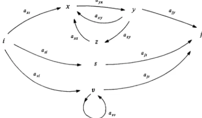
An example should clarify this point. Fig. 4 reproduces the elementary path and adjacent circuits explored in Fig. 3 and adds two other elementary paths with the same origin i and destinationj, i.e. (i, s,j) and (i, v,j).

ayx ax xz aY1 z asi a. is S \a q ajv / V

Fig. 4. Network of elementary paths and adjacent circuits linking poles i and j.

In the above example, it is clear that path (i, s,j) is an elementary path without any adjacent circuit while path (i, v,j) contains one loop centred on v. For simplicity, we can refer to these last two paths as 2 and 3, respectively - the initial path being referred to as I.

*j) = _maji = J(, x, v, j) + I(0, X, j) + Io, v, j)

- '(i-X)1 + '(i+)2 + I(N j)3

D

I( M)l + ai ajs + (aVi ajv) (i - a.)1

I984] STRUCTURAL PATH ANALYSIS 123

Note that in the case of the second path, the multiplier is one since the path has no adjacent circuits. Thus, in general, the global influence linking any two poles of a structure can be decomposed into a series of total influences transmitted along each and all elementary paths spanning i andj, i.e.

n n

i,-)j) = _{maji = I I(t> ) = E I8.jD MP)} (22)

p=l p=n

where p stands for elementary paths I, 2, k, ..., n. This decomposition is more

formally derived in the appendix where the relevant determinantal expansions are identified and related to path analysis interpretation.

IV. STRUCTURAL PATH ANALYSIS APPLIED TO

SOUTH-KOREAN SAM

In order to illustrate the usefulness and the types of questions which path analysis can answer, it is applied in the present section to the South-Korean SAM structure presented in Section If. Given the questionable nature of some of the estimates which went into the SAM, this application should be considered as a demonstration exercise of the types of results which can be obtained with this

approach.

It can be seen from Table 3 which gives the (truncated) matrix of average propensities (An) that the endogenous part of the matrix consists of 59 poles

(15 classes of factors, 15 classes of households and 29 production activities). There exists in such a structure a multitude of elementary paths.' One way of limiting the scope of the analysis is to study only those paths the length (i.e. number of arcs) of which does not exceed three. The more arcs a path contains, the weaker will be the direct and total influences transmitted along it.2

Even by limiting the scope of investigation in this fashion, this leaves many elementary paths which are not explicitly studied. Clearly the choice of paths to be explored depends on the questions raised. In what follows, we shall attempt to give a few selected examples organized according to (a) the SAM account in which the pole of origin is located and the SAM account containing the pole of destination; and (b) the type of question path analysis is supposed to elucidate.

Before actually embarking on the empirical analysis, it should be noted that the selected pole of origin (and its injection) within a SAM structure can be in any of the three endogenous accounts, production activities, factors, and insti- tutions. However, the triangular interrelationship of the endogenous structure of the SAM means that an elementary path must always travel in the triangular direction as shown on Fig. I. For example, if the injection occurs in a given

production activity, all elementary paths originating with that activity would

1 _{For example, in the structure represented by the i966 French input-output table disaggregated in}

only six sectors, Lantner (1974, p. 257), has identified 844 elementary paths.

2 One example suffices to illustrate this point: assume a path of length 4 (i.e. four consecutive arcs)

and the intensity of the influence between any two poles equal to o 5, then the direct influence would

be equal to (o05)4 or only o-o625. Experimenting with the SAM South-Korea data set revealed that it is

extremely rare to find a path of length four or longer transporting more than one half of a percent of the global influence transmitted from the pole of origin to the pole of destination. In any case, should such a path be presumed important, it could easily be identified by the computer.

124 THE ECONOMIC JOURNAL [MARCH

affect, first, other production activities (through the induced demand for inter- mediate inputs represented by the I-0 matrix A33) and factor demand (through the distribution of the value added among factors, i.e. matrix A13) before the influence is transmitted to institutions (in particular, the households) through matrix A21. Next in this sequence, transfers among institutions would be captured through A22 before the final link back to production activities (reflecting the consumption pattern of institutions, i.e. A32) can take place. Thus, there is an immutable ordering which is predetermined by the structure of the SAM. No elementary path can have arcs linking production activities directly to insti- tutions (the A23 matrix is empty) or linking the latter directly to factors (A12 is, likewise, empty).

The examples which were used below have, in common, that the injection in each case takes place in one of the production activities except for the last one which originates with households. In principle, any other pole of origin - among factors or institutions - could equally as well have been selected. In order to

provide a good basis for comparing the two types of multiplier decomposition structural path analysis is applied to the same eleven cases which were explored previously in Section II (see Table 4). These eleven different cases are analysed in Table 5. Each case (i) takes a given pole of origin (i) and destination (j) and measures the corresponding global influence; (ii) identifies the more important elementary paths spanning these two poles and measures their direct and total influences, respectively; and (iii) gives the proportion of the global influence between i andj transmitted through each specific path p.

These eleven cases can be, furthermore, broken down according to whether the pole of destination is a production activity, a factor or a household. Hence, these cases can be distinguished according to whether influence is transmitted

(i) from production activity to production activity (Cases I and II); (2) from

production activity to factors (Cases III-VIII); (3) from production activity to households (Cases IX and X); (4) from households to production activities

(Case XI); and (5) through path multipliers.

1. Influence of Production Activities on Other Production Activities

It should be noted at the outset that the present structural path analysis applied to a SAM does not yield the same results as applied to only the input-output matrix. In a SAM-type framework, a production activity can influence another one through the intermediate effects on factors and institutions (households) which are considered exogenous in the input-output framework.'

Case I in Table 5 explores the path analysis from an injection into the con- struction sector to its effects on mining. From the matrix of accounting multipliers, the global influence can be obtained-i.e. an injection of I,ooo Won into the construction industry yields an increase of 68 Won in the output of mining products (see column 3). The path analysis which is undertaken shows that only

25 1% (Column 8) of this additional production is caused directly by the demand for mining inputs by the construction sector through the elementary path (in this case, an arc) linking the two sectors without any intermediate poles.