Cell fate reprogramming using transcription factor feedback overexpression

Cell fate reprogramming using transcription factor

feedback overexpression

by

Nithin Senthur Kumar

Submitted to the Department of Mechanical Engineering

in partial fulfillment of the requirements for the degree of

Mechanical Engineer's Degree

at the

MASSACHUSETTS INSTITUTE OF TECHNOLOGY

June 2018

@

Massachusetts Institute of Technology 2018. All rights reserved.

Author ...

I

Signature

redacted

Department of Mechanical Engineering

May 11, 2018

redacted

Certified by...

Domitilla Del Vecchio

Professor

Thesis Supervisor

Signature redacted

A ccepted by ...

...

Rohan Abeyaratne

Chairman, Department Committee on Graduate Theses

MASSACHUSEUTS INSTITUTE

OF TECHNOLOGY

JUN 2

5

2018

LIBRARIES

MITLibraries

77 Massachusetts Avenue Cambridge, MA 02139 http://Iibraries.mit.edu/ask

DISCLAIMER NOTICE

Due to the condition of the original material, there are unavoidable

flaws in this reproduction. We have made every effort possible to

provide you with the best copy available.

Thank you.

The images contained in this document are of the

best quality available.

Cell fate reprogramming using transcription factor feedback

overexpression

by

Nithin Senthur Kumar

Submitted to the Department of Mechanical Engineering on May 14, 2018, in partial fulfillment of the

requirements for the degree of Mechanical Engineer's Degree

Abstract

Recent advances in stem cell research has demonstrated that the fate of a terminally differentiated cell can be reverted back to pluripotency. The ability to reprogram a differentiated cell back to its undifferentiated, pluripotent state would be a signif-icant breakthrough for regenerative medicine. For example, lost or damaged cells could be replaced by patient-specific reprogrammed cells, thus providing on-demand, compatible, high-quality cells of any required type. However, current protocols for reprogramming rely on simplified models that do not wholly capture system dynamics and on inefficient transcription factor overexpression. We study a gene regulatory net-work that determines the cell fate in the hematopoietic lineage and demonstrate that a deterministic model cannot capture the experimentally observed system dynamics. We also propose the use of feedback control to address inefficient reprogramming and implement two configurations of the controller on both deterministic and stochastic models of the Oct4-Nanog network. We also address practical issues such as place-ment of the regulator and consider the effect of inducing or constitutively producing microRNA on the protein steady-state distribution.

Thesis Supervisor: Domitilla Del Vecchio Title: Professor

Contents

1 Introduction

2 Modeling hematopoietic cell fate determination 2.1 Background ... . . . .. . . . . 2.2 Modeling assumptions for the PU.1 vs GATA-1 GRN 2.3 M odeling primer . . . .

Model reactions . . . Deterministic Model Conclusions . . . . .

3 Feedback overexpression to reprogram the Oct4-Nanog 3.1 Background . . . . 3.2 Endogenous system model . . . . 3.3 Controller dynamics . . . . 3.4 Multiplicity of infection . . . . 3.5 Modeling cell-cell variability using Poisson parameter . . 3.6 Regulator dynamics . . . . 3.6.1 Regulator model . . . .

3.7 MicroRNA dynamics . . . .

GRN

3.7.1 Comparison of CV for models with constitutive and no microRNA 3.7.2 Comparison of CV for models with constitutive, inducible, and

no m icroRNA . . . . 3.7.3 Realistic parameter values . . . . 2.4 2.5 2.6 13 15 15 18 20 22 24 25 27 27 29 30 38 40 42 42 53 55 58 59

List of Figures

2-1 HSC lineage tree studied in [9]. In this study, we will discuss the lineage determinant GRN of the Common Myeloid Progenitor (CMP) as it differentiates to either the Megakaryocyte-Erythroid Progenitor (MEP) or the Granulocyte-Macrophage Progenitor (GMP). . . . . 16 2-2 PU.1-GATA-1 GRN demonstrating self-activation and mutual repression. 18 2-3 Self-activating protein. . . . . 22 2-4 Promoter states: (a) po representing leaky production, (b) pi with

self-activated production, and (c) P2 when the promoter is fully repressed. 24

3-1 Waddington's view of cell differentiation [46]. A: Normal development consists of a pluripotent or multipotent progenitor cell differentiating to a differentiated cell state naturally. B: Reprogramming consists of forcing a differentiated cell up the landscape to its pluripotent state. C: Transdifferentiation consists of directly reprogramming a cell to a different state without intermediary reprogramming to the pluripotent

state... ... 28

3-2 Nanog-Oct4 GRN showing transcriptional interactions between the TFs [12]. u1 and U2 are the inducers for Nanog and Oct4, respectively. 30

3-3 Nanog (top) and Oct4 (bottom) transfer curves, representing the sta-ble steady states accessista-ble for each inducer level (u, or U2). . . . . . 31

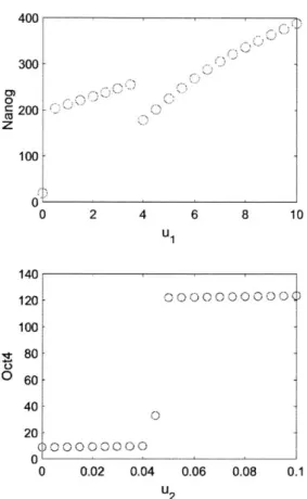
3-4 Nanog (top) and Oct4 (bottom) transfer curves, representing the sta-ble steady state that the system converges to when initialized at 0. . 32

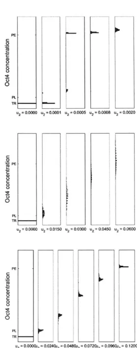
3-5 Distribution of steady-state Oct4 concentration in cells as a function of Oct4 inducer overexpression for top: no microRNA, middle: en-dogenous Nanog and Oct4 mRNA degradation bottom: enen-dogenous and synthetic Nanog and Oct4 mRNA degradation. The steady-state vales of the tristable endogenous systems are also shown (TR = tro-phectoderm, PL = pluripotent, PE = primitive endoderm). N=500,

M O I= 10. . . . . 43 3-6 Schematic of regulator and inducer used to control expression of

syn-thetic Oct4. Regulator and Oct4 on same (top) and different (bottom)

vector. ... ... 44

3-7 CV ratio (2V/1V) for regulator dynamics as a function of MOI and inducer concentration (u). . . . . 48 3-8 Mean ratio (2V/1V) for regulator dynamics as a function of MOI and

inducer concentration (u). . . . . 49 3-9 Comparison of pmfs for regulator models on 1V vs 2V. We find that

the 1V model has a higher CV for the same mean but the difference between the CVs decreases for large MOI. . . . . 50 3-10 Oct4 steady-state as a function of no, ni used to determine copy

num-bers of the regulator and synthetic gene vectors yielding the same mean. 51 3-11 Analytic pmf of steady-state Oct4 distribution for 2V for various

com-binations of regulator (no) and Oct4 gene (ni). Top: For roughly the same mean, we find the CV for the yellow curve with no = 2 to be roughly twice that of distributions with intermediate MOI. Bottom: CV is not as sensitive to low Oct4 vector MOI (blue) compared to regulator vector MOI (yellow). . . . . 52 3-12 CV for Poisson random variables n and n2

as a function of its parameter (M O I) . . . .

3-13 Comparison of analytical pmfs of Oct4 mRNA steady-state distribu-tion for models with constitutive microRNA (top row) and without microRNA (bottom row). The CVs and mean are shown for each distributions and we compare the two models having the same mean (column by column comparison). We find that there are parametric regions where the CV for the constitutive microRNA case is larger than that of the CV for the model without microRNA. . . . . 56 3-14 mRNA steady-state as a function of n for Km = 10 demonstrating the

offset ramp function form. . . . . 57 3-15 mRNA steady-state as a function of n for Km = 105 demonstrating a

smoother, monotonically increasing function. . . . . 57 3-16 Analytical pmfs of models with no microRNA (left), constitutive (middle),

Chapter 1

Introduction

There have been several recent advances in the stem cell field, with demonstrations that the fate of a terminally differentiated cell, contrary to what was traditionally believed, could be reverted back to pluripotency or directly converted to other dif-ferentiated cell types. The ability to "reprogram" a difdif-ferentiated cell back to its undifferentiated, pluripotent state would be a significant breakthrough for regenera-tive medicine. For example, lost or damaged cells could be replaced by patient-specific reprogrammed cells, thus providing on-demand, compatible, high-quality cells of any required type. Current reprogramming protocols are largely based on prefixed expression of suitable transcription factors (TFs), with the rationale that this over-expression could trigger transitions among the states of the gene regulatory networks (GRNs) that take part in cell fate determination. Yet, despite a decade of remarkable progress, the efficiency of these protocols remains low and the quality of produced cells is often unsatisfactory. These issues pose a formidable obstacle to the practical use of pluripotent stem cells.

A better understanding of the GRNs involved in this reprogramming process and tighter control of TFs could potentially alleviate the current bottleneck. My thesis work addresses both these factors: firstly, I studied and modeled one branch of the hematopoietic cell lineage and secondly, I modeled and simulated a feedback controller for better control of TF expression.

cell and hematopoietic cell fate is thought to be determined by a series of discrete, stable progenitor cells [42, 11, 311. Here we study the GRN of the first branching step of HSC differentiation to platelets, specifically the PU.1 vs GATA-1 network. Current deterministic models of this GRN do not predict experimentally observed multistablity and we demonstrate that stochasticity is necessary to explain this be-havior. A good understanding of this GRN is crucial for developing protocols that could provide an unlimited supply of safer and higher quality platelet transfusion product from human-induced pluripotent stem cells (hiPSCs). Platelet transfusions from donors are currently the most popular method of treating thrombocytopenia and other ailments that require an external platelet source. However, donor-derived platelets have side effects (hemolysis, infection) and logistic problems (short shelf-life). Using hiPSCs to directly produce platelets would address these issues, but a better understanding of the GRN is required to guide an effective protocol.

We also seek to improve current reprogramming protocols that rely on TF overex-pression by considering closed-loop feedback overexoverex-pression. This study is performed on the Oct4-Nanog GRN, which is a subset of the Yamanaka factors (Oct4, Sox2, Klf4, c-Myc) that have been shown to reprogram fibroblasts to pluripotency. We created deterministic and stochastic models that incorporate regulator dynamics and cell-cell variability. Simulation results demonstrate the efficacy of feedback control compared to open-loop overexpression. The stochastic model was also used to opti-mize the placement of the regulator gene and the type of expression (constitutive vs inducible) of microRNA. This approach is novel and could replace current prefixed overexpression protocols, leading to a fundamental shift in current cell fate repro-gramming strategies.

Chapter 2

Modeling hematopoietic cell fate

determination

2.1

Background

All mature, specialized blood cells have been shown to be derived from hematopoi-etic stem cells (HSCs) through a differentiation process called hematopoiesis [5, 401. Though there is currently no consensus on the mechanism that guides this pro-cess, there is evidence supporting that hematopoiesis occurs in discrete steps where each step is determined by the relative levels of certain transcription factors (TFs) [42, 11, 31]. A stochastic increase in the relative expression level of one TF over an-other at a cell lineage junction leads the differentiating cell down that corresponding lineage [37, 26, 44]. A diagram of the hematopoietic cell lineage with multipotent progenitor and specialized cells is shown in Fig. 2-1. HSCs have also been shown to self-renew, meaning they not only give rise to all blood cell types, but also have the ability to give rise to HSCs themselves without the need for differentiation, in a pro-cess called maintenance. HSC transplants from bone marrows of healthy donors are currently used in treatments of immune system disorders and some cancers because of these two properties.

A good understanding of the gene regulatory network (GRN) that governs hematopoiesis is critical to developing a model that can accurately predict the resulting specialized

HSC CI MPP LMPP CMP A/00 CLP GMP MEP

CD4 CD8 B NK Mono Gran Ery Mega

Figure 2-1: HSC lineage tree studied in [9]. In this study, we will discuss the lineage determinant GRN of the Common Myeloid Progenitor (CMP) as it differentiates to ei-ther the Megakaryocyte-Erythroid Progenitor (MEP) or the Granulocyte-Macrophage Progenitor (GMP).

cell phenotype from an undifferentiated progenitor cell, subject to overexpression of certain TFs. Here we study the GRN at the Common Myeloid Progenitor (CMP) state, at which point the cell can either differentiate to the Megakaryocyte-Erythroid Progenitor (MEP) or the Granulocyte-Macrophage Progenitor (GMP). Commitment to the MEP or GMP phenotype results in the differentiation to the erythroid or myeloid/lymphoid lineages, respectively [35]. Commitment to the MEP lineage re-sults in the production of megakaryocytes, which shed into platelets.

Platelets are a component of blood that are primarily used to stop bleeding by aggregating and clotting blood vessel injuries and are also responsible for vascular integrity, immunity, and neoangiogenesis (formation of new blood vessels). Platelet transfusions from donors are currently the most popular method of treating thrombo-cytopenia and other ailments that require an external platelet source. In the US alone, over 2 million platelet doses are transfused every year [1]. However, donor-derived platelets have major potential side effects including hemolysis, infection, sepsis, aller-gic reactions, and graft-vs-host diseases [431. Furthermore, platelets must be stored at room temperature; cooling them causes them to lose their clotting ability.

How-ever, room temperature storage increases the risk of bacterial infection leading to a shelf life of just a few days and so donors are continuously being sought to renew supplies that often go to waste. An alternative is to produce platelets directly from human-induced pluripotent stem cells (hiPSCs) derived from universal donor type platelets. The advantage of this method is that hiPSCs, like HSCs, have the ability to self-renew, and so once a colony of hiPSCs is grown, they can, in theory, be allowed to proliferate without a need to replenish their supply. Secondly, since these hiPSCs would be obtained from universal donor type platelets, there would be no issue with infections or graft-vs-host diseases that need to be considered when using current platelet transfusions. Lastly, this could potentially provide an unlimited supply of safer and higher quality platelet transfusion, if there were a protocol to force the hiP-SCs to differentiate into platelets (as opposed to other specialized blood cells). Here we study the GRN that governs the differentiation of the HSC or hiPSC at the CMP state into either MEP and GMP.

Literature indicates that the TFs PU.1 and GATA-1 regulate the differentiating HSC into either the myeloid/lymphoid or erythroid lineages, respectively [54, 33]. These 2 TFs have been shown to transcriptionally self-activate and interact antago-nistically [54, 33, 531 as pictorially depicted in Fig. 2-2. Arrows and blunt-end arrows represent transcriptional activation and repression, respectively. The expression level of GATA-1 has been shown to increase down the hematopoietic lineage from HSCs to MEPs and the TF is a key regulator of erythroid genes [8, 31. Similarly, PU.1 ex-pression increases as cells differentiate to the myeloid/lymphoid lineage [35] and has been shown to be critical for myeloid cell regulation. Early progenitor cells around the CMP stage have been shown to have relatively low levels of GATA-1 and PU.1 compared to more differentiated cells [3, 23J. A stochastically-driven increase in the concentration of either PU.1 or GATA-1 may perturb this balance and tip lineage commitment to either myelopoiesis or erythropoiesis [53, 13].

The PU.1-GATA-1 network has been extensively studied since the early 2000s [54, 33, 53]. Previous models of the PU.1-GATA-1 GRN in the literature make as-sumptions on the biological interaction between the TFs to explain the biologically

---Figure 2-2: PU.1-GATA-1 GRN demonstrating self-activation and mutual repression. expected bistable property of this GRN, in which one stable state corresponds to high levels of GATA-1 and low levels of PU.1 and vice-versa. However, some of these assumptions have not been experimentally validated. Specifically, the studies in [41] and [221 assume high cooperativity of TFs (n=2 and 4, respectively), though mutual repression and self-activation have been shown to occur primarily in their monomeric form [20, 10, 54]. The model presented in [61 introduces a hypothetical protein X that transcriptionally represses PU.1 and is activated by GATA-1, which has not been ex-perimentally identified. The model studied in [48] assumes both TFs can directly bind to each others' promoter sites and transcriptionally repress each other but this has not been shown. In this paper, we consider a set of biomolecular reactions for the system, in which none of these assumptions are made. Interestingly, we mathemati-cally demonstrate that the corresponding ODE model is monostable, which does not agree with experimental results demonstrating that the network should be capable of exhibiting two phenotypes, high GATA-1, low PU.1 (MEP) and low GATA-1, high PU.1 (GMP).

2.2

Modeling assumptions for the PU.1 vs GATA-1

GRN

The list of modeling assumptions (and evidence) used to derive the deterministic model are:

" PU.1 and GATA-1 transcriptionally self-activate their respective production [36, 341.

* PU.1 represses 1 production by binding to the complex formed by GATA-1 and its promoter. This complex forms repressive chromatin structure

effec-tively silencing transcription (the PU.1-GATA-1 complex has been shown to be present at repressed GATA-1 target genes) [45, 28].

" Similarly, GATA-1 represses production of PU.1 by binding to it on its target genes and prevents the recruitment of co-activators (such as cJun), which are critical for PU.1-mediated transcriptional activation 128, 541.

" PU.1 cannot directly bind to the GATA-1 promoter. [54] reports that PU.1 blocks GATA-1 activation without affecting GATA-1 mRNA, protein expres-sion, or nuclear translocation.

" GATA-1 cannot directly bind to the PU.1 promoter. [71 reports two GATA-1 binding sites on the PU.1 locus, a -18 kb site, which has not been shown to have a functional regulatory role, and a -17 bp site that potentially transcriptionally represses PU.1 production. However, [361 reports that the -14 kb PU.1 URE (to which GATA-1 cannot directly bind) is significantly more critical than the proximal promoter (which includes the -17 bp GATA-1 binding site) in myeloid cell line 416B for PU.1 expression. Therefore, here we only consider the con-tribution of the PU.1 URE (either activation or repression when bound with

GATA-1).

" All TF interaction occurs in their monomeric form. ETS TFs, such as PU.1 typ-ically bind as monomers (both to DNA and other proteins) [20]. Though there is evidence of GATA-1 dimerization [10], it exists primarily in its monomeric form. In particular, GATA-1 self-activation and binding to PU.1 occurs only in its monomeric form [10, 54].

" The promoters of both TFs are leaky [36, 34].

" Protein production occurs in a one-step process (no intermediary mRNA dy-namics).

2.3

Modeling primer

Here we demonstrate an example of how to model biochemical reactions using mass action kinetics. Consider the following reaction where two species, A and B interact to form species C at a forward rate a and reverse rate d:

A + B ,a ' kC (2.1)

d

The most common model for reaction networks is a deterministic model [17]. It assigns to each species a state variable corresponding to its concentration. The time-evolution of a species' concentration is given by an ordinary differential equation (ODE). Mass action kinetics dictates that the rate of a chemical reaction is proportional to the product of the concentrations of the reactants. Therefore, the dynamics of this system is given by:

A

= dC - aAB, (2.3)

= aAB - dC. (2.4)

Several TFs have been shown to transcriptionally activate or repress the production of other TFs by interacting with the promoter sites of the target TFs. Activation occurs when the complex formed by the TF and the promoter increases the transcription rate of the target TF. Conversely, repression occurs when the previous complex silences transcription. When modeling the concentration of promoters in their on or off states, we typically assume that DNA is conserved (i.e., the total promoter concentration is constant). Consider protein A that transcriptionally activates itself as shown in Fig. 2-3. Let the unbound promoter be represented by P0 and the protein A and promoter

total number of promoter sites. The reactions for this system are given below:

P, + A',\ P1, (2.5)

d

P1 -÷P, +A, (2.6)

A >0. (2.7)

Equation 2.5 refers to reversible reaction formed by the unbound promoter P and protein A to form P1. Equation 2.6 describes the production of protein A. Note

that here we model this as one-step protein production, but protein is generally produced from messenger RNA (mRNA) in a process called translation, which is in turn produced from the gene, in a process called transcription. Equation 2.7 refers to dilution of protein A. Since cells grow and their volumes increase, a species with a constant number of molecules decreases in concentration. This is modeled with a dilution term. The ODEs that describe this system are given below:

A=

Po = dP - aAPo, (2.9)

1 = aAPo - dP. (2.10)

We are often concerned with reducing the dimension of our ODE model. Since protein dynamics are significantly slower than binding reactions [4], we can reduce this system to a single ODE that describes the dynamics of A. Using the conservation of DNA,

Figure 2-3: Self-activating protein.

we can calculate the steady-state values of PO and P1.

PO + P1 =.PT, (2.11) P, = dAPO (2.12) a dA +

P

+

This leads to the dynamics of A given by:

Al=

aP- 6 A. (2.16)

1 + A/Kd

We note the Hill function form of the activation term ( Al). This indicates that for A/lKd << 1, we operate in a linear regime where the activation term is roughly aPTA

If there is a lot of protein A in the system, we find that the Hill function saturates

(lKd 1) and the activation term approaches aPT. In this regime, additional A does not increase its production rate since its promoter is saturated.

2.4

Model reactions

In this section, we use the same modeling principles in Section 2.3 on the biological system described in Section 2.2. The reactions that describe this system are given

below. Here po, shown in Fig. 2-4(a), and go are the unbound promoters of TFs PU.1 (P) and GATA-1 (G): Po+ P , Pi, (2.17) do go + G , g1, (2.18) do a, pi + G P2, (2.19) di g1 + P ,al g2, (2.20) di Po Po + P, (2.21) go

-n-

g

g

The reversible binding reactions between the unbound promoters (po and go) and their TFs (P and G) to form complexes pi (shown in Fig. 2-4(b)) and gj, respectively are given by (2.17)-(2.18). Reactions (2.19)-(2.20) describe the formation of complexes

P2 and g2 by reversible binding of G(P) with p1(g1), respectively. These complexes

represent the "off" state of the promoter wherein the gene is silenced as shown in Fig. 2-4(c) for P2. Reactions (2.21) and (2.22) describe the leaky promoter one-step production of P and G with rates apo and ago, respectively. P(G) is produced at rate

api(agi) _{when it is bound to its promoter as shown in reactions (2.23)-(2.24). Lastly,}

reactions (2.25)-(2.26) describe the decay of both transcription factors. Since the genes are self-activating, we have apo < api and ago < a,. To simplify the model,

(a) (b) (c)

Figure 2-4: Promoter states: (a) po representing leaky production, (b) pi with self-activated production, and (c) P2 _{when the promoter is fully repressed.}

2.5

Deterministic Model

Using mass action kinetics, the ODEs that describe this system are given below:

P = apip1 - 6pP + dop1 - aopoP + d1g2 - a1g1P, (2.27) S= ayg1 - 6GG

+

o = d'gi - a'goG, (2.29)

yi = aogoG - d'g₁ + d₁g2 - alg1P, (2.30)

92= aig1P - dig2, (2.31)

Po = dop1 - aopoP (2.32)

P1 = aopoP - dop1 + d'1p2 - alp G, (2.33)

P2 = a' p1G - d'P2. (2.34)

Here we once again use the conservation of DNA given by:

PO +PI +P2 =PT, (2.35)

Once again using the fact that protein dynamics occurs on a slower scale than binding reactions, we obtain the reduced model describing the dynamics of PU.1 and GATA-1.

apoPT + K p P + + PG JPP (2.37) Kd KdKd1 * 'g09T + C G =Kd G -6GG, (2.38) 1+ I+ _{Kd KdKd} PG _ _{K l}G

The number of steady states of this reduced system is the same as the number of steady states in the original network. Setting the derivatives to zero and performing algebraic manipulations results in a quintic equation. It is not easy to show directly that this equation has a unique solution for all possible choices of kinetic parameters. Thus, in order to determine the number of positive equilibria, we use the advanced deficiency algorithm developed in [14, 16, 24], and implemented in the "Chemical Reaction Network" toolbox [151. When the algorithm is applied to our network, it shows that it cannot admit multiple positive equilibria for any combination of kinetic parameters. Hence, the deterministic model cannot explain the bistable behaviour observed experimentally [35, 8, 3].

2.6

Conclusions

Deterministic models are usually justified under the assumptions of sufficiently large volume and sufficiently large number of molecules [27], or, under some conditions such as fast promoter kinetics [251. In such cases, an ODE model captures the system's dynamics, and it produces a similar qualitative behaviour to the one produced by the stochastic model. However, these assumptions are not usually satisfied in practice due to the fact that cell-fate GRNs have usually very low gene copy numbers. Fur-thermore, in such cells, transcriptional regulation is often mediated by an additional regulation layer dictated by DNA methylation and histone modifications, commonly referred to as chromatin dynamics. For example, the presence of nucleosomes makes binding sites less accessible to TFs and therefore TF-gene binding/ unbinding is

modu-lated by the stochastic process of chromatin opening [38, 30, 501. Several experiments have confirmed the role of the aforementioned complex transcription processes in slow promoter kinetics [39, 49, 29, 521. Therefore, the qualitative behaviour produced by deterministic models can be erroneous. We are currently preparing a paper that con-siders the stochastic version of this chemical network and analytically construct the stationary distribution to show that this distribution is indeed capable of admitting a multiplicity of modes.

Chapter 3

Feedback overexpression to

reprogram the

Oct4-Nanog

GRN

3.1

Background

The state of a multistable gene regulatory network (GRN) can be determined by the concentration of the transcription factors (TFs) that make up the network. Wadding-ton's view of cell differentiation [51] consists of cells, represented by balls, that roll down a landscape of bifurcating valleys as shown in Fig. 3-1. Each valley represents a possible cell fate and the ridges between the valleys maintain the cell fate once it has been chosen. A cell in its pluripotent state occupies the top of this landscape. Normal development consists of a pluripotent or multipotent progenitor cell differ-entiating to a committed cell state naturally over time. Reprogramming consists of forcing a differentiated cell up the landscape to its pluripotent state. Transdifferentia-tion consists of directly reprogramming a cell to a different state without intermediary reprogramming to the pluripotent state.

According to Waddington, each stable state of a GRN can be represented by a particular cell phenotype and the transitions between the phenotypes are triggered by external stimuli or noise. Our ability to trigger these transitions is dependent upon how well we can artificially stimulate the GRN [21]. The current method of triggering changes in cell phenotypes is by overepxressing certain TFs above their endogenous

C

Normal development Reprogramming to pluripotency Direct reprogramming (Dedifferentiation) (Transdifferentiation) Key

*

*

Figure 3-1: Waddington's view of cell differentiation [46]. A: Normal development consists of a pluripotent or multipotent progenitor cell differentiating to a differenti-ated cell state naturally. B: Reprogramming consists of forcing a differentidifferenti-ated cell up the landscape to its pluripotent state. C: Transdifferentiation consists of directly reprogramming a cell to a different state without intermediary reprogramming to the pluripotent state.

level [18]. Here "endogenous" refers to the cell's natural GRN without any artificial modifications. However, the success rate of protocols that rely on overexpression remains low and once an experiment begins, the TF levels cannot be adjusted [32]. [12] suggests that the low reprogramming efficiency from TF overexpression is be-cause there is no general guarantee that a GRN's dynamics will allow transitions to a desired target state under the imposed stimuli. Here we propose a method for artifi-cially enabling transitions between stable states that does not depend on the natural network's dynamics and would allow for more efficient reprogramming.

The goal of this project is to reprogram fibroblasts to efficiently generate high qual-ity human-induced pluripotent stem cells (hiPSCs) by using feedback overexpression of certain TFs, in particular Oct4, Sox2, Klf4, and c-Myc (OSKM factors). These 4 OSKM TFs have been shown to induce reprogramming to iPSCs from fibroblasts [47]. Here we study a model of the Oct4-Nanog GRN and develop a feedback controller to arbitrarily place the steady-state of Oct4 and Nanog. The purpose of using models is to address questions regarding the optimization of virus construction and to study how various parameters affect the distribution.

3.2

Endogenous system model

We began this analysis using a tristable network incorporating the Nanog-Oct4 GRN, developed in [121 and pictorially represented in Fig. 3-2. Arrows represent transcrip-tional activation and blunt-end arrows represent transcriptranscrip-tional repression. The ex-ogenous inputs ui and U2 in Fig. 3-2 are the synthetic signals that directly increase the concentration of Nanog and Oct4, respectively. The list of reactions for this GRN is given in [12] and the coupled ODEs that describe the dynamics endogenous network with the exogenous inputs are given below (O=Oct4, N=Nanog):

K aOoo + oi(+) 2 + a2(N )2 + a03( )2

O6=1 + ( + (L)2 + (NO ()2 )2 + u2 - 0 (3.1) 01 101lk2 ok₀₂ = Ho+ u 2 - 7O, (3.2) 60 K NO + aNl(k )2 + ckN2(

)

aN3

N

+

]

where the Hill function terms for Oct4 and Nanog are represented by HO and HN,

respectively. The above system is tristable and the three stable equilibrium points cor-responds to the trophectoderm (TR), the desired pluripotent state (PL), and primitive endoderm (PE). Fig. 3-3 plots the transfer curves for Nanog and Oct4, which show the stable steady states for each level of inducer concentration. Since the addition of inducer to the system changes the GRN's dynamics, the steady states themselves change. Both the Nanog and Oct4 transfer curves demonstrate that the PE state is accessible for all inducer values and that the TR and PL states are only accessible for sufficiently low inducer concentration. Furthermore, note that the PE state represents the high steady state for Oct4 but is intermediate in terms of Nanog expression (there is no requirement for a steady-state to have the same relative expression levels of all TFs in the GRN). Also note the disparity in the change of inducer for the system to have multiple steady states to switch to a single steady state. For u1 (Nanog

overex-Figure 3-2: Nanog-Oct4 GRN showing transcriptional interactions between the TFs [12]. ui and u2 are the inducers for Nanog and Oct4, respectively.

pression), the TR state is lost for low inducer values and the PL state is attainable for a wide range of u1. However, the behavior of both TR and PL states are quite

similar for u2.

Fig. 3-4 plots the steady-state that a trajectory initialized at 0 converges to for a given inducer concentration. The single circle around 40 nM for Oct4 represents the PL state demonstrating that it would be extremely difficult to guide the system to pluripotency if one were to use U2 to control the system.

3.3

Controller dynamics

Here we propose the use of feedback control to arbitrarily place the steady-state of TFs, so that upon removal, the system converges to the desired steady-state. The reason we choose to not use direct overexpression is because we have shown that overexpressing Oct4 or Nanog may lead the system to overshoot and converge to the undesired PE state. Implementation of this feedback control requires the use of lentiviral constructs that are inserted into cells. These constructs are pieces of DNA that use cell machinery to produce proteins, which can act as input signals (activation or repression) for other processes in the host cell. Specifically, feedback overexpression involves using microRNA to degrade the mRNA of the TF we wish to control (high gain negative feedback) and overexpression of the same TF.

For simplicity, we will consider a bistable system of a protein X, that transcrip-tionally activates itself. We would like to control the concentration of X from its low state by feedback overexpression so that it is within the stability region of its high state and so once the controller is removed the endogenous system converges to the desired high state. Though for this toy system, overexpressing X sufficiently

4__ _ _ _-3 0 C 2 z 1C 14 12 10 C.) 0 4 2 -0 'TR 171 PE PE - P-L, 0 2 4 6 8 1 u8 0 - - -- ---- --- --0 0TR 0 - EPL PE 10 0-E0 L ].i-AL . . . .. 0 0.02 0.04 0.06 0.08 U 2 0 0.1

Figure 3-3: Nanog (top) and Oct4 (bottom) transfer curves, steady states accessible for each inducer level (u1 or U2).

representing the stable

400 300 CM 0 200 z 100 0 0 140 120 100 80 60-40 20 0 0 2 4 6 8 10 U 1 0.02 0.04 0.06 0.08 U 2 0.1

Figure 3-4: Nanog (top) and Oct4 (bottom) transfer curves, representing the stable steady state that the system converges to when initialized at 0.

k-I

C000000000(

0

will cause it to converge to its high state we use this model as an example on how to implement similar control for the Oc4-Nanog GRN.

The endogenous system is bistable and is initialized with its concentration in the stability region of the low state. The controller, which consists of the microRNA gene and synthetic x, gene with copy number no is introduced making the system monostable. We aim to arbitrarily place the concentration of the total TF in the sta-bility region of the high state by only controlling the production rate of the synthetic mRNA. Upon removal of the controller (setting the synthetic TF to 0), we hope to show that the steady-state value of the endogenous TF concentration approaches that of the high state.

The reactions describing this system are given below. Here xe is the endogenous gene that produces mRNA, me at a rate ao as shown in Equation 3.5. Equations 3.6 and 3.9 represent the production of X from me and m, respectively at rate K. The TF dimerizes (Equation 3.7) and binds to xe in Equation 3.10. Equation 3.8 describes the production of synthetic mRNA, m. Here since we have assumed that it is consti-tutively produced, we represent its production by the copy number of its DNA, which is no. Its rate of production is a, which is the input to the system. Here we assume that the promoter is inducible by an external inducer and that a is proportional to the inducer concentration. The microRNA, s is constitutively produced from a dif-ferent vector with copy number ni (Equation 3.14) and enzymatically degrades both synthetic and

endogenous

X xe * + Xe

+

,

+

0,

0,

0,

0,

0.

Xe = d* C1 - a*xe X2, he = ao Xe +

ai

+

a

d

a

d

a

+

I

Using conservation of DNA, Xe + C1 = XT we find the equilibrium value of the species

a2n 1 04 a mas d + 6c' ano MS = _, Xe = XT 1+ C1-Xe x x 2 XX2 KdI1 Xao + Cel (X 2) me () Kdl d Y2 1+ _{Kd IK7}

where

'Yi

+

(3.20) (3.21) (3.22) (3.23) (3.24) (3.25) (3.26) (3.27) (3.28) (3.29) (3.30) (3.31) (3.32) (3.33) (3.34) (3.35)

following reduced system:

XTK a + al X

2

Kno + _ )___ 6 Xx (3.36)

71 2 1 + Kd X

The first term in X is from the production of X by the controller (synthetic X) and the second term is Hill function representing the transcriptional endogenous activation

by X. We can rewrite this as:

K1

a

i +- H(X) - JxX (3.37)

Y1 7Y2

with constants K, ~ no, K2. Increasing the amount of microRNA and the synthetic

promoter strength corresponds to increasing n, and a, respectively because Y1, 7Y2 C1 + C2n1 for positive constants C1, C2. Therefore, for large ni1, a we have:

~ Kla - 6xX (3.38)

7Y1

and so Xieq ~K2. In order to drive X to a desired equilibrium point, we require a and n, sufficiently large and that a/71l becomes a non-zero constant. As a sanity check we can see if ni = 0, _Y1, Y2 = m and we recover the endogenous system with constitutive synthetic production. Now, if we remove the microRNA degradation of m. (remove Equation 3.12) so that the controller only degrades me, the X dynamics

are given by:

Kano _XTK / ₀ a₁X2

x = + ( ) KdK* _ -XX (3.39)

6m 7Y2 _{+ X',1}

Rewriting this as:

= K ₁a K<2

X= - H(X) - xX (3.40)

6m Y2

Here just increasing ni is sufficient to ensure that: Kla K ~ -6xX (3.41) 6m

and so Xleq ~ Kja, which is unique and controllable from a. Note here there is no

requirement for increasing a with Y1, Y2. Now, if we remove microRNA degradation

of me (remove equation 3.11), we would expect to not be able to control Xieq. The X dynamics are of the form:

K1

a

X

6xX

This matches our intuition since here we shut down the synthetic production of X by increasing both a and ni.

Applying the same controller reactions (for endogenous mRNA degradation only) to the endogenous Nanog-Oct4 network results in the following dynamics

o=

Go

S= N HN - KNUl -YNN. (3.44)

GN

The parameters, Go and GN are increasing functions of microRNA steady state and so for sufficiently large amount of microRNA, the endogenous network is shut down:

0 KoU2 - 7YO0, (3.45)

N KNui - _YNN. (3.46)

The steady-state of this system is linear with respect to the inputs u1, U2. For the

system with microRNA degradation of both endogenous and synthetic mRNA, the protein dynamics are of the form:

KO

0 ---

Ho +

-

y00,

(3.47)

Go Go

= _N HN + KNUl - 7NN. _(3.48)

GN GN

Here we note that for large microRNA degradation, the inputs a₁, U2 also need to be

From this analysis, it appears that the controller with endogenous mRNA degrada-tion has the benefit of not only being able to produce linear input-output system response but also requiring significantly less input than the system with degradation to both synthetic and endogenous mRNA. However, in reality, the vector copy number varies from cell to cell (i.e., not every cell will receive no copies of the synthetic gene) and so we need to address the robustness of this controller to this form of stochasticity.

3.4

Multiplicity of infection

The multiplicity of infection (MOI) is the ratio of the total number of infectious agents (e.g., lentiviruses with synthetic Oct4 and microRNA gene) to infection targets (e.g., cells). The protocol to infect a colony of cells with a desired MOI is given below

(adopted from [2]):

" Seed a fixed number of cells into each well (e.g. 75,000 cells in each well of a 6-well dish) by:

1. Diluting cells in media (e.g. dilute 525,000 cells into 14 mL of DME media) 2. Mixing well by pipetting/inverting

3. Adding 2 mL of cell suspension to each well (e.g. (2mL/14mL) x 525,000 cells = 75,000 cells)

" Incubate the cells overnight.

" If using freshly collected virus, use a filter to remove cells/debris. If using frozen virus, rapidly thaw in warm water bath. At this point the concentration of the virus stock is unknown.

" Prepare dilutions of virus (1:10, 1:100, 1:1000, etc.) in same DME media. " Add the viral dilution to each well of cells that were grown overnight and

" Calculate the percent of fluorescent-positive cells in each well (MOI). Only con-sider wells with <40% fluorescent-positive cells. Here we assume 1 integration event per cell because for >40% fluorescent-positive cells, we risk counting cells with multiple integration events per cell.

" Calculate the titer (transduction units/mL) of the original virus stock using the dilution factors (method 1) or virus volume (method 2).

1. Method 1: TU/mL = (Number of cells transduced x Percent fluorescent x Dilution Factor)/(Transduction Volume in mL). Method 1 example: If the 1:100 well has 25% fluorescent cells and 150,000 cells were originally transduced, then there are (150, 000 x 0.25 x 100)/(1.5 mL) = 2.5 x 106 TU/mL

2. Method 2: TU/mL = (Number of cells transduced x Percent fluores-cent)/(Virus volume in mL). Method 2 example: If 15 pL of virus is added to 150,000 cells resulted in 25% fluorescent cells, then there are

(150, 000 x 0.25)/(0.015 mL) = 2.5 x 106 TU/mL

3. For an accurate titer, take the average of multiple dilutions.

" Now that the titer is known, to get a desired MOI for a certain number of cells, pick the appropriate volume of the virus stock (e.g. say titer was calculated to be 105 TU/mL and we want MOI=10 for 100 cells, we need 105 TU so take 1 mL of virus stock and add it to plate of cells (volume of virus stock = MOI x cells/titer)).

The variation in vector copy number is modeled as a Poisson distribution with the multiplicity of infection (MOI) as the Poisson parameter. The intuitive reason for this is because if we had 100 balls (infectious particles) that are randomly thrown in 10 boxes (cells), the probability that a given box has n balls is Poisson with parameter 10.

3.5

Modeling cell-cell variability using Poisson

pa-rameter

A numerical study was performed with the vector copy number having a Poisson distribution. Initially, two configurations of the controller (for both Oct4 and Nanog) were studied: degradation of endogenous mRNA only and degradation of both en-dogenous and synthetic mRNA. For simplicity, we assume that the microRNA and TF genes are on the same vector with copy number n and we adjust the promoter strength of the microRNA to change the microRNA steady-state. We found that for sufficiently strong mRNA degradation, there is approximately a linear input-output relation between the inducer concentration and the mean of the protein distribution for both controllers as shown in the deterministic model. However, in the system with just endogenous mRNA degradation, the distribution widens as inducer concentration

increases. This occurs because the microRNA shuts down the endogenous network but there is no control of the variation in vector copy number of the synthetic gene as shown by the following dynamics:

=o Kou₂

0 = Ho + - -00, (3.49)

Go 6M

N = HN + KNU - NN. (3.50)

GN 6M

Once again Go, GN are increasing functions of the microRNA steady-state (for Oct4 and Nanog, respectively) and so the Oct4 steady-state is of the form:

0 = KO2, (3.51)

6,n60

= Cnu2, (3.52)

for some positive constant C. Here we find that the Oct4 steady-state (and Nanog) is proportional to the Poisson random variable n. In particular, there is no way to control for this variation from the input U2.

in copy number is accounted for leading to a tighter distribution. This is reflected in the system dynamics of the form:

O

=

K

+

Go Go

= N HN + KNUl -NN. (3.54)

GN GN

For large Go, GN, the Oct4 steady-state is given by:

0

Go~yo'

n U2 (3.56)

1+ na2' (-6

where a2 _{is the microRNA production rate and is assumed to be large. Therefore,}

the cost of degrading the synthetic mRNA is that the inducer concentration (u₁, u2)

needs to be significantly larger to produce any appreciable change in the Oct4 steady state value. Here the parameters, Go and GN are of the form C1 + C2n (C1, C2 > 0),

and KO and KN are of the form C3n (C3 > 0).

The Oct4 steady state concentration for a cell population (N=500) infected with a lentivirus (MOI=10) containing both the synthetic Oct4 gene and the microRNA gene as a function of inducer concentration (U2) is shown in Fig. 3-5. The left plot is the

open-loop case (no microRNA), the middle plot is for endogenous mRNA degradation only, and the right plot is for both endogenous and synthetic mRNA degradation. For no inducer, the distribution of all 3 plots indicate the cells are in the initial TR state. For the open-loop case, increasing the inducer slightly results in a small proportion of cells converging to the desired PL state (parameter values were chosen so that this population was roughly 1% of cells). Increasing the inducer concentration resulted in the cell population converging to the undesired PE state. For the system with endogenous mRNA degradation, there is a spreading out effect in cell population. This is because the Oct4 steady-state is a scaled version of a Poisson distribution, which only has probabilities associated for non-negative integers. The distribution of the model with degradation to both endogenous and synthetic mRNA retains the

input-output linear response of the mean but is significantly tighter.

3.6

Regulator dynamics

Until this point of analysis, the inducer was modeled to directly increase the Oct4 steady-state concentration without limit. This assumption was then relaxed to ac-commodate a more realistic model of gene activation. A regulator gene is also inserted in the lentivirus that produces a protein TetR, which dimerizes in the presence of the inducer (the true input to the system). The complex of 2 TetR molecules and 1 Dox molecule can bind to the promoter of and activate the synthetic Oct4 gene. Fig. 3-6 demonstrates the two experimental choices for where to place the regulator: on the same or different vector as the Oct4 gene. In the different vector case, the copy num-ber of the regulator vector is no and that of the Oct4 gene is n1. This was done to

answer if it was better to place the regulator and gene on the same (1V) or different vectors (2V).

3.6.1

Regulator model

Here we consider a toy model incorporating the regulator and inducer that produces synthetic Oct4 (i.e., no endogenous GRN). TetR (T) can dimerize only when bound to the inducer, Dox (D) and the resulting complex binds to the synthetic Oct4 pro-moter (Po). The activated propro-moter (P1) produces mRNA (m). For simplicity we

also assume no inducer dynamics and so binding to the promoter does not affect its concentration: this is reasonable if D is large and we are operating in a saturating inducer region (explained later). The reactions for the same vector configuration are

0 Pt-TIR u₂=0.0000 u₂ =0.0001 U2=0.0005 U=0.0008 u2 0.0020 0 8 U2= 0.00009 U2 0.04 U2 0.0 0 0.06 =2 0.0200 :PE 0 o L U2 =0.00O0.04(2 0.0U 2 0 0720 2 00450 j 006002

Figure 3-5: Distribution of steady-state Oct4 concentration in cells as a function of Oct4 inducer overexpression for top: no microRNA, middle: endogenous Nanog and Oct4 mRNA degradation bottom: endogenous and synthetic Nanog and Oct4 mRNA degradation-. The steady-state vales of the tristable endogenous systems are also shown (TR = trophectoderm, PL = pluripotent, PE = primitive endoderm). N=500, MOI=10.

Dox Tet Oct4

rI

---.----

Figure 3-6: Schematic of regulator and inducer used to control expression of synthetic Oct4. Regulator and Oct4 on same (top) and different (bottom) vector.

given below: n -% n + T, (3.57) T+D a C1, (3.58) d T+C1 + C2, (3.59) d C2 +

POa

0,

The ODEs that describe this system include:

O

01

Using conservation of DNA (PO + P1 = n) we can show (Kd = 4:

PO

C

P = n C2 K (3.76)

1 + C21Kd

For binding significantly faster than dilution (d >> 6), we can show the equilibria of

C2 and C1 as: C = D (3.77) Kd TO1 = T2D Kd K . (3.78) From Tq =T we find: a n2D 0q ( _{6 6} )n 2TD 6T 1 + n - (3.80) n1 +n2D (-0

For the case of different vectors the form of the equilibrium 0 is given by:

Oeq n1( _{1-F 2~}

)

I + noD

Here we note a difference from our previously assumed activation term given by:

O

In particular, activation is now a Hill function term and so for low inducer levels (noD << 1) it is linear, but after the promoter is saturated (nrD >> 1), increasing the inducer concentration does not change the Oct4 steady-state. To summarize, the dynamics for the two configurations in consideration are given (for the 1V case):

Dn 2

O

6 + Dn

-where n is the copy number of the vector. The 2V dynamics is given by: Dn 2

O

1 + Dno

where no and ni are the copy numbers of the regulator and Oct4 gene vectors, respec-tively. A configuration was deemed better if it had a smaller coefficient of variation

(CV) for a given mean and is given by:

CV(X)

E[X

E[X]

for a random variable X (in our case, it would be the steady-state value of Oct4). We simplified the analysis by assuming that the microRNA had completely shut down the endogenous network so we are only concerned with the steady-state distribution of the synthetically produced Oct4. The CV for the 1V model is calculated by assigning each probability of a Poisson distribution to the corresponding Oct4 steady-state. For example, let the Oct4 steady-state be a function,

f,