Dynamical downscaling with the fifth-generation Canadian
regional climate model (CRCM5) over the CORDEX Arctic
domain: effect of large-scale spectral nudging and of empirical
correction of sea-surface temperature
Maryam Takhsha1 · Oumarou Nikiéma1 · Philippe Lucas-Picher1 · René Laprise1 · Leticia Hernández-Díaz1 · Katja Winger1
Received: 27 February 2017 / Accepted: 12 September 2017 © The Author(s) 2017. This article is an open access publication
most notable positive effect over the Arctic is a reduction of the T2m bias over the North Pacific Ocean and the North Atlantic Ocean in all seasons. Future projections using this method are compared with the results obtained with the tra-ditional 2-step dynamical downscaling (CGCM-RCM) to assess the impact of correcting systematic biases of SST upon future-climate projections. The future projections are mostly similar for the two methods, except for precipitation.
Keywords Regional climate modelling · CRCM5 ·
CORDEX · Climate change projections · Arctic · Dynamical downscaling · SST bias correction
1 Introduction
Arctic regions have experienced amplified warming at twice the rate of the global average (ACIA 2004; IPCC 2013). Yet, as stated by Overland et al. (2014): “Arctic air tem-perature is both an indicator and a driver of regional and global changes”. Thus, the climate of the Arctic deserves getting attention due to its dual nature, with its response to global climate change and its important role in affecting global climate.
The Arctic sea ice has been in a sharp decline during the past decades. An average of 53,900 sq. km of Arctic sea ice loss per year is observed using satellites records (Ramsayer
2014). According to IPCC, the annual mean Arctic sea ice extent decreased over the period 1979–2012 with a rate of 3.5–4.1% per decade, and the decrease is more than three times larger (9.4–13.6%) for the summer sea ice minimum (IPCC 2013). The national snow and ice data center located in Colorado announced that Arctic sea ice extent in Septem-ber 2016 is recorded as the second lowest yearly minimum since satellites record beginning in 1978, with 4.14 million
Abstract As part of the CORDEX project, the
fifth-gener-ation Canadian Regional Climate Model (CRCM5) is used over the Arctic for climate simulations driven by reanalyses and by the MPI-ESM-MR coupled global climate model (CGCM) under the RCP8.5 scenario. The CRCM5 shows adequate skills capturing general features of mean sea level pressure (MSLP) for all seasons. Evaluating 2-m tempera-ture (T2m) and precipitation is more problematic, because of inconsistencies between observational reference datasets over the Arctic that suffer of a sparse distribution of weather stations. In our study, we additionally investigated the effect of large-scale spectral nudging (SN) on the hindcast simu-lation driven by reanalyses. The analysis shows that SN is effective in reducing the spring MSLP bias, but otherwise it has little impact. We have also conducted another experi-ment in which the CGCM-simulated sea-surface temperature (SST) is empirically corrected and used as lower boundary conditions over the ocean for an atmosphere-only global simulation (AGCM), which in turn provides the atmospheric lateral boundary conditions to drive the CRCM5 simula-tion. This approach, so-called 3-step approach of dynami-cal downsdynami-caling (CGCM-AGCM-RCM), which had con-siderably improved the CRCM5 historical simulations over Africa, exhibits reduced impact over the Arctic domain. The Electronic supplementary material The online version of this
article (doi:10.1007/s00382-017-3912-6) contains supplementary material, which is available to authorized users.
* Maryam Takhsha [email protected]
1 Département des sciences de la Terre et de l’atmosphère, Centre ESCER (Étude et la Simulation du Climat à l’Échelle Régionale), Université du Québec à Montréal (UQAM), Montreal, Canada
sq. km. The lowest Arctic sea ice extent was in September 2012 with 0.73 million sq. km lower than in 2016 (http:// nsidc.org/arcticseaicenews/).
Because of the vulnerability of the Arctic to climate changes and because of the pronounced and rapid changes that it is projected to undergo in the next decades, there has been a growing interest in performing future projections over this region. Overall, an increase in precipitation, large reduc-tions in sea ice and glacier volume, sea level rise and the thawing of permafrost are expected consequences in the Arc-tic of the projected global warming (IPCC 2013). Accord-ing to the Coupled Model Intercomparison Project phase 5 (CMIP5), Arctic sea-ice extent is projected to decrease by 94% in September of 2081–2100 compared to 1986–2005, resulting in a nearly ice-free Arctic Ocean, which will cause increase in wave heights and the duration of wave season (IPCC 2013).
From the side of regional climate modelling, a compre-hensive study of RCM hindcast simulations was done as a part of the Arctic Regional Climate Model Intercomparison Project (ARCMIP; Curry and Lynch 2002). It was found that the different treatment of orography and land-sea mask for each model caused a large scatter for 2-m temperature and consequently in downwelling radiation between models. The cloud cover also showed a large scatter between models due to the diversity of cloud modelling assumptions. Addition-ally, large internal variability for each RCM across the Arctic region (Rinke et al. 2004) leads to even more scatter between results (Rinke et al. 2006). Due to internal variability, each individual RCM simulation represents only one realization of the spectrum of plausible solutions. Rinke and Dethloff (2000) showed that the internal variability is more important in pan-Arctic simulations, especially during winter, because of the strong polar vortex that traps atmospheric waves in the domain for long periods of time, reducing the inflow of new LBC information.
The Arctic region is particularly challenging to regional climate modellers. The lack of reliable observational data-sets in the Arctic often makes it difficult to determine whether the differences between hindcast simulations and observations are really due to model biases or from inad-equate observational spatiotemporal coverage.
One of the issues for nested models over polar regions is the reduced control exerted by the lateral boundary con-ditions (LBC) upon the regional simulation (Rinke and Dethloff 2000), leading to large internal variability, as mentioned before. Large-scale spectral nudging technique (SN) enhances the control exerted by LBC (von Storch et al. 2000; Biner et al. 2000). The SN technique consists in constraining the RCM atmospheric large scales toward those of the driving data. This technique has shown to be effective in reducing substantially systematic biases that are present in some RCM simulations (e.g. Berg
et al. 2013; Glisan et al. 2013). Also, RCM subgrid-scale physical parameterizations have often been developed and optimised for mid-latitude climate, so non-native polar simulations may be expected to exhibit larger biases (e.g. Lucas-Picher et al. 2013).
On the other hand, it is well documented that nested RCMs inherit biases present in the driving data supplied as lateral BC in the atmosphere and lower BC over the oceans; these biases can be rather important when RCM are driven by CGCM-simulated data. All CGCMs exhibit systematic bias in sea surface temperature (SST) and sea-ice concentra-tions (SIC) (e.g. IPCC 2013). The resolutions of the ocean module in CGCMs are often too coarse to capture important regional oceanic processes such as the offshore transport of cool waters by mesoscale eddies or the sharp vertical temperature gradient (e.g. Richter 2015). Given the sensitiv-ity of RCMs simulations to the biases of the driving data, several attempts have been made to develop bias-correction methods, such as the studies of Christensen and Christensen (2007), Katzfey et al. (2009, 2011), Bruyère et al. (2014), Yu and Wang (2014), and Hernández-Díaz et al. (2016; herein-after HD16), to cite but a few.
Nevertheless, CGCMs simulations are the only avail-able data for driving RCM simulations of future climate. Dynamical downscaling of the CGCM projections over the Arctic by RCMs shows warming up to 6.5 K in the mean tropospheric temperature over Barents, Kara Seas and the Beaufort Sea during winter (Rinke and Dethloff 2008), the regions corresponding to the areas with the maximum pro-jected sea ice loss. Warming up to 15 K over the Arctic Ocean in autumn and winter is projected by the end of the century (Koenigk et al. 2015). Furthermore, studies agree in projection of a reduction of the sea-level pressure by the end of 2100 (Chapman and Walsh 2007; Rinke and Deth-loff 2008; IPCC 2013; Koenigk et al. 2015). Several models project an increasing in 2-m temperature (Keup-Thiel et al.
2006; Stendel et al. 2008; Førland et al. 2009; Rinke et al.
2012; Steiner et al. 2013) as well as an increment of precipi-tation (Stendel et al. 2008; Steiner et al. 2013; Zhang et al.
2016) by the end of the century.
The Arctic is also one of the recommended domains for the COordinated Regional climate Downscaling EXperi-ment (CORDEX), an international coordinated sets of experiments for hindcast, historical simulations and climate projections under RCP4.5 and RCP8.5. This framework is developed to evaluate, and possibly improve, RCMs and downscaling methods as well as to provide regional climate-change projections for impact and adaptation studies.
The Canadian Regional Climate Model, version 5 (CRCM5) has contributed to the CORDEX program over three CORDEX domains so far: North America (Martynov et al. 2013; Šeparović et al. 2013), Africa (Hernández-Díaz et al. 2013; Laprise et al. 2013) and South Asia (Alexandru
and Sushama 2014). Paquin and Sushama (2014) have car-ried some experiments with CRCM5 over the Arctic.
The aim of this study is to evaluate the performance of the CRCM5 over the Arctic domain following the COR-DEX protocol. Thereby, we investigate (1) the sensitivity of a hindcast simulation driven by the reanalyses to the appli-cation of SN and (2) the sensitivity of a historical simula-tion driven by the output of a GCM to the empirical correc-tion of systematic SST biases. Climate projeccorrec-tions under the RCP8.5 scenario are also performed, first following the standard CORDEX protocol in which the RCM is driven by the output of a CGCM, and second following the 3-step dynamical downscaling (DD) approach with the empirical correction of SST (CGCM-AGCM-RCM).
The paper is organised as follows. The methodology and model description together with the configuration of simu-lations are presented in Sect. 2. The skill of CRCM5 and the effect of spectral nudging in hindcast simulations are discussed in Sect. 3. Results of historical simulations with and without empirical correction of SST are analyzed in Sect. 4. Section 5 presents climate-change projections, with and without empirical correction of SST. Finally, Sect. 6
summarizes the findings and the main conclusions.
2 Methodology
Regional climate models (RCM) require boundary condi-tions (BC) both at their lateral atmospheric boundaries (for fields such as winds, temperature, water vapour and surface pressure) and at their lower boundary over the oceans (for fields such as sea-surface temperature and sea-ice concentra-tion). Whereas for hindcast simulations, reanalyses provide quasi-perfect BC, for historical simulations and future sce-nario projections, the BC are provided by coupled global climate models (CGCM) simulated fields that represent imperfect BC.
2.1 The spectral nudging for hindcast simulations
We first evaluate the impact of using SN on the CRCM5 hindcast simulations. Here, the SN is applied to the horizon-tal wind components only (UV). The SN strength increases linearly from zero at 850 hPa to a maximum strength of 1.39% increment applied at every time step at the top of the model, which corresponds to an e-folding time of 24 h. Only scales larger than 1000 km are driven when SN is applied.
2.2 The empirical correction of SSTs for GCM-driven simulations and projections
As mentioned before, the modelling of global ocean pro-cesses continues to be one of the great challenges for
CGCMs. The largest biases of CGCM-simulated sea-surface temperature (SST) are found to occur near the continental coasts. Such SST biases combined with corresponding atmospheric circulation biases can have detrimental effects on RCM simulations driven by CGCM. In practice, RCM historical simulations driven by CGCM are found to be sub-stantially less skilful than RCM hindcast simulations driven by reanalyses.
In the RCM community, various efforts have been deployed to correct CGCM-simulated BC used for driving RCMs (e.g., Christensen and Christensen 2007; van der Lin-den and Mitchell 2009; Déqué et al. 2014). An empirical bias correction of sea-surface conditions (SSC) has been tested for CRCM5 simulations over the African CORDEX domain (HD16); it was shown that for the West African monsoon, the skill of the historical simulations, driven by an AGCM with the empirical correction of the CGCM-simulated sea-surface conditions, was substantially improved, approaching in fact that of hindcast simulations driven by reanalyses.
For this work we will use a variant of the empirical cor-rection method of HD16; here however only the SST, not the sea-ice concentration is corrected. The basic assumption of this empirical correction approach is that of persisting biases. Assuming that biases in the historical simulation will persist in the future scenario projections, the SSC simulated by a CGCM are empirically corrected by subtracting the biases identified in simulating the historical period. The cor-rection technique employed by HD16 involves data from three models, which is why it is called “3-step dynamical downscaling”. In the first step, CGCM-simulated SSC are corrected and then used as lower BC over the ocean for an intermediate-resolution Atmospheric General Circulation Model (AGCM) simulation, which constitutes the second step. In the third step, the output of the AGCM simulation is used to provide the atmospheric BC and lower BC over the ocean to drive an atmospheric-only RCM. The “3-step DD” (CGCM-AGCM-RCM) contrasts with the usual “2-step DD” (CGCM-RCM) in which the RCM is directly driven by the output of the CGCM. In this study, we follow closely the empirical correction employed by HD16, but we restrict the correction to the SST field only due to the challenge of cor-recting both SST and SIC while keeping the physical con-sistency between these variables. We will assess the impact of the bias-corrected SST over the Arctic, for both historical simulations and future climate projections.
The empirical correction method is briefly summarized here. The notation is as follows: SSTG(x, y; h, d, m, y)
cor-responds to an archive of historical CGCM-simulated SST, and SSTA(x, y; h, d, m, y) to the corresponding analysed field.
Here (x, y) refers to each grid point of the domain, and h to 6-hourly values for each day d in a month m of a year y. The climatological historical bias B(x, y; h, d, m) is defined as follows
where the ()yH
denotes a mean over some historical time period yH (e.g. 1979–2008). Assuming that historical
biases remain unchanged in the future, a bias-corrected field
SST�(x, y; h, d, m, y) could be defined for all time as
so that, by construction, it would have no climatological bias over the historical period. Note that the correction is only applied to time-mean biases: no correction is applied to time variability.
As mentioned before, the empirical correction is here applied to the SST field only, not to sea-ice concentration (SIC) as in HD16; such SIC correction was found to generate unrealistic fields near the sea-ice margin for the future under global warming. Hence for the current work, the CGCM-simulated SIC is used without adjustment. Unlike the SST biases that cover large portions of the globe, the areas where SIC biases occur cover a rather narrow belt between fully ice-covered and ice-free regions. Hence, we feel that the impact of SIC biases is expected to be rather geographically limited compared to that of SST biases.
It is important to maintain physical consistency between the corrected SST field and the SIC field. Whenever sea ice is present at some grid point at some time, the adjusted SST value SSTadj(x, y; h, d, m, y) is set to the freezing temperature
of sea water Tfreeze. In practice the following weighting formula
is used to define the adjusted SST values
where B(x, y; h, d, m) = SSTG(x, y; h, d, m, y)yH− SSTA(x, y; h, d, m, y)yH SST�(x, y; h, d, m, y) = SSTG(x, y; h, d, m, y) − B(x, y; h, d, m) SSTadj(x, y; h, d, m, y) = f (x, y; h, d, m, y) × SST�(x, y; h, d, m, y) + (1 − f (x, y; h, d, m, y)) × Tfreeze f(x, y; h, d, m, y) ={ (1 + cos ( 𝜋SIC(x, y; h, d, m, y)∕SIC
Min))∕2, if 0 < SIC(x, y; h, d, m, y) < SICMin
0, if SIC(x, y; h, d, m, y) ⩾ SICMin
with SICMin= 0.5, as to reduce abrupt spatial variations of
SST.
The resulting adjusted SST fields are inconsistent with the CGCM atmospheric fields; consistent atmospheric fields are generated by running an atmosphere-only GCM (AGCM) which uses the corrected SST fields as its lower BC over the ocean. The atmospheric fields from this AGCM simulation is then used as lateral atmospheric BC, together with the corrected SST as surface ocean BC, for driving an RCM simulation over the region of inter-est: in the present case, the CORDEX Arctic domain. Fig-ure 1 shows a flowchart describing the 3-step dynamical downscaling technique with empirical correction of SST. It should be noted that in contrast to SIC and the corrected SST that are specified in AGCM and RCM, sea-ice thick-ness and sea-ice temperature are calculated interactively.
2.3 Model description
The dynamical kernel of the fifth-generation of the Cana-dian Regional Climate Model (CRCM5) is a limited-area version of the Global Environmental Multiscale model (GEM, Côté et al. 1998; Yeh et al. 2002) used for Numerical Weather Prediction at Environment and Cli-mate Change Canada. GEM is a grid-point model based on a two-time-level (almost) fully implicit semi-Lagran-gian marching scheme. The model includes a terrain-following vertical coordinate based on the hydrostatic pressure (Laprise 1992) and the horizontal discretization Arakawa C-grid (Arakawa and Lamb 1977) on a rotated latitude–longitude projection. The nesting technique employed in CRCM5 is derived from Davies (1976); it
Fig. 1 Flowchart of the
3-step dynamical downscaling approach. The star sign over SIC in the chart is a reminder that, while sea-ice concentration is prescribed, sea-ice thickness and sea-ice temperature are calculated. Taken from HD16
includes a 10-point sponge zone for a gradual relaxation of all prognostic atmospheric variables toward the driv-ing data along the lateral boundaries. For CRCM5, an additional 10-point wide halo zone is also added for the semi-Lagrangian interpolation. A detailed description of CRCM5 is given in Hernández-Díaz et al. (2013).
The CRCM5 employs several subgrid-scale parameterisa-tion components of the 33-km meso-global version of GEM (Bélair et al. 2005, 2009). These include the Kain–Fritsch deep convection (Kain and Fritsch 1990), Kuo-transient shallow convection (Kuo 1965; Bélair et al. 2005), Sundqvist resolved-scale condensation (Sundqvist et al. 1989), corre-lated-K solar and terrestrial radiations (Li and Barker 2005), subgrid-scale orographic gravity-wave drag (McFarlane
1987), low-level orographic blocking (Zadra et al. 2003), and planetary boundary layer parameterization (Benoit et al.
1989; Delage and Girard 1992; Delage 1997) modified by Zadra et al. (2012) to introduce hysteresis effects.
The land-surface scheme used in CRCM5 is the Canadian LAnd Surface Scheme (CLASS; Verseghy 2000, 2008) in its most recent version, CLASS 3.5. For these simulations, 26 soil layers are used, reaching to a depth of 60 m. The
standard CLASS distributions of sand and clay fields as well as the bare soil albedo values were replaced by data from the ECOCLIMAP database (Masson et al. 2003) as in Hernández-Díaz et al. (2013). Another change was made in the present simulations compared to earlier ones: wherever 50% or more of the land fraction is vegetation, organic mat-ter is put in the first 10-cm deep soil layer. Finally, the inmat-ter- inter-active thermodynamical 1-D lake module (FLake model) was also used (see Martynov et al. 2010, 2012).
Following the CORDEX recommendations, the CRCM5 simulations are performed on a rotated latitude-longitude grid with mesh of 0.44°. The integration domain consists of 164 × 180 grid points, including halo and sponge zone (Fig. 2), hence the free domain has 124 × 140 grid points, which exceeds the minimum required CORDEX Arctic domain size of 116 × 133. In the vertical, 56 hybrid levels were used, with the top level near 10 hPa. The timestep is 20 min.
For the AGCM, we used a global version of CRCM5 with the same subgrid-scale physical parameterisation on a regular latitude-longitude grid of 1° and 64 levels in the vertical, with a top level at 2 hPa, and a timestep of 45 min. Fig. 2 CORDEX-Arctic
domain for the 0.44° CRCM5 simulation, including the 10-grid-point semi-Lagrangian halo and the 10-grid-point Davies sponge zone; only every 10th grid box is displayed
The CGCM data we used comes from the MPI-ESM-MR, the Earth System model of the Max-Planck-Institut für Mete-orologie (http://www.mpimet.mpg.de/en/science.html), with the atmospheric component operating at T63, correspond-ing to a linear transform grid of 2.85°, with 47 levels in the vertical.
2.4 Configurations of the CRCM5 simulations
For the study of the effect of spectral nudging, we per-formed hindcast simulations driven by the ERA-Interim reanalysis (Dee et al. 2011) for the period 1979–2014, but the forthcoming analysis will focus only over the period of 1981–2010. These simulations were performed with and without large-scale spectral nudging (SN).
Regarding the study of the effect of the empirical correc-tion of SSTs, two CRCM5 simulacorrec-tions are performed, span-ning the 1979–2100 time period under historical and RCP8.5 emission scenario, one is driven at the boundaries by the
CGCM, and another by the AGCM with corrected SST. In this paper, only the historical simulations for 1981–2010 and future projections for 2071–2100 will be analysed.
Comparing the hindcast simulations of RCM driven by reanalyses with available observations (whether in situ or satellite-based observations, or even reanalyses) allows evaluating the skill of the RCM in reproducing the present climate and establishing the RCM structural biases. Compar-ing the CGCM- and AGCM-driven historical simulations with the reanalysis-driven hindcast simulation allows evalu-ating the impact of imperfect BC upon the RCM simulation. The various CRCM5 simulations are compared to available observational datasets such as CRU (Climate Research Unit, version 3.23; Harris et al. 2014) and UDEL (University of Delaware, version 3.02; Willmott and Matsuura 1995) grid-ded analyses at 0.5° resolution, and Global Precipitation Climatology Project (GPCP, version 2.2; Adler et al. 2003) with 2.5° resolution, as well as the ERA-Interim reanalyses and MPI-ESM-MR simulations.
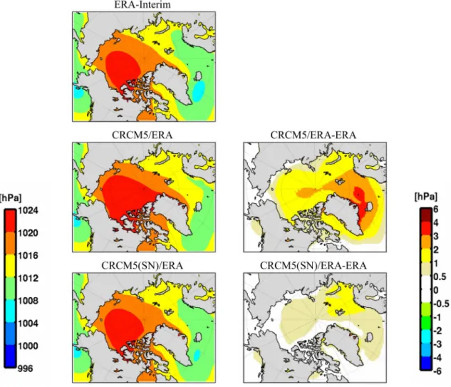
Fig. 3 Left column: Spring mean sea level pressure (hPa) for the 1981–2010 period, from ERA-Interim, CRCM5 without and with large-scale
3 Hindcast climate simulations driven by reanalyses
Hindcast simulations (noted CRCM5/ERA) are used to evaluate structural biases of CRCM5 over the CORDEX Arctic domain, upon assuming that LBC and SSC derived from reanalysis are quasi perfect, therefore the identified biases result from the structure of the model: its formulation, approximations and parameterizations. The CRCM5 simu-lation driven by ERA-Interim using the technique of large-scale spectral nudging will be referred to as CRCM5(SN)/ ERA. The simulations over the time period 1981–2010 will be compared to available observational datasets.
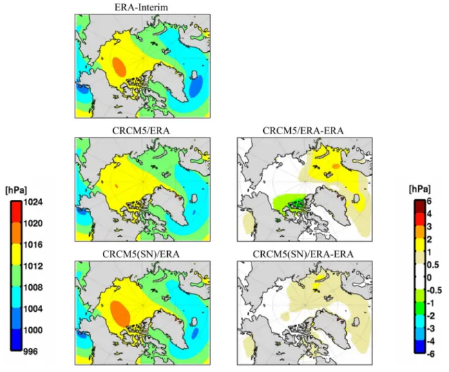
The spring (MAM) and autumn (SON) mean sea level pressure (MSLP) from ERA-Interim reanalysis (ERA), CRCM5 simulation driven by ERA-Interim (CRCM5/ERA), and spectrally-nudged CRCM5 simulation CRCM5(SN)/ ERA are shown in Figs. 3 and 4 respectively, along with the simulation bias (CRCM5 simulation minus ERA-Interim). A mask has been applied over the land area in order to focus the attention away from regions where topography-induced biases
appear due to pressure reduction from the surface height to sea level. The CRCM5 simulation reproduces the overall features of MSLP for all seasons. Spectral nudging is most effective for reducing biases: in spring positive biases are reduced from 4 to 1 hPa over the Greenland Sea (Fig. 3), while in autumn the negative bias of 2 hPa over the Beaufort sea is completely reduced and over the Barents sea while the positive bias of 3 hPa is reduced to 1 hPa (Fig. 4). The bias for winter and summer is around 2–3 hPa (Figs. S1 and S2 respectively in supplementary material). The seasonal-mean time correla-tion between 6-hourly MSLP from ERA and simulated by CRCM5/ERA with and without SN can be found in supple-mentary material (Fig. S3); as expected the time correlations of the CRCM5 simulation using SN technique are notably higher especially over central Arctic Ocean in all seasons.
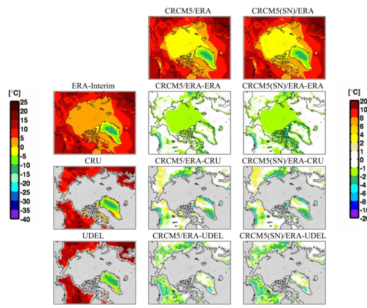
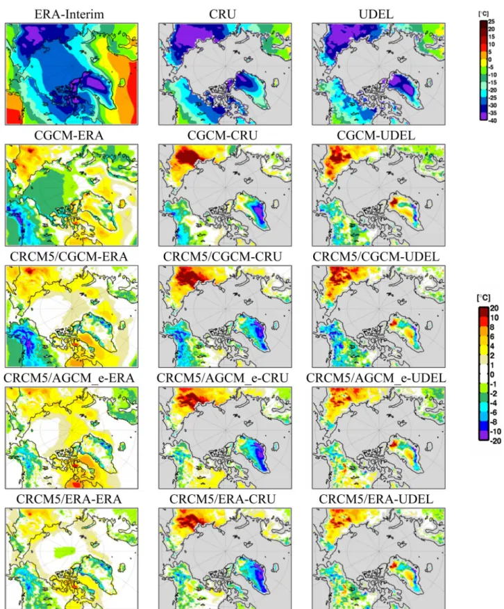
In case of 2-m temperature (T2m), the different observa-tionally-based gridded datasets exhibit substantial differences amongst themselves, and hence the apparent biases of CRCM5 simulation vary considerably depending on the reference data set used. In winter (DJF, Fig. 5), there is an apparent large warm bias over Siberia that reaches 20 °C and a cold bias over
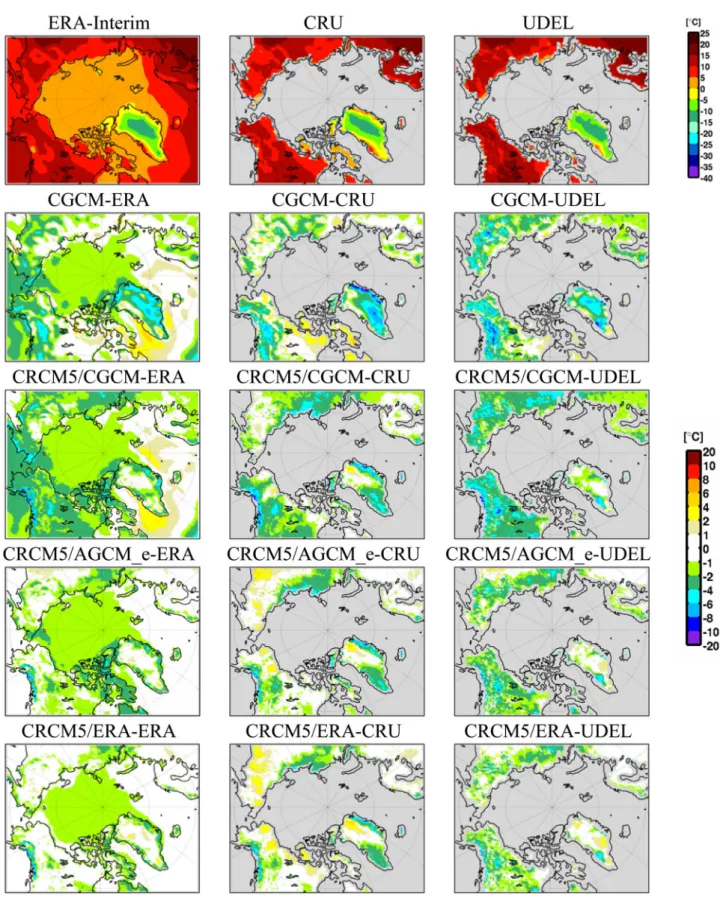
southeastern Greenland of similar magnitude when compared to CRU. Using UDEL as reference, these biases are halved. It is important to keep in mind that in the Arctic area, because of the lack of in situ observations, observational datasets might be biased too. The bias of T2m is smaller during summer (JJA, Fig. 6), the model has a 1 to 2 °C cold bias over the Arctic Ocean when compared to ERA-Interim reanalysis, and variable apparent biases elsewhere depending on the reference dataset used. The magnitude of the bias during MAM and SON is simi-lar to that of JJA (not shown). The effect of simi-large-scale spectral nudging on T2m is negligible as shown in Figs. 5 and 6.
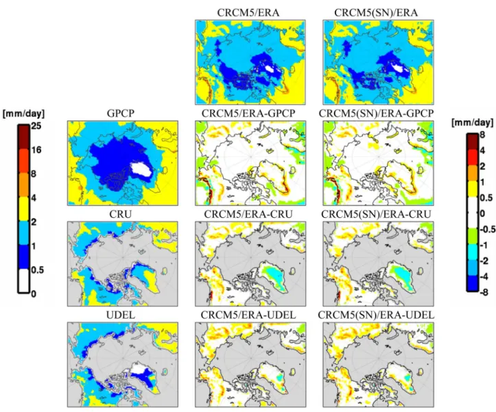
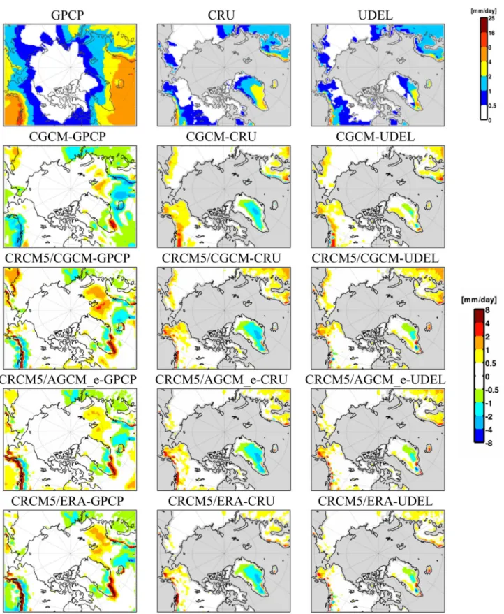
Figures 7 and 8 present CRCM5-simulated precipitation for winter (DJF) and summer (JJA) compared to those from GPCP, CRU and UDEL datasets. The biases are largest in coastal areas with pronounced topography due to different
representation of orographic precipitation, especially during winter (Fig. 7) and autumn (not shown); the apparent bias of CRCM5 simulations is smaller relative to UDEL. Generally the apparent precipitation bias when compared to GPCP is larger in winter than in summer, possibly because of the dif-ficulty for the model to adequately simulate winter clouds and precipitation, or for the satellite-based GPCP to distin-guish clouds from snow cover. The simulated precipitation with and without SN is very similar.
4 Historical climate simulations driven by GCM
In this section, we analyse the results of CRCM5 historical simulations driven by MPI-ESM-MR (CRCM5/CGCM) and Fig. 5 DJF 2-m temperature (˚C) averaged over 1981–2010. In the
first column, observational data from ERA-Interim, CRU and UDEL (second to fourth rows, respectively). In the top row, CRCM5
simu-lations without SN and with SN (second and third columns, respec-tively). The other panels show the differences between the simulation shown in the top row and the reference dataset in the first column
compare it with the results of 3-step dynamical downscal-ing with the empirically corrected SST (CRCM5/AGCM_e). The subscript e is used as a reminder of the empirical correc-tion applied to sea-surface temperature. Because the GCM-driven RCM simulations are affected with inherent bound-ary condition uncertainties in addition to the RCM’s own structural bias, we also compare the bias of the dynamical downscaling simulations to the bias of driving CGCM over the CORDEX Arctic domain.
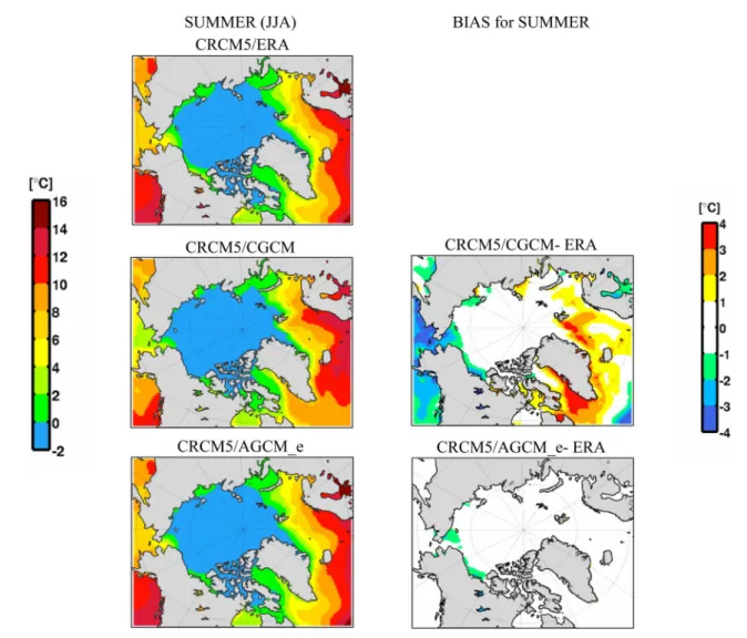
Figure 9 (winter) and Fig. 10 (summer) show the SST fields (left column) and SST biases compared to ERA-Interim (right column), for the CRCM5/ERA, CRCM5/ CGCM and CRCM5/AGCM_e simulations for 1981–2010. Clearly, CRCM5/ERA SST is just the ERA-Interim SST interpolated on the CRCM5 grid, and hence its bias is nil. The CRCM5/CGCM SST was interpolated from the MPI-ESM-MR and reflects the aforementioned biases over open
oceans. Note that where sea ice is present, the SST assumes the freezing temperature of sea water (assumed to be −1.9 °C), and hence the SST bias vanishes when CGCM and ERA-Interim agree on the presence of sea ice. The CRCM/ AGCM_e SST consists of the CGCM SST empirically cor-rected using ERA-Interim, and hence the bias should van-ish in principle. Areas with non-vanvan-ishing CRCM/AGCM_e SST bias reflect where the SST correction could not be applied due to conflicting values of SIC in CGCM and ERA-Interim. The spring bias is very similar to that of winter, but the autumn bias is zero because sea ice extent is usually at its minimum during this season (not shown).
In Fig. 11 transient-eddy standard deviation of the mean sea level pressure is shown for all seasons. This figure dem-onstrates the acceptable ability of CRCM5 to capture daily variability of MSLP. Greater amplitude of the transient eddy near southern tip of Greenland in wintertime indicates the Fig. 6 As Fig. 5, but for JJA
storm track related to SLP difference of Icelandic low and Azores high. The difference between CRCM5 simulations with and without SN as well as CRCM5 simulations driven by CGCM and AGCM_e is relatively modest.
Transient-eddy standard deviation of 2-m temperature (T2m) in supplementary material (Fig. S4) indicates that largest temperature variability over Siberia than over the Arctic Ocean during autumn, probably as a result of the smaller thermal inertia of continent compared to ocean. All CRCM5 simulations standard deviations are smaller than ERA-Interim. Figure S5 shows precipitation transient-eddy which is rather small as expected, except for orographic pre-cipitation in coastlines.
The T2m fields and their biases computed with respect to ERA-Interim, CRU and UDEL are shown in Figs. 12 and
13 for winter and summer, respectively. The comparison of
CGCM and CRCM5/CGCM simulations shows the added value of CRCM5 by a reduction of the T2m bias with respect to ERA over the Arctic Ocean in winter (Fig. 12). The com-parison of CRCM5/CGCM and CRCM5/AGCM_e shows a positive impact of SST correction through a reduction of the T2m bias over North Pacific Ocean and North Atlantic Ocean in all seasons, as well as over the Bering Sea in sum-mer (Fig. 13). Moreover, comparing CRCM5/CGCM and CRCM5/AGCM_e, the SST correction reduces some of the biases over the land and the remaining biases are compa-rable to those seen with CRCM5/ERA. The bias reduction for MAM and SON are similar to those of DJF and JJA, respectively (not shown).
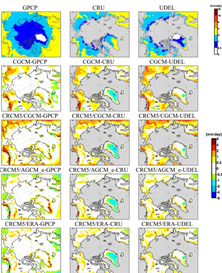
Figures 14 and 15 show the climatological average pre-cipitation bias for 1981–2010 with respect to different ref-erence datasets (GPCP, CRU and UDEL). In JJA (Fig. 15), Fig. 7 DJF precipitation (mm/day) averaged over 1981–2010. In the
first column, observational data from GPCP, CRU and UDEL (sec-ond to fourth rows, respectively). In the top row, CRCM5 simulations
without SN and with SN (second and third columns, respectively). The other panels show the differences between the simulation shown in the top row and the reference dataset in the first column
a large wet bias near the lateral boundaries is noted for the CRCM5/CGCM simulation, which seems to reflect a lateral spin-up problem. The CRCM5/AGCM_e simulation does not suffer from such problem; this constitutes an improve-ment due to the use of the 3-step DD in which the RCM is driven by data simulated by a global model that shares the same physics. Otherwise, the SST correction in the 3-step approach shows little impact for precipitation, in all seasons.
5 Climate change projections
Uncertainty in future climate projections is inevitable; mod-ellers try to present different plausible climate projections. In this study the climate projections using CRCM5 with 2-step DD and 3-step DD (with SSTs bias correction) are compared to the CGCM (MPI-ESM-MR) projections. The representative greenhouse gases concentration pathway used
here for the future projections is RCP8.5, which is one of the greenhouse gases scenario recommended by CORDEX.
Figure 16 shows the CRCM5/AGCM_e sea-ice concen-tration (SIC) for 30 years from 2071 to 2100 in the left col-umn, and the change of SIC between future (2071–2100) and recent past (1981–2010) in the right column. Since SIC is not corrected, the CRCM5/AGCM_e SIC corresponds essentially to that projected by the CGCM, except for very small differences resulting from grid interpolations. The largest SIC decline is projected to occur during autumn, with more than 60% reduction over a vast area of the Arctic Ocean, particularly in East Siberian, Laptev and Kara seas, resulting in a nearly late summer ice-free Arctic Ocean by the end of 21st century. In summer there is a projected 40% SIC reduction over all Arctic Ocean, with a most dramatic reduction near Port of Barrow and Franz Josef Land. Winter and spring exhibit a smaller shrinking sea ice, with the larg-est reduction in Kara and Chukchi seas.
The left column of Fig. 17 shows the CGCM-projected SST climate change between future (2071–2100) and present (1981–2010), displayed after interpolation on the CRCM5 grid (CRCM5/CGCM). Most regions exhibit warming as expected, except a region south of Iceland and Greenland that is projected to become colder. Such cooling is likely related to a slowdown of the Atlantic meridional overturn-ing circulation (AMOC). Several observational studies (e.g., Rahmstorf et al. 2015; Kelly et al. 2016) have documented that a slowdown of the AMOC has already begun to occur in the 20th century, particularly after 1970.
The right column of Fig. 17 shows the corresponding SST climate change in the AGCM_e simulation with empiri-cal SST bias correction, displayed after interpolation on the CRCM5 grid (CRCM5/AGCM_e). In principle, the bias correction is designed in such a way that the resulting SST climate change is unaffected by the correction. In practice, however, the SST correction is not applied whenever there is sea ice present; otherwise the resulting corrected SST would
be incoherent with the SIC field. Figure 17 reveals that there are local small differences between the CRCM5/CGCM (left column) and CRCM5/AGCM_e (right column). For example the warming in CRCM5/AGCM_e is larger over Bering sea in spring and over Beaufort sea in summer.
The T2m projections of CRCM5/CGCM and CRCM5/ AGCM_e are compared to the CGCM projections in Fig. 18. Winter (first column) and then autumn (last column) show the largest climate change with overall similar patterns in all three projections. The maximum warming is projected to occur in winter in the Kara and Beaufort Seas, with values approaching 22 °C in the area of maximum loss of sea ice concentration. Over the Beaufort sea, the CGCM projects a larger warming than CRCM5/AGCM_e and CRCM5/ CGCM. Over land in winter, both CRCM5 projections show less warming over Alaska compared to the CGCM projec-tion, while in summer, they project more warming in the same area (third column). Warming over the Arctic Ocean in summer is a minimum, about 2–4 °C, due to the fact that Fig. 9 DJF SST averaged over 1981–2010, as simulated by CRCM5/ERA (first row), CRCM5/CGCM (second row), CRCM5/AGCM_e (third
in the presence of partial sea-ice coverage, the temperature of water and melting sea-ice remain near the freezing point. Both CRCM5 projections, particularly CRCM5/AGCM_e, anticipate a warmer summer in the end of 21st century than CGCM driving model over land in general. In spring (sec-ond column), CGCM tends to project slightly warmer T2m over lands than CRCM5/CGCM projections. In autumn, a more intense warming projected over central Arctic Ocean by CGCM is notable. There is not much difference in T2m between CRCM5 projections driven by CGCM or AGCM_e during autumn and spring (Fig. 18).
Figure 19 displays the projected precipitation changes over the future period 2071–2100 compared to the refer-ence period 1981–2010, for DJF (left column) and JJA (right column). In Fig. 20 the relative precipitation change is also shown. Both CRCM5 simulations for winter project a precipitation increase up to 6 mm/day in North Pacific and Scandinavian wet coastal areas, compared to values of less than 2 mm/day for CGCM. All models project some
reduction in the North Atlantic or south of Greenland, although the patterns are not consistent and the percent change is less than 25%. This decrease is likely related to the projected cooling point in the North Atlantic. Some studies such as Koenigk et al. (2015) have suggested that precipita-tion and temperature changes in the future are somehow lin-early related; the projected precipitation increase over Kara sea and Bering sea, where the largest warming is projected, tends to confirm that hypothesis. It also is in accordance with the suggested link between local sea ice loss, tropospheric warming and finally precipitation increase by Rinke and Dethloff (2008). There is a noteworthy difference between the projected precipitation changes by CRMC5/CGCM and CRCM5/AGCM_e in summer, with CRCM5/AGCM_e sug-gesting a widespread reduction (0.5 mm/day) for continental areas surrounding the Arctic Ocean.
Projected MSLP changes are shown for each season in supplementary material (Fig. S6). By the end of this century, a general decrease in MSLP is projected over the Arctic Fig. 10 As Fig. 9, but for JJA
Ocean for all seasons, with the largest decrease reaching 8 hPa being projected in autumn and winter for the region close to the Bering straight. A weak increase of MSLP is projected for the North Sea, largest in spring, and in some models in winter or summer. This implies an overall increase in westerly flow south of Greenland, and an increase of south-westerly flow over the North sea that corresponds to warmer air flowing from mid-latitudes, coherent with
warming and sea-ice loss over the Arctic.We can try to put these projections for the end of the century in perspective with studies of recent warming over the Arctic. Some studies noted that reduced autumn ice extent leads to an atmospheric winter circulation that resembles the negative phase of the North Atlantic Oscillation (NAO), with cold winter tem-perature anomalies in Eastern Europe, e.g. Koenigk et al. (2016). More recent studies however note that the observed Fig. 11 Transient-eddy standard deviation of mean sea level pressure
(MSLP) for each season averaged over 1981–2010. First row is from ERA-Interim, and following rows correspond to various CRCM5
simulations: CRCM5/ERA without SN and with SN are shown in second and third rows, CRCM5/CGCM (fourth row), and CRCM5/ AGCM_e (fifth row)
Fig. 12 DJF 2-m temperature averaged over 1981–2010, from the
references in the first row as ERA-Interim (first column), CRU ond column) and UDEL (third column). The biases of CGCM
(sec-ond row), CRCM5/CGCM (third row), CRCM5/AGCM_e (fourth row) and CRCM5/ERA in (fifth row) with every reference are shown in the corresponding column
Fig. 14 In the top row, DJF precipitation (mm/day) averaged over
1981–2010, from three references: GPCP (first column), CRU ond column) and UDEL (third column). The biases of CGCM
(sec-ond row), CRCM5/CGCM (third row), CRCM5/AGCM_e (fourth row) and CRCM5/ERA (fifth row) with every reference are shown in the corresponding column
trends are not robust when tested over longer time periods and that they seem to be at least partly caused by natural variations (Koenigk and Brodeau 2017). So there does not
seem to be conclusive links between the projected climate and the recent variations of temperature and circulation over the Arctic and mid-latitudes.
6 Summary and conclusions
In this study, the skill of CRCM5 hindcast simulations driven by ERA-Interim reanalysis, the effectiveness of the large-scale spectral nudging (SN), and future climate-change projections using 2- and 3-step dynamical downs-caling over the CORDEX Arctic domain were investigated. The performance of the new version of Canadian Regional Climate Model (CRCM5) has been assessed by comparing a CRCM5 hindcast simulation driven by a reanalysis with
different observational references such as gridded in situ observations, and satellite-based datasets, as well as ERA-Interim reanalysis, considering the 30-year historical period from 1981 to 2010. The CRCM5 shows an adequate skill to capture overall features of mean sea level pressure (MSLP) for all seasons. The largest bias was found in spring, with a bias of 4 hPa, which was reduced to 1 hPa using SN. The CRCM5 simulations driven by ERA-Interim with and with-out SN are similar for surface air temperature (T2m) and precipitation. The apparent bias in T2m largely depends on Fig. 16 Seasonal mean sea-ice concentration (SIC) for the future
period 2071–2100, projected by CRCM5/AGCM_e (first column), for winter, spring, summer and autumn (in first to fourth rows,
respec-tively). The second column shows the corresponding SIC changes (2071–2100) – (1981–2010)
the reference dataset that is used. The bias with respect to the CRU dataset is twice that compared to UDEL. The T2m bias is larger in winter.
The overall amount of Arctic precipitation is very low. Its maximum amount in the domain is found in coastal areas subject to orographic precipitation, reaching 16 mm/day
in autumn. Minimum precipitation occurs over the Arctic Ocean, with values less than 1 mm/day in spring and winter. In summer, the regions with the highest level of precipita-tion are located in European part of the Arctic and North Pacific Ocean, with around 8 mm/day. The precipitation bias of CRCM5 simulations when compared to the GPCP Fig. 17 Seasonal mean SST changes (2071–2100) to (1981–2010) projected by CRCM5/CGCM (first column) and by CRCM5/AGCM_e
dataset is more pronounced in coastal areas. In general, this bias becomes considerably larger than the apparent bias with respect to UDEL. The lack of reliable precipitation obser-vational datasets for the pan-Arctic region makes it nearly impossible to evaluate objectively the skill of CRCM5 to reproduce precipitation pattern. Surface stations are scarce and satellite remote sensing procedures could be biased as well, due to the difficulty in distinguishing cloud from snow/ ice cover.
We also analysed the impact of using empirically cor-rected sea surface temperature (SST). The significantly improved results of CRCM5 historical simulations over CORDEX-Africa domain using this strategy (Hernández-Díaz et al. 2016) motivated us to perform such method over Arctic domain. The outputs of CGCM (MPI-ESM-MR in our case) are always biased, resulting in part from their coarse resolution. In this approach, we subtracted the SST bias calculated over an historical period from the mean cli-matological simulations over the same period. In the next step, we used this corrected SST as sea-surface boundary condition for an atmosphere-only global model (AGCM) simulation. Finally, the output of this intermediate step is used as atmospheric lateral boundary conditions to drive
CRCM5. The importance of the intermediate AGCM simu-lation is to make a compatible combination of lower and lateral boundary conditions (keep the physical coherence between the atmosphere and the correct SST). Note however that unlike in Hernández-Díaz et al. (2016), no correction has been applied to sea-ice concentration (SIC). When-ever the corrected SST was found to be incoherent with the CGCM-simulated SIC, it was adjusted to be coherent with SIC.
Positive impact of SST correction are seen through a reduction of the T2m bias over North Pacific Ocean and North Atlantic Ocean in all seasons, as well as over the Ber-ing Sea in summer. This method showed a little impact on precipitation simulation over Arctic region. In contrast to Africa, the capability of improving the simulation appears limited since the presence of sea ice over a large fraction of the domain restricted the regions where SST correction could be applied. Note, however, that although the improve-ment in simulated precipitation is relatively small, it is a positive consequence of the 3-step DD, due to the use of the same physics in the AGCM and RCM.
Future projections of CGCM were compared with those performed with CRCM5 driven by CGCM (CRCM5/ Fig. 18 Projected changes (2071–2100) to (1981–2010) for 2-m
temperature by CGCM (first row), CRCM5/CGCM (second row), CRCM5/AGCM_e (third row). The first column is specified for
win-ter and the second, third and last are specified for spring, summer and autumn respectively
CGCM) and driven by the AGCM using bias-corrected SST (CRCM5/AGCM_e). For conciseness, the analysis of the future projections was restricted to the period from 2071 to 2100, under the scenario RCP8.5 following one of the CORDEX recommendations. The CGCM-projected SIC shows very large reduction, 40–60% in summer and 60–100% in autumn, hence a nearly ice-free Arctic Ocean is projected by the end of 21st century. The maximum projected sea surface temperature is 16 °C in North Pacific
Ocean and some other small zones during summer (not shown). Projections show 8 °C warming of sea surface temperature during JJA, over Kara and Chukchi Seas and a slight cooling of −1 °C in North Atlantic Ocean during cold seasons.
For T2m, the largest projected warming is 22 °C in two regions near Kara and Chukchi Seas in winter. The CRCM5/AGCM_e and CRCM5/CGCM project less warm-ing than the CGCM durwarm-ing winter and more warmwarm-ing Fig. 19 Projected changes (2071–2100) to (1981–2010) for precipitation by CGCM (first row), CRCM5/CGCM (second row), CRCM5/
during summer over Alaska by 2100. Both CRCM5 simu-lations project less warming over the Arctic Ocean for fall compared to the CGCM simulation.
An overall 0.5–2 mm/day increase in precipitation is projected, while in very narrow coastal bands increase is up to 6 mm/day. For summer, CRCM/AGCM_e pro-jects widespread decreasing precipitation unlike CGCM and CRCM5/CGCM, but the decrease is modest, about 0.5 mm/day.
Acknowledgements This research was funded in part by the
follow-ing grants: the project “Marine Environmental Observation, Predic-tion and Response” (MEOPAR; http://meopar.ca) of the Networks of Centres of Excellence (NCE; http://www.nce-rce.gc.ca) of Canada, the Discovery Accelerator Supplements Program ( http://www.nserc-crsng.gc.ca/Professors-Professeurs/Grants-Subs/DGAS-SGSA_eng. asp) of the Natural Sciences and Engineering Research Council of Canada (NSERC; http://www.nserc-crsng.gc.ca), the Canadian Net-work for Regional Climate and Weather Processes (CNRCWP; http:// www.cnrcwp.uqam.ca) funded by the NSERC Climate Change and Atmospheric Research (CCAR; http://www.nserc-crsng.gc.ca/
Professors-Professeurs/Grants-Subs/CCAR-RCCA_eng.asp) program, and the Ouranos Consortium on Regional Climatology and Adapta-tion to Climate Change (http://www.ouranos.ca). Computations were made on the supercomputer Guillimin of Calcul Québec - Compute Canada (http://www.calculquebec.ca) whose operation is funded by the Canada Foundation for Innovation (CFI), NanoQuébec, RMGA and the Fonds de recherche du Québec - Nature et technologies (FRQ-NT). The authors thank Mr Georges Huard and Mrs Nadjet Labassi for maintaining an efficient and user-friendly local computing facility. This study would not have been possible without the access to valuable data such as ERA-Interim, CRU, GPCP and TRMM, as well as outputs from the CMIP5 database, in this case the MPI-ESM-LR model output.
Open Access This article is distributed under the terms of the
Creative Commons Attribution 4.0 International License ( http://crea-tivecommons.org/licenses/by/4.0/), which permits unrestricted use, distribution, and reproduction in any medium, provided you give appro-priate credit to the original author(s) and the source, provide a link to the Creative Commons license, and indicate if changes were made.
References
ACIA (2004) Impacts of a warming Arctic. Arctic climate impact assessment. http://www.acia.uaf.edu. http://www.cambridge. org. Cambridge University Press.
Adler RF, Huffman GJ, Chang A, Ferraro R, Xie P, Janowiak J, Rudolf B, Schneider U, Curtis S, Bolvin D, Gruber A, Susskind J, Arkin P (2003) The version 2 global precipitation climatology project (GPCP) monthly precipitation analysis (1979–present). J Hydrometeor 4:1147–1167
Alexandru A, Sushama L (2015) Current climate and climate change over India as simulated by the Canadian regional climate model. Clim Dyn 45:1059–1084. doi:10.1007/s00382-014-2350-y Arakawa A, Lamb VR (1977) Computational design of the basic
dynamical process of the UCLA general circulation model. Methods Comput Phys 17:173–265
Bélair S, Mailhot J, Girard C, Vaillancourt PA (2005) Boundary layer and shallow cumulus clouds in a medium-range forecast of a large-scale weather system. Mon Weather Rev 133:1938–1960. doi:10.1175/MWR2958.1
Bélair S, Roch M, Leduc A-M, Vaillancourt PA, Laroche S, Mail-hot J (2009) Medium-range quantitative precipitation forecasts from Canada’s new 33-km deterministic global operational system. Weather Forecast 24:690–708. doi:10.1175/2008 WAF2222175.1
Benoit R, Côté J, Mailhot J (1989) Inclusion of a TKE boundary layer parameterization in the Canadian regional finite-element model. Mon Weather Rev 117:1726–1750
Berg P, Döscher R, Koenigk T (2013) Impacts of using spectral nudg-ing on regional climate model RCA4 simulations of the Arctic. Geosci Model Dev 6:849–859. doi:10.5194/gmd-6-849-2013 Biner S, Caya D, Laprise R, Spacek L (2000) Nesting of RCMs by
imposing large scales. Research activities in atmospheric and oce-anic modelling, WMO/TD 987. Report 30:7.3–7.4
Bruyère CL, Done JM, Holland GJ, Fredrick S (2014) Bias cor-rections of global models for regional climate simulations of high-impact weather. Clim Dyn 43:1847–1856. doi:10.1007/ s00382-013-2011-6
Chapman WL, Walsh JE (2007) Simulations of Arctic temperature and pressure by global coupled models. J Clim 20:609–632. doi:10.1175/JCLI4026.1
Christensen JH, Christensen OB (2007) A summary of the PRU-DENCE model projections of changes in European climate by
the end of this century. Clim Change 81:7–30. doi:10.1007/ s10584-006-9210-7
Côté J, Gravel S, Méthot A, Patoine A, Roch M, Staniforth A (1998) The operational CMC-MRB global environmental multiscale (GEM) model. Part I: design considerations and formulation. Mon Weather Rev 126:1373–1395
Curry JA, Lynch AH (2002) Comparing Arctic Regional climate model. EOS 83:87. doi:10.1029/2002EO000051
Davies HC (1976) A lateral boundary formulation for multi-level pre-diction models. Q J R Meteorol Soc 102:405–418
Dee DP, Uppala SM, Simmons AJ, Berrisford P, Poli P, Kobayashi S, Andrae U, Balmaseda MA, Balsamo G, Bauer P (2011) The ERA-Interim reanalysis: configuration and performance of the data assimilation system. Q J R Meteorol Soc 137:553–597. doi:10.1002/qj.828
Delage Y (1997) Parameterising sub-grid scale vertical transport in atmospheric models under statically stable conditions. Bound Layer Meteorol 82:23–48
Delage Y, Girard C (1992) Stability functions correct at the free con-vection limit and consistent for both the surface and Ekman layers. Bound Layer Meteorol 58:19–31
Déqué M, Alias A, Dubois C, Somot S (2014) Some sources of bias in the Eurocordex historical runs. Third International Lund regional-scale climate modelling workshop. Lund. http://www. baltex-research.eu/RCM2014/index.html. Accessed 22 Sept 2017 Førland EJ, Benestad R, Flatøy F, Hanssen-Bauer I, Haugen JE, Isak-sen K, Sorteberg A, Ådlandsvik B (2009) Climate development in North Norway and the Svalbard region during 1900–2100. RAPPORTSERIE NR. 128, APRIL 2009, NORSK POLARIN-STITUTT, POLARMILJØSENTERET, 9296 TROMSØ. http:// www.npolar.no. Accessed 22 Sept 2017
Glisan JM, Gutowski WJ Jr, Cassano JJ, Higgins ME (2013) Effects of spectral nudging in WRF on Arctic temperature and pre-cipitation simulations. J Clim 26:3985–3999. doi:10.1175/ JCLI-D-12-00318.1
Harris I, Jones PD, Osborn TJ, Lister DH (2014) Updated high-reso-lution grids of monthly climatic observations—the CRU TS3.10 dataset. Int J Climatol 34:623–642. doi:10.1002/joc.3711 Hernández-Díaz L, Laprise R, Sushama L, Martynov A, Winger K,
Dugas B (2013) Climate simulation over the CORDEX-Africa domain using the fifth-generation Canadian regional climate model (CRCM5). Clim Dyn 40:1415–1433. doi:10.1007/ s00382-012-1387-z
Hernández-Díaz L, Laprise R, Nikiéma O, Winger K (2016) 3-Step dynamical downscaling with empirical correction of sea-surface conditions: application to a CORDEX Africa simulation. Clim Dyn 48(7):2215–2233. doi:10.1007/s00382-016-3201-9 IPCC (2013) Climate change 2013: the physical science basis.
Con-tribution of working group I to the fifth assessment report of the intergovernmental panel on climate change. In: Stocker TF, Qin D, Plattner GK, Tignor M, Allen SK, Boschung J, Nauels A, Xia Y, Bex V, Midgley PM (eds) Cambridge University Press, Cam-bridge, p 1535
Kain S, Fritsch JM (1990) A one-dimensional entraining/detraining plume model and its application in convective parameterization. J Atmos Sci 47:2784–2802
Katzfey JJ, McGregor JL, Nguyen K, Thatcher M (2009) Dynami-cal downsDynami-caling techniques: impacts on regional climate change signals. In: 18th World IMACS/MODSIM Congress, Cairns, pp 2377–2383
Katzfey JJ, Chattopadhyay M, McGregor JL, Nguyen K, Thatcher M (2011) The added value of dynamical downscaling. In: 19th international congress on modelling and simulation, Perth, pp 2747–2753
Kelly KA, Drushka K, Thompson L, Le Bars D, McDonagh EL (2016) Impact of slowdown of Atlantic overturning circulation
on heat and freshwater transports. Geophys Res Lett 43:7625– 7631. doi:10.1002/2016GL069789
Keup-Thiel E, Göttel H, Jacob D (2006) Climate simulations for the Barents sea region. Boreal Env Res 11(5):329–339
Koenigk T, Brodeau L (2017) Arctic climate and its interaction with lower latitudes under different levels of anthropogenic warm-ing in a global coupled climate model. Clim Dyn 49:471–492. doi:10.1007/s00382-016-3354-6
Koenigk T, Berg P, Doscher R (2015) Arctic climate change in an ensemble of regional CORDEX simulations. Polar Res. doi:10.3402/polar.v34.24603 (ISSN 1751–8369)
Koenigk T, Caian M, Nikulin G, Schimanke S (2016) Regional Arc-tic sea ice variations as predictor for winter climate conditions. Clim Dyn 46:317–337. doi:10.1007/s00382-015-2586-1 Kuo HL (1965) On formation and intensification of tropical cyclones
through latent heat release by cumulus convection. J Atmos Sci 22:40–63
Laprise R (1992) The Euler equation of motion with hydrostatic pres-sure as independent coordinate. Mon Weather Rev 120:197–207 Laprise R, Hernández-Díaz L, Tete K, Sushama L, Šeparović L, Mar-tynov A, Winger K, Valin M (2013) Climate projections over CORDEX Africa domain using the fifth-generation Canadian regional climate model (CRCM5).Clim Dyn 41:3219–3246. doi:10.1007/s00382-012-1651-2
Li J, Barker HW (2005) A radiation algorithm with correlated-k distribution. Part I: local thermal equilibrium. J Atmos Sci 62:286–309
Lucas-Picher P, Somot S, Déqué M, Decharme B, Alias A (2013) Evaluation of the regional climate model ALADIN to simulate the climate over North America in the CORDEX framework. Clim Dyn 41:1117–1137. doi:10.1007/s00382-012-1613-8
Martynov A, Sushama L, Laprise R (2010) Simulation of temperate freezing lakes by one-dimensional lake models: performance assessment for interactive coupling with regional climate mod-els. Boreal Environ Res 15:143–164 (ISSN 1797–2469 online;
ISSN 1239–6095 print)
Martynov A, Sushama L, Laprise R, Winger K, Dugas B (2012) Inter-active lakes in the Canadian regional climate model, version 5: the role of lakes in the regional climate of North America. Tellus A 64:16226–16245. doi:10.3402/tellusa.v64i0.16226
Martynov A, Laprise R, Sushama L, Winger K, Šeparović L, Dugas B (2013) Reanalysis-driven climate simulation over CORDEX North America domain using the Canadian regional climate model, version 5: model performance evaluation. Clim Dyn 41:2973–3005. doi:10.1007/s00382-013-1778-9
Masson V, Champeaux J-L, Chauvin F, Meriguet C, Lacaze R (2003) A global database of land surface parameters at 1-km resolution in meteorological and climate models. J Clim 16:1261–1282 McFarlane NA (1987) The effect of orographically excited gravity wave
drag on the circulation of the lower stratosphere and troposphere. J Atmos Sci 44:1175–1800
Overland J, Hanna E, Hanssen-Bauer I, Kim SJ, Walsh JE, Wang M, Bhatt US (2014) Surface air temperature. Update for 2014, Arctic report card
Paquin JP, Sushama L (2014) On the Arctic near-surface permafrost and climate sensitivities to soil and snow model formulations in climate models. Clim Dyn 44(1–2):255–277
Rahmstorf S, Box JE, Feulner G, Mann ME, Robinson A, Ruther-ford S, Schaffernicht EJ (2015) Exceptional twentieth-century slowdown in Atlantic Ocean overturning circulation. Nat Clim Change 5(5):475–480 (ISSN 1758-678X)
Ramsayer K (2014) Antarctic sea ice reaches new record maximum. http://climate.nasa.gov/news/2169/antarctic-sea-ice-reaches-new-record-maximum/. Accessed 22 Sept 2017
Richter I (2015) Climate model biases in the eastern tropical oceans: causes, impacts and ways forward. WIREs Clim Change 6(3):345–358. doi:10.1002/wcc.338
Rinke A, Dethloff K (2000) On the sensitivity of a regional Arc-tic climate model to initial and boundary conditions. Clim Res 14:101–113
Rinke A, Dethloff K (2008) Simulated circum-Arctic climate changes by the end of the 21st century. Glob Planet Change 62:173–186 Rinke A, Marbaix P, Dethloff K (2004) Internal variability in Arctic regional climate simulations: case study for the SHEBA year. Clim Res 27:197–209
Rinke A, Dethloff K, Cassano JJ, Christensen JH, Curry JA, Du P, Girard E, Haugen JE, Jacob D, Jones CG, Koltzow M, Laprise A, Lynch AH, Pfeifer S, Serreze MC, Shaw MJ, Tjernstorm M, Wyser K, Zagar M (2006) Evaluation of an ensemble of Arctic regional climate models: spatiotemporal fields dur-ing the SHEBA year. Clim Dyn 26:459–472. doi:10.1007/ s00382-005-0095-3
Rinke A, Matthes H, Christensen JH, Kuhry P, Romanovsky VE, Dethloff K (2012) Arctic RCM simulations of temperature and precipitation derived indices relevant to future frozen ground conditions. Glob Planet Change 80–81:136–148
Šeparović L, Alexandru A, Laprise R, Martynov A, Sushama L, Winger K, Tete K (2013) Present climate and climate change over North America as simulated by the fifth-generation Canadian regional climate model. Clim Dyn 41:3167–3201. doi:10.1007/s00382-013-1737-5
Steiner N, Azetsu-Scott K, Galbraith P, Hamilton J, Hedges K, Hu X, Janjua MY, Lambert N, Larouche P, Lavoie D, Loder J, Mel-ling H, Merzouk A, Myers P, Perrie W, Peterson I, Pettipas R, Scarratt M, Sou T, Starr M, Tallmann RF, van der Baaren A (2013) Climate change assessment in the Arctic basin part 1: trends and projections—a contribution to the Aquatic Climate Change Adaptation Services Program. Can Tech Rep Fish Aquat Sci 3042:xv + 163
Stendel M, Christensen JH, Petersen D (2008) Arctic Climate and Climate Change with a Focus on Greenland. Adv Ecol Res 40:13–43. doi: 10.1016/s0065-2504(07)00002-5
Sundqvist H, Berge E, Kristjansson JE (1989) Condensation and cloud parameterization studies with a mesoscale numerical weather prediction model. Mon Weather Rev 117:1641–1657 van der Linden P, Mitchell JFB (eds) (2009) ENSEMBLES: climate
change and its impacts: summary of research and results from the ENSEMBLES project. Met Office Hadley Centre, Exeter, p 160 Verseghy LD (2000) The Canadian land surface scheme (CLASS):
its history and future. Atmos Ocean 38:1–13
Verseghy LD (2008) The Canadian land surface scheme: technical documentation—version 3.4. Climate Research Division, Sci-ence and Technology Branch, Environment Canada
von Storch H, Langenberg H, Feser F (2000) A spectral nudging tech-nique for dynamical downscaling purposes. Mon Weather Rev 128:3664–3673. doi:10.1175/1520-0493(2000)128<3664:ASN TFD>2.0.CO;2
Willmott CJ, Matsuura K (1995) Smart interpolation of annually averaged air temperature in the United States. J Appl Meteorol 34:2577–2586
Yeh K-S, Côté J, Gravel S, Méthot A, Patoine A, Roch M, Stani-forth A (2002) The CMC–MRB global environmental multi-scale (GEM) model. Part III: nonhydrostatic formulation. Mon Weather Rev 130:339–356
Yu M, Wang G (2014) Impacts of bias correction of lateral boundary conditions on regional climate projections in West Africa. Clim Dyn 42:2521–2538. doi:10.1007/s00382-013-1853-2
Zadra A, Roch M, Laroche S, Charron M (2003) The subgrid-scale orographic blocking parametrization of the GEM model. Atmos Ocean 41:155–170
Zadra A, McTaggart-Cowan R, Roch M (2012) Recent changes to the orographic blocking. In: Seminar presentation, RPN, Dor-val, Canada, 30 March 2012. http://collaboration.cmc.ec.gc.ca/ science/rpn/SEM/dossiers/2012/seminaires/2012-03-30/Semi-nar_2012-03-30_Ayrton-Zadra.pdf. Accessed 19 July 2012 Zhang J, Krieger J, Bhatt U, Lu C, Zhang X (2016) Alaskan
regional climate changes in dynamically downscaled CMIP5
simulations. In: Uzochukwu G, Schimmel K, Kabadi V, Chang SY, Pinder T, Ibrahim S (eds) Proceedings of the 2013 national conference on advances in environmental science and technology. Springer, Cham. doi:10.1007/978-3-319-19923-8_5