Science Arts & Métiers (SAM)
is an open access repository that collects the work of Arts et Métiers Institute of Technology researchers and makes it freely available over the web where possible.
This is an author-deposited version published in: https://sam.ensam.eu Handle ID: .http://hdl.handle.net/10985/6522
To cite this version :
Amine AMMAR, Elias CUETO, David GONZALEZ, Francisco CHINESTA - Towards a high-resolution numerical strategy based on separated representations - 2008
Any correspondence concerning this service should be sent to the repository Administrator : [email protected]
Towards a high-resolution numerical strategy based on separated
representations
D. Gonz´alez
1, A. Ammar
2, E. Cueto
1, F. Chinesta
31Group of Structural Mechanics and Material Modelling.
Arag´on Institute of Engineering Research (I3A). University of Zaragoza. Mar´ıa de Luna, 5.
Campus Rio Ebro. E-50018 Zaragoza, Spain. e-mail: {gonzal,ecueto}@unizar.es;
2Laboratoire de Rh´eologie, UMR 5520, Universit´e J. Fourier
1301 Rue de la piscine. Domaine universitaire,
38041 Grenoble Cedex, France. e-mail: [email protected];
3Laboratoire de M´ecanique des Syst´emes et des Proc´ed´es.
UMR 8106 CNRS-ENSAM-ESEM
151 Boulevard de l’Hˆopital, F-75013 Paris, France e-mail: [email protected] ABSTRACT: Many models in Science and Engineering are defined in spaces (the so-called conformation spaces) of high dimensionality. In kinetic theory, for instance, the micro scale of a fluid evolves in a space whose number of dimensions is much higher than the usual physical space (two or three). Models defined in such a framework suffer from the curse of dimensionality, since the complexity of the problem growths ex-ponentially with the number of dimensions. This curse of dimensionality makes this class of problems nearly intractable if we perform a standard discretization, say, with finite element methods, for instance. Problems defined in two or three-dimensional spaces, but densely discretized along each spatial dimension are also hardly tractable by finite element methods. In this paper we present some recent results concerning a method based on the method of separation of variables, originally developed in [1]. We focus on an efficient imposition of essential non-homogeneous boundary conditions and the treatment of problems with a very high number of degrees of freedom.
KEYWORDS: Curse of dimensionality, separation of variables, high-dimensional problems, kinetic theory 1 INTRODUCTION
In problems that involve high dimensional spaces, standard discretization techniques, like the finite el-ement method, fail due to an excessive computation time required to perform accurate numerical simula-tions.
The main aim of this paper is to present a new nu-merical strategy able to circumvent some of the dif-ficulties due to the multidimensional character of ki-netic theory models, among other fields of science. The results will be presented to illustrate its capability for treating highly dimensional spaces by considering different multidimensional Poisson’s problems, and an efficient imposition of essential non-homogeneous boundary conditions.
2 THE METHOD
For simplicity, we start by considering the Poisson problem defined in a space of dimension N with ho-mogeneous boundary conditions,
−∆T = f (x1, x2, . . . , xN) in Ω = (−L, L)N. (1) The problem solution can be written in the form
T (x1, x2, . . . , xN) ≈ Q X j=1 αj N Y k=1 Fkj(xk), (2) where Fkj is the jth basis function, with unit norm, and only depends on the kth coordinate. Note that the solution of numerous problems can be accurately ap-proximated using a finite number Q of approximation functions.
The numerical scheme proposed consist of an it-eration procedure that solves at each itit-eration n the following three steps.
Step 1 A projection step of the solution in a discrete basis, where the coefficients αj are computed. Step 2 Convergence checking.
Step 3 Enrichment of the approximation basis step. From the coefficients αj just computed the ap-proximation basis can be enriched by adding the new functionQNk=1Fk(n+1)(xk)
For details of this scheme see [1].
3 IMPOSITION OF NON-HOMOGENEOUS ES-SENTIAL BOUNDARY CONDITIONS
Consider, for simplicity and without loss of general-ity, the Poisson problem described before, see Eq. (1) subjected to the boundary conditions:
T = TD 6= 0 on Γ = ∂Ω. (3) Let us assume that we are able to find a function ψ, continuous in Ω, such that −∆ψ ∈ L2(Ω) verifying
Eq. (3). Then, the solution of the problem given by Eqs. (1)-(3) can be obtained straightforwardly by
T = ψ + z, (4)
where we thus face a problem in the z variable
−∆z = f + ∆ψ in Ω (5)
z = 0 on Γ = ∂Ω, (6)
solvable by the method of separation of variables be-fore presented.
Following this procedure, the weak form of the problem will be: Find z ∈ H1(Ω) such that for every
z∗ ∈ H1 0(Ω) Z Ω ∇z∇z∗dΩ = Z Ω z∗f dΩ − Z Ω ∇ψ∇z∗dΩ (7) holds.
Several choices for the function ψ exist. In this work we employ R-functions [4], which constitute an efficient means of constructing ψ functions.
The obtained function ψ, which is generally not product or sum separable, is separated approximately by employing the Singular Value Decomposition (SVD) technique. To this end, we employ singular values up to a given precision, which is normally set to 10−5.
4 NUMERICAL EXAMPLES
In this section we describe some simple numerical ex-periments that show the potential of the method.
4.1 Example: 2D problem
Let us consider now the problem
∆T = 0 in [−1, 1]2, (8)
subjected to the boundary conditions
T = x2+ y2on ∂Ω,
that in this case do not verify the partial differential equation (8).
In this case, using the before mentioned theory of
R-functions, we obtain the following function
verify-ing essential boundary conditions:
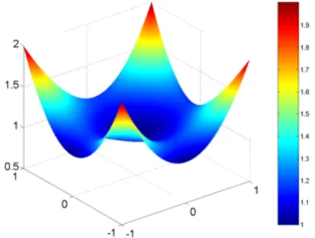
ψ = −2 + x
4+ y4
−2 + x2+ y2 (9)
which is represented in Fig. 1. This function is again not sum or product separable, according to [3]. Ap-plying SVD, we arrive to the one-dimensional func-tions depicted in Fig. 2, that approximate the function
ψ to the chosen level of precision, 10−5 in this case.
Figure 1: Function ψ for the second problem, Eq. (8).
−1 −0.5 0 0.5 1 −0.4 −0.2 0 0.2 0.4 0.6 0.8 1 1.2 1.4 x Fx −1 −0.5 0 0.5 1 −0.4 −0.2 0 0.2 0.4 0.6 0.8 1 1.2 1.4 y Fy
Figure 2: Singular Value Decomposition of ψ up to the
The method before described was applied in meshes composed by 15, 20, 30, 50, 80 and 130 nodes along each spatial direction. The solution was com-pared to one approximate solution obtained by stan-dard Finite Elements in a mesh composed by 40000 nodes, thus taken as exact. The order of convergence is remarkably high, and has been found to be of the or-der of 4 (i.e., superconvergent) for all the cases tested.
dof along each spatial direction
lo g || e rr o r| |L2 20 40 60 80 100 120 -5.5 -5 -4.5 -4 -3.5 1 3.95
Figure 3: Solution convergence obtained by the proposed technique.
4.2 Extension of the proposed technique to higher-dimensional problems
The problem with the straightforward extension of the proposed technique to higher dimensional problems lies in obtaining the appropriate counterpart of the SVD decomposition in high dimensions.
To this end, we have employed the PARAFAC (Parallel Factors) decomposition, also known as CANDECOMP or Canonical Decomposition, pro-vided by the MATLAB tensor toolbox [2]. This tech-nique provides a diagonal tensor Σ, suitable for the purpose of this work. The r most relevant entries of this tensor are employed in the decomposition, in order to accomplish with a user-predefined tolerance in the representation of the function ψ. In general, we seek for decompositions of our function ψ, whose nodal values are stored in an order n (n = 3 in the example here considered, for simplicity of graphical representation) tensor A, in the form:
A = Σ ×1U ×2V ×3W ×4. . . (10)
where Σ is a diagonal tensor and U , V , W , ... are the components or factors of the decomposition. Columns of the factors are orthonormal in standard, two-dimensional SVD, but this is not possible, in gen-eral, in tensors of order three or higher. The products
involved in the previous decomposition are defined as follows: B = C ×1U (11) is such that (B)ljk = m X i=1 CijkUli (12)
To analyze the behavior of the technique, we have extended the previous problem to three-dimensional settings:
∆T = 0 in [−1, 1]3, (13)
subjected to the boundary conditions
T = x2+ y2+ z2on ∂Ω.
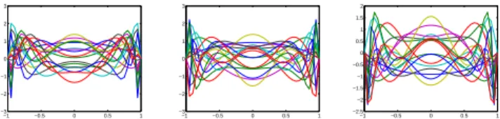
The higher-order SVD decomposition of the func-tion ψ up to the tolerance 10−6provides the functions depicted in Fig. 4. Only four functions along each spatial direction were necessary.
−1 −0.5 0 0.5 1 0.5 1 1.5 2 2.5 3 3.5 4 4.5 5 −1 −0.5 0 0.5 1 1 1.5 2 2.5 3 3.5 4 4.5 5 5.5 −1 −0.5 0 0.5 1 −4 −3 −2 −1 0 1 2 3 4 5
Figure 4: Functions obtained along x (a), y (b) and z (c) spatial directions for the boundary conditions of the problem stated in
Eq. (13).
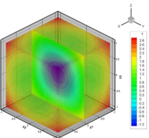
With these functions thus calculated, we let the method run to obtain the solution to the problem as depicted along each direction in Fig. 5. The global, three-dimensional, solution to the problem is depicted in Fig. 6. In this case, 18 functions were necessary along each spatial direction to obtain the before men-tioned accuracy. The figure depicts the intersection of the solution with the plane x = 0.
−1 −0.5 0 0.5 1 −3 −2 −1 0 1 2 3 −1 −0.5 0 0.5 1 −3 −2 −1 0 1 2 3 −1 −0.5 0 0.5 1 −2.5 −2 −1.5 −1 −0.5 0 0.5 1 1.5 2
Figure 5: Functions obtained along x, y and z spatial directions for the problem stated in Eq. (13).
Figure 6: Solution obtained by the proposed technique for the problem with non-homogeneous boundary conditions in three
dimensions. Mesh of 40 elements along each direction.
4.3 A problem with 109 degrees of freedom
In order to show the behavior of the proposed method we have analyzed the problem
∆T = 2(1 − y4)(1 − z6) + 12(1 − x2)y2(1 − z6)+
+ 30(1 − x2)(1 − y4)z4in [−1, 1]3, (14)
(the same analyzed in [1]), subjected to the boundary conditions
T = 0 on ∂Ω,
that has been discretized in a regular lattice of 10003
elements, thus giving 10013 degrees of freedom. This
value is on the limit of current capabilities of nowa-days computers, and is analyzed here only for the purpose of showing the performance of the method. The analytical solution to this problem is given by the function T = (1 − x2)(1 − y4)(1 − z6).
The functions obtained by the method in each spa-tial direction are depicted in Fig. 7. As can be noticed, the method obtains a very accurate solution in only one iteration, as was the case in [1], employing fewer degrees of freedom. −1 −0.5 0 0.5 1 0 0.2 0.4 0.6 0.8 1 −1 −0.5 0 0.5 1 0 0.1 0.2 0.3 0.4 0.5 0.6 0.7 0.8 0.9 −1 −0.5 0 0.5 1 0 0.1 0.2 0.3 0.4 0.5 0.6 0.7 0.8
Figure 7: Functions obtained along x, y and z spatial directions for the problem stated in Eq. (14).
The solution obtained is represented in Fig. 8(top), where a downsampling has been applied to the results by employing a coarser mesh. For obvi-ous reasons, it is difficult to depict the results on a mesh of 109 nodes. The error obtained is depicted in
Fig. 8(bottom), where a slice on an arbitrary section of the domain has been performed for clarity.
X -1 -0.5 0 0.5 1 Y -1 -0.5 0 0.5 1 Z -1 -0.5 0 0.5 1 X Y Z T 0.95 0.9 0.85 0.8 0.75 0.7 0.65 0.6 0.55 0.5 0.45 0.4 0.35 0.3 0.25 0.2 0.15 0.1 0.05
Figure 8: Solution of the problem stated in Eq. (7) and a slice on the error map.
In this example we do not pursue accuracy, but testing the possibility of employing a huge number of degrees of freedom. What is noticeable about this solution, easily reachable with traditional Finite Ele-ments, is that, despite the extremely high number of degrees of freedom involved, the Matlab code ran in around 1 hour on a PC with four processors (only one was employed, no parallel calculation was allowed) with 1.96 Gb of RAM memory each, running under Linux. This time comprised data file writing, genera-tion of figures, etc.
REFERENCES
[1] A. Ammar, B. Mokdad, F. Chinesta, and R. Keunings. A new family of solvers for some classes of multidimensional partial differential equations encountered in kinetic theory modeling of complex fluids. J. Non-Newtonian Fluid Mech., 139:153–176, 2006.
[2] Brett W. Bader and Tamara G. Kolda. Efficient MATLAB computations with sparse and factored tensors. SIAM
Jour-nal on Scientific Computing, July 2007. Accepted.
[3] M. Messiter and Y. Shamash. Product and sum separa-ble functions. IEEE Transactions on Automatic Control, (7):694–697, 1985.
[4] V. L. Rvachev and T. I. Sheiko. R-functions in boundary value problems in mechanics. Applied Mechanics reviews, 48:151–188, 1995.