The Water Isotopic Version of the Land-Surface Model ORCHIDEE: Implementation, Evaluation, Sensitivity to Hydrological Parameters

HAL Id: hal-02473896

https://hal.archives-ouvertes.fr/hal-02473896

Submitted on 27 May 2020

HAL is a multi-disciplinary open access

archive for the deposit and dissemination of

sci-entific research documents, whether they are

pub-lished or not. The documents may come from

teaching and research institutions in France or

abroad, or from public or private research centers.

L’archive ouverte pluridisciplinaire HAL, est

destinée au dépôt et à la diffusion de documents

scientifiques de niveau recherche, publiés ou non,

émanant des établissements d’enseignement et de

recherche français ou étrangers, des laboratoires

publics ou privés.

Hydrological Parameters

Camille Risi, Jerome Ogee, Sandrine Bony, Thierry Bariac, Naama Raz

Yaseef, Lisa Wingate, Jeffrey Welker, Alexander Knohl, Cathy Kurz Besson,

Monique Leclerc, et al.

To cite this version:

Camille Risi, Jerome Ogee, Sandrine Bony, Thierry Bariac, Naama Raz Yaseef, et al.. The Water

Isotopic Version of the Land-Surface Model ORCHIDEE: Implementation, Evaluation, Sensitivity to

Hydrological Parameters. Hydrology: Current Research, HILARIS Publisher, 2016, 07 (04), pp.1-24.

�10.4172/2157-7587.1000258�. �hal-02473896�

Open Access Research Article

*Corresponding author: Camille Risi, LMD/IPSL, CNRS, UPMC, Paris, France, Tel:

+33144276272; E-mail: crlmd@lmd.jussieu.fr

Received August 30, 2016; Accepted September 24, 2016; Published October

01, 2016

Citation: Risi C, Ogée J, Bony S, Bariac T, Raz-Yaseef N, et al. (2016) The

Water Isotopic Version of the Land-Surface Model ORCHIDEE: Implementation, Evaluation, Sensitivity to Hydrological Parameters. Hydrol Current Res 7: 258. doi: 10.4172/2157-7587.1000258

Copyright: © 2016 Risi C, et al. This is an open-access article distributed under

the terms of the Creative Commons Attribution License, which permits unrestricted use, distribution, and reproduction in any medium, provided the original author and source are credited.

The Water Isotopic Version of the Land-Surface Model ORCHIDEE:

Implementation, Evaluation, Sensitivity to Hydrological Parameters

Camille Risi1_{*, Jerome Ogée}2_{, Sandrine Bony}1_{, Thierry Bariac}3_{, Naama Raz-Yaseef}4,5_{, Lisa Wingate}2_{, Jeffrey Welker}6_{, Alexander Knohl}7_,

Cathy Kurz-Besson8_{, Monique Leclerc}9_{, Gengsheng Zhang}9_{, Nina Buchmann}10_{, Jiri Santrucek}11,12_{, Marie Hronkova}11,12_{, Teresa David}13_,

Philippe Peylin14 _{and Francesca Guglielmo}14

1_{LMD/IPSL, CNRS, UPMC, Paris, France} 2_{INRA Ephyse, Villenave d’Ornon, France}

3_{UMR 7618 Bioemco, CNRS-UPMC-AgroParisTech-ENS Ulm-INRA-IRD-PXII Campus AgroParisTech, Bâtiment EGER, Thiverval-Grignon, 78850 France} 4_{Earth Sciences Division, Lawrence Berkeley National Laboratory, Berkeley, USA}

5_{Department of Environmental Sciences and Energy Research, Weizmann Institute of Science, PO Box 26, Rehovot 76100, Israel} 6_{Biology Department and Environment and Natural Resources Institute, University of Alaska, Anchorage, AK 99510, USA} 7_{Bioclimatology, Faculty of Forest Sciences and Forest Ecology, Georg-August University of Göttingen, 37077 Göttingen, Germany} 8_{Instituto Dom Luiz, Centro de Geofísica IDL-FCUL, Lisboa, Portugal}

9_{University of Georgia, Griffin, GA 30223, USA}

10_{Institute of Agricultural Sciences, ETH Zurich, Zurich, Switzerland} 11_{Biology Centre ASCR, Branisovska 31, Ceske Budejovice, Czech Republic}

12_{University of South Bohemia, Faculty of Science, Branisovska 31, Ceske Budejovice, Czech Republic} 13_{Instituto Nacional de Investigação Agrária e Veterinária, Quinta do Marquês, Portugal}

14_{LSCE/IPSL, CNRS, UVSQ, Orme des Merisiers, Gif-sur-Yvette, France}

Abstract

Land-Surface Models (LSMs) exhibit large spread and uncertainties in the way they partition precipitation into surface runoff, drainage, transpiration and bare soil evaporation. To explore to what extent water isotope measurements could help evaluate the simulation of the soil water budget in LSMs, water stable isotopes have been implemented in the ORCHIDEE (ORganizing Carbon and Hydrology In Dynamic EcosystEms: the land-surface model) LSM. This article presents this implementation and the evaluation of simulations both in a stand-alone mode and coupled with an atmospheric general circulation model. ORCHIDEE simulates reasonably well the isotopic composition of soil, stem and leaf water compared to local observations at ten measurement sites. When coupled to LMDZ (Laboratoire de Météorologie Dynamique-Zoom: the atmospheric model), it simulates well the isotopic composition of precipitation and river water compared to global observations. Sensitivity tests to LSM (Land-Surface Model) parameters are performed to identify processes whose representation by LSMs could be better evaluated using water isotopic measurements. We find that measured vertical variations in soil water isotopes could help evaluate the representation of infiltration pathways by multi-layer soil models. Measured water isotopes in rivers could help calibrate the partitioning of total runoff into surface runoff and drainage and the residence time scales in underground reservoirs. Finally, co-located isotope measurements in precipitation, vapor and soil water could help estimate the partitioning of infiltrating precipitation into bare soil evaporation.

Keywords: Water isotopes; Land-surface model; Global models; Soil water budget; Rain infiltration; Runoff; Evapo-transpiration partitioning

Introduction

Land-surface models (LSMs) used in climate models exhibit a large spread in the way they partition radiative energy into sensible and latent heat [1,2] precipitation into evapo-transpiration and runoff [3-5], evapo-transpiration into transpiration and bare soil evaporation [6,7], and runoff into surface runoff and drainage [8-10]. This results in an large spread in the predicted response of surface temperature [11] and hydrological cycle [12,13] to climate change [11] or land use change [14,15]. Therefore, evaluating the accuracy of the partitioning of precipitation into surface runoff, drainage, transpiration and bare soil evaporation (hereafter called the soil water budget) in LSMs is crucial to improve our ability to predict future hydrological and climatic changes.

The evaluation of LSMs is hampered by the difficulty to measure over large areas the different terms of the soil water budget, notably the evapo-transpiration terms and the soil moisture storage [16,17]. Single point measurements of evapo-transpiration fluxes [18] and soil moisture [19] are routinely performed within international networks, but those measurements remain difficult to upscale to a climate model grid box due to the strong horizontal heterogeneity of the land surface [20,21]. Spatially-integrated data such as river runoff observations are very valuable to evaluate soil water budgets at the regional scale [22,23],

but are insufficient to constrain the different terms of the water budget. Additional observations are therefore needed.

In this context, water isotope measurements have been suggested to help constrain the soil water budget [24,25], its variations with climate or land use change [26], and its representation by large-scale models [27,28]. For example, water stable isotope measurements in the different water pools of the soil-vegetation-atmosphere continuum have been used to quantify the relative contributions of transpiration and bare soil evaporation to evapo-transpiration [29-32], to infer plant source water depth [33], to assess the mass balance of lakes [34-36] or to investigate pathways from precipitation to river discharge [37-40]. These isotope-based techniques generally require high frequency isotope measurements and are best suitable for intensive field campaigns at the local scale. At larger spatial and temporal scales, some

Page 2 of 24 attempts have been made to use regional gradients in precipitation

water isotopes for partitioning evapo-transpiration into bare soil-evaporation and transpiration [41-43].

To explore to what extent water isotope measurements could be used to evaluate and improve land surface parameterizations, water isotopes were implemented in the LSM ORCHIDEE (ORganizing Carbon and Hydrology In Dynamic EcosystEms [44,45]. This isotopic version of ORCHIDEE has already been used to explore how tree-ring cellulose records past climate variations [46] and to investigate the continental recycling and its isotopic signature in Western Africa [47] and at the global scale [48].

The first goal of this article is to evaluate the isotopic version of the ORCHIDEE model against recently-made-available new datasets combining water isotopes in precipitation, vapor, soil water and rivers. The second goal is to evaluate the isotopic version of the ORCHIDEE model when coupled to the atmospheric General Circulation Model (GCM) LMDZ (Laboratoire de Météorologie Dynamique Zoom [49]). The third goal is to perform sensitivity tests to LSM parameters to identify processes whose representation by LSMs could be better evaluated using water isotopic measurements.

After introducing notations and models in section 4, we present ORCHIDEE simulations in a stand-alone mode at measurement sites and global ORCHIDEE-LMDZ coupled simulations.

Notation and Models

Notations

H O H O) in the different water

pools are expressed in‰ relative to a standard: = sample 1 1000

SMOW R R

δ  − ⋅

  , where

R_sample and R_SMOW are the isotopic ratios of the sample and of the Vienna

Standard Mean Ocean Water (V-SMOW) respectively [50,51]. To

first order, variations in δD are similar to those in δ18_{O but are 8 times}

larger. Deviation from this behavior can be associated with kinetic

fractionation and is quantified by deuterium excess (d=δD-8.δ18_O

[50,52]). Hereafter, we note δ18_O

p, δ18Ov, δ18Os, δ18Ostem and δ18Oriver the

δ18_{O of the precipitation, atmospheric vapor, soil, stem, river water}

respectively. The same subscripts apply for d.

The LMDZ model

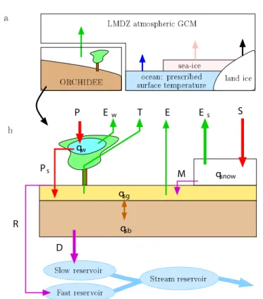
LMDZ is the atmospheric GCM (General Circulation Model) of the IPSL (Institut Pierre Simon Laplace) climate model [53,54]. We use the LMDZ-version 4 model [49] which was used in the International Panel on CLimate Change’s Fourth Assessment Report simulations [55,56]. The resolution is 2.5 ° in latitude, 3.75 ° in longitude and 19 vertical levels. Each grid cell is divided into four sub-surfaces: ocean, land ice, sea ice and land (treated by ORCHIDEE) (Figure 1a). All parameterizations, including ORCHIDEE, are called every 30 min. The implementation of water stable isotopes is similar to that in other GCMs [57,58] and has been described in [59,60]. LMDZ captures reasonably well the spatial and seasonal variations of the isotopic composition in precipitation [60] and water vapor [61].

The ORCHIDEE (ORganizing Carbon and Hydrology In

Dynamic EcosystEms: the land-surface model) model

The ORCHIDEE model is the LSM component of the IPSL climate model. It merges three separate modules: (1) SECHIBA (Schématisation des EChanges Hydriques a l’Interface entre la Biosphère et l’Atmosphère [44,62]) that simulates land-atmosphere water and energy exchanges, (2) STOMATE (Saclay-Toulouse-Orsay

Model for the Analysis of Terrestrial Ecosystems [45]) that simulates vegetation phenology and biochemical transfers ; and (3) LPJ (Lund-Postdam-Jena [63]) that simulates the vegetation dynamics. Water stable isotopes were implemented in SECHIBA, and we use prescribed land cover maps so that the two other modules could be de-activated.

Each grid box is divided into up to 13 land cover types: bare soil, tropical broad-leaved ever-green, tropical broad-leaved rain-green, temperate needle-leaf ever-green, temperate broad-leaved ever-green, temperate broad-leaved summer-green, boreal needle-leaf ever-green, boreal broad-leaved summer-green, boreal needle-leaf summer-green, C3 grass, C4 grass, C3 agriculture and C4 agriculture. Water and energy budgets are computed for each land cover type.

Figure 1b illustrates how ORCHIDEE (ORganizing Carbon and Hydrology In Dynamic EcosystEms: the land-surface model) represents the surface water budget. Rainfall is partitioned into interception by the canopy and through-fall rain. Through-fall rain, snow melt, dew and frost fill the soil. The soil is represented by two water reservoirs: a superficial and a bottom one [64,65]. Taken together, the two reservoirs have a water holding capacity of 300 mm and a depth of 2 m.

qw D qsg qsb P Ew T Es S M E qsnow R Ps

Figure 1: a) The four sub-surfaces in the LMDZ GCM: land, ocean, sea ice

and land ice. Their relative fraction in each grid box is prescribed. The sea surface temperature of the ocean is prescribed, and interactively calculated for sea-ice and land-ice. Over land, the land-Surface model (LSM) ORCHIDEE calculates interactively the surface temperature and outgoing water fluxes. b) Water fluxes and pools represented in the ORCHIDEE LSM. Water pools

are the soil water in the superficial (qsg) and bottom (qsb) layers, the water

intercepted by the canopy (qw) and the snow pack (qsnow). Fluxes onto the

land surface are the total rain (P) and snow (S), and possibly dew or frost.

As some rain is intercepted by the canopy, only throughfall rain (Ps) arrives at

the soil surface. Evaporation fluxes are the evaporation of intercepted water

(Ew), transpiration by the vegetation (T), bare soil evaporation (E) and snow

sublimation (Es). Snow melt may be transferred from the snow pack to the soil

(M). Water from rainfall, melt (and possibly dew) exceeding the soil capacity is converted to surface runoff (R) and drainage (D). The routing model then transfers surface runoff and drainage to streams.

Page 3 of 24 Soil water undergoes transpiration by vegetation, bare soil evaporation

or runoff. Transpiration and evaporation rates depend on soil moisture to represent water stress in dry conditions. Runoff occurs when the soil water content exceeds the soil holding capacity and is partitioned into 95% drainage and 5% surface runoff [66]. Snowfall fills a single-layer snow reservoir, where snow undergoes sublimation or melt. By comparison, when not coupled to ORCHIDEE, the simple bucket-like LSM in LMDZ makes no distinction neither between bare soil evaporation and transpiration nor between surface runoff and drainage [67].

Surface runoff and drainage are routed to the coastlines by a water routing model [68]. Surface runoff is stored in a fast ground water reservoir which feeds the stream reservoir with residence time of 3 days. Drainage is stored in a slow ground water reservoir which feeds the stream reservoir with residence time of 25 days. The water in the stream reservoir is routed to the coastlines with a residence time of 0.24 days.

Implementation of water stable isotopes in ORCHIDEE

We represent isotopic processes in a similar fashion as other isotope-enabled LSMs [69-73]. Some details of the isotopic implementation are described in Risi [74]. In absence of fractionation, water stable isotopes

( 16 2 H O_, 18 2 H O, HDO, 17 2

H O_{) are passively transferred between the different}

water reservoirs. We assume that surface runoff has the isotopic composition of the rainfall and snow melt that reach the soil surface. Drainage has the isotopic composition of soil water [24]. We calculate the isotopic composition of bare soil evaporation or of evaporation of water intercepted by the canopy using the Craig and Gordon equation [75] (Equation 3). We neglect isotopic fractionation during snow sublimation (Equation 2). We consider isotopic fractionation at the leaf surface (Equation 5) but we assume that transpiration has the isotopic composition of the soil water extracted by the roots (Equation 2).

In the control coupled simulation, we assume that the isotopic composition of soil water is homogeneous vertically and equals the weighted average of the two soil layers. However, transpiration, bare soil evaporation, surface runoff and drainage draw water from different soil water reservoirs whose isotopic composition is distinct [76-78]. Therefore, we also implemented a representation of the vertical profile of the soil water isotopic composition.

Stand-alone ORCHIDEE Simulations at MIBA

(Moisture in Biosphere and Atmosphere: Network for

Water Isotopes in Soil, Stem and Leaf Water) and

Carbo-Europe Measurement Sites

First, we performed simulations using ORCHIDEE as a

stand-alone model at ten sites. Using isotopic measurements in soil, stem and leaf water, simulations are evaluated at each site at the monthly scale. Sensitivity tests to evapo-transpiration partitioning and soil infiltration processes are performed.

Measurements used for evaluation

To first order the composition of all land surface water pools is driven by that in the precipitation [79]. Therefore, a rigorous evaluation of an isotope-enabled LSM requires to evaluate the difference between the composition in each water pool and that in the precipitation. Besides, to better isolate isotopic biases, we need a realistic atmospheric forcing. We tried to select sites where (1) isotope were measured in different water pools of the soil-plant-atmosphere continuum, during at least a full seasonal cycle and (2) meteorological variables were monitored at a frequency high enough (30 minutes) to ensure robust forcing for our model and (3) water vapor and precipitation were monitored to provide isotopic forcing for the LSM. Only two sites satisfy these conditions: Le Bray and Yatir. Relaxing some of these conditions, we got a more a representative set of ten sites representing diverse climate conditions (Table 1 and Figure 2).

Description of the ten sites: The ten sites belong to two kinds of observational networks: MIBA (Moisture Isotopes in the Biosphere and Atmosphere [80-82] or Carbo-Europe [83,84].

Le Bray site, in South-Eastern France, joined the MIBA and GNIP (Global Network for Isotopes in Precipitation) network in 2007. It is an even-aged Maritime pine forest with C3 grass understory that has been the subject of many eco-physiological studies since 1994, notably as part of the Carbo-Europe flux network [85]. In 2007 and 2008, samples in precipitation, soil surface, needles, twigs and atmospheric vapor

were collected every month and analyzed for δ18_{O following the MIBA}

protocol [82,86]. This site was also the subject of intensive campaigns where soil water isotope profiles were collected between 1993 and 1997, and in 2007 [87].

The Yatir site, in Israel, is a semi-arid Aleppo pine forest. It is an afforestation growing on the edge of the desert, with mean-annual precipitation of 280 mm [88,89]. It has also been the subject of many eco-physiological studies as part of the Carbo-Europe flux network [89] and joined the MIBA network in 2004. It. In 2004-2005, samples of soil water at different depth, stems and needles were collected following the MIBA protocol. The water vapor isotopic composition has been monitored daily at the nearby Rehovot site (31.9 ° N, 34.65 ° E, [90]) and is used to construct the water vapor isotopic composition forcing. We must keep in mind however that although only 66 km from Yatir, Rehovot is much closer to the sea and is more humid than Yatir. The precipitation isotopic composition has been monitored monthly at

Site name Country Location Network Years Reference

Le Bray France 44.70° N, 0.77° W MIBA, Carbo- Euroe 2007-2008 [87]

Yatir Israel 31.33° N, 35.0° E MIBA, Carbo-Euroe 2004-2005 [89,104]

Morgan-Monroe United States 39.32° N, 86.42° W MIBA-US 2005-2006 [167,172]

Donaldson Forest United States 29.8° N, 82.163° W MIBA-US 2005-2006 [91,169]

Anchorage United States 61.2° N, 149.82° W MIBA-US 2005-2006

-Mitra Portugal 38.5° N, 8.00° W Carbo-Euroe 2001-2002 [171]

Bily Kriz Czech Republic 49.5° N, 18.53° E MIBA, Carbo-Euroe 2005 [92]

Brloh Czech Republic 49.80° N, 14.66° E MIBA 2004-2010 [93]

Hainich Germany 50.97° N, 13.57° E Carbo-Euroe 2001-2002 [170]

Tharandt Germany 51.08° N, 10.47° E Carbo-Euroe 2001-2002

-Table 1: Information on the 10 sites used in this study: geographical location, network the sites are part of, years during which the istopic measurements were made and

Page 4 of 24

the nearby GNIP station Beit Dagan (32 ° N, 34.82 ° E) and is used to construct the precipitation isotopic composition forcing.

The Morgan-Monroe State Forest, Donaldson Forest and Anchorage sites are part of the MIBA-US (MIBA-United States) network and are located in Indiana, in Florida and in Alaska respectively (Table 1). Sampling took place in 2005 and 2006 according to the MIBA protocols. The Donaldson Forest site, which jointed the MIBA-US network in 2005, is located at the AmeriFlux Donaldson site near Gainesville, Florida, USA. The site is flat with an elevation of about 50 m. It was covered by a forest of managed slash pine plantation, with an uneven understory composed mainly of saw palmetto, wax myrtle and Carolina jasmine [91]. The leaf area index was measured during a campaign in 2003 and estimated at 2.85. We use this value in our simulations.

The Mitra, Bily Kriz, Brloh, Hainich and Tharandt sites are part of the Carbo-Europe project. Hainich and Tharandt are located in Germany. The experimental site of Herdade da Mitra (230 m altitude, nearby Évora in southern Portugal) is characterized by a Mediterranean mesothermic humid climate with hot and dry summers. It is a managed agroforestry system characterized by an open evergreen woodland sparsely covered with Quercus suber L. and Q. ilex rotundifolia trees (30 trees/ha), with an understorey mainly composed of Cistus shrubs, and winter-spring C3 annuals. The isotopic samplings of leaves, twigs, soil, precipitation and groundwater were performed on a seasonal to monthly basis. All samples where extracted and analyzed at the Paul Scherrer Institute (Switzerland).

Bily Kriz and Brloh are both located on the Czech Republic. Bily Kriz is an experimental site in Moravian–Silesian Beskydy Mountains (936 m a.s.l.) with detailed records of environmental conditions [92]. It is dominated by Norway spruce forest. It joined the MIBA project in the season 2005. Brloh is a South Bohemian site in the Protected Landscape Area Blanskýles (630 m a.s.l.). It is dominated by deciduous beech forest and was used as MIBA sampling site from 2004 to 2010 [93].

Isotopic measurements: Samples of soil water, stems and leaves were collected at the monthly scale. The MIBA and MIBA-US protocols recommend sampling the first 5-10 cm excluding litter and the

Carbo-Europe protocol recommends sampling the first 5 cm [84], but in practice the soil water sampling depth varies from site to site. At some sites, soil water was sampled down to 1 m. For evaluating the seasonal

evolution of soil water δ18_{O, we focus on soil samples collected in the}

first 15 cm only. Observed full soil water δ18_{O profiles were used only}

at Le Bray and Yatir for evaluating the shape of simulated soil water

δ18_{O profiles.}

Carbo-Europe samples were extracted and analyzed at the Department of Environmental Sciences and Energy Research, Weizmann Institute of Science, Israel. MIBA-US samples were extracted and analyzed at the Center for Stable Isotope Biogeochemistry

of the University of California, Berkeley. Analytical errors for δ18_{O in}

soil, stem and leaf water vary from 0.1‰ to 0.2‰ depending on the sites and involved stable isotope laboratory (Table 2).

Meteorological, turbulent fluxes and soil moisture measurements: At most of the sites, meteorological parameters (radiation, air temperature and humidity, soil temperature and moisture) are continuously measured and are used to construct the meteorological forcing for ORCHIDEE.

Fluxes of latent and sensible energy are measured using the eddy co-variance technique and are used for evaluating the hydrological simulation. Gaps are filled using ERA-Interim reanalyses [94]. Soil moisture observations are available at most sites.

Simulation set-up

To evaluate in detail the isotope composition of different water pools, stand-alone ORCHIDEE simulations on the ten MIBA and Carbo-Europe sites were performed. We prescribe the vegetation type and properties and the bare soil fraction based on local knowledge at each site (Table 3).

ORCHIDEE offline simulations require as forcing several meteorological variables: near-surface temperature, humidity and winds, surface pressure, precipitation, downward longwave and shortwave radiation fluxes. At Le Bray and Yatir, we use local meteorological measurements available at hourly time scale. At other

0.1

0.5

1

2

3

4

annual−mean precipitation (mm/d)

MMSF

DOFO

BFOA

Tharandt

Hainich

Brloh

Mitra

Le Bray

Bily Kriz

Yatir

70N

50N

30N

10N

160W

100W

40W

20E

60E

Figure 2: Location of the ten stations used in this study for single-point model-data comparison. The background represents the annual-mean precipitation

from GPCP (Global Precipitation Climatology Project) to illustrate the diversity of climate regimes covered by the ten stations. Each station is described in more detail in Table 1.

Page 5 of 24

are not available on the other sites. Therefore, we create isotopic forcing using isotopic measurements in the precipitation performed on nearby GNIP or USNIP stations. To interpolate between the nearby stations, we take into account spatial gradients and altitude effects by exploiting outputs from an LMDZ simulation.

Model-data comparison methods

Simulated isotopic composition in soil, stem and leaf water: The soil profile option is activated in all our stand-alone ORCHIDEE simulations. We compare the soil water samples collected in the first 15 cm of the soil (in the first 5-10 cm at many sites) to the soil water composition simulated in the uppermost layer.

The observed composition of stem water is compared to the simulated composition of the transpiration flux.

When comparing observed and simulated composition of leaf water, the Peclet effect, which mixes stomatal water with xylem water (Equation 8), is deactivated. Neglecting the Peclet effect may lead to

overestimate of δ18_O

leaf values.

sites, we use local meteorological measurements when available and combine them with ERA-Interim reanalyses at 6-hourly time scale for missing variables. At other sites, no nearby meteorological measurements are available and only ERA-Interim reanalyses [94] are used (Table 3).

At each site, we run the model three times over the first year of isotopic measurement (e.g., 2007 at Le Bray). These three years are discarded as spin-up. Then we run the model over the full period of isotopic measurements (e.g., 2007-2008 at Le Bray). We checked

that at all sites, the seasonal distribution of δ18_{O, which is the slowest}

variable to spin-up, is identical between the last year of spin-up and the following year.

We force ORCHIDEE with monthly isotopic composition of precipitation and near-surface water vapor. Since we evaluate the results at the monthly time scale, we assume that monthly isotopic forcing is sufficient. At Le Bray and Yatir, monthly observations of isotopic composition of precipitation and near-surface water vapor are available to construct the forcing. Unfortunately, these observations

Site name Biome Dominant Species _{temperature (°C)}Annual-mean Annual-mean precipitation

(mm/year) Elevation (m)

Le Bray Temperate coniferous forest Maritime pine 12 1022 60

Yatir semi-arid forest Aleppo pine 15.3 270 650

Morgan-Monroe Temperate deciduous forest Liriodendron tulipifera 12.4 1094 275

Donaldson Forest Tropical pine plantation Pinus palustris 21.7 1330 50

Anchorage Boreal coniferous forest Picea glauca 2.3 408 35

Mitra Mediteranean forest Sparse holm oak trees with _{patches of cork trees} 13.9 480 230

Bily Kriz Temperate coniferous forest Pine forest 3.4 1024 936

Brloh Temperate deciduous forest Beech forest 7.6 832 630

Hainich Temperate deciduous forest Fagus Sylvatica 8 800 440

Tharandt Temperate deciduous forest Pine forest 8.1 1000 380

Table 2: Vegetation and climtological information on the 10 sites used in this study: biome, dominant species, annual-mean temperature and precipitation, elevation.

Site name Prescribe vegetation in ORCHIDEE Meteoro-logical _{forcing precipitation and vapor}Isotopic forcing for _{stations used to calculate isotopic forcing}local, GNIP, USNIP or Carbo-Europe

Le Bray 70% temperate needleleaf evergreen (LAI=0.4), 30% _{C3 grass (LAI=0.4)} obs obs_iso Le Bray local data for both precipitation and _{water vapor}

Yatir 100% temperate needleleaf evergreen (LAI=4) obs obs_iso Rehovot for water vapor and Beit Dagan _{GNIP station for precipitation}

Morgan-Monroe 100% temperate broad-leaved summergreen _(LAI=4.5) obs_ERA NIP_LMDZ USNIP_IN22, USNIP_KY03

Donaldson Forest 100% temperate needleleaf evergreen (LAI=2.85) obs_ERA NIP_LMDZ USNIP_FL14, USNIP_FL99

Anchorage 40% boreal needle-leaved evergreen (LAI=4), 60% _{boreal broad-leaved summergreen (LAI=4.5)} ERA NIP_LMDZ Bethel, USNIP_SOGR_10, USNIP_CA45

Mitra 50% temperate broad-leaved evergreen (LAI=2), 50% _{C3 grass (LAI=0.4)} obs_ERA NIP_LMDZ Beja, Faro, Penhas, Mitra, Portoallegre

Bily Kriz 100% temperate needleleaf evergreen (LAI=7.5) obs_ERA NIP_LMDZ Vienna, Podersdorf, Apetlon, Liptovsky, _Krakow

Brloh 100% temperate broad-leaved summergreen _(LAI=4.5) ERA NIP_LMDZ Leipzig, Hohhohensaas, Regensburg, Vienna, _{Petzenkirchen}

Hainich 80% temperate broad-leaved summergreen _{(LAI=4.5), 20% C3 grass (LAI=0.4)} obs_ERA NIP_LMDZ _{BadSalzuflen, Wuerzburg, Wasserkuppe}Leipzig, Hohhohensaas, Braunschweig,

Tharandt 80% temperate needleleaf evergreen (LAI=4), 20% _{C3 grass (LAI=0.4)} obs_ERA NIP_LMDZ Leipzig, Berlin, Hohhohensaas, Regensburg

Table 3: Information on the offline simulations performed on the 10 sites listed in Table 1: meteorological forcing (6 hourly observations of temperature, humidity, winds,

precipitation and radiative fluxes), isotopic forcing (monthly isotopic composition of the precipitation and near-surface water vapor), and prescribed vegetation type and LAI (leaf area index) properties. We give proportions (in %) of the total vegetated area, excluding bare soil. For example, if a given vegetation type covers 100% of the vegetated area and the bare soil fraction is 30%, then the vegetation type covers only 70% of the total area. Three kinds of meteorological forcing are possible: meteorological observations only (obs), meteorological observations filled with ERA-Interim for missing variables (obs_ERA) or ERA-Interim (ERA). Two kinds of isotopic forcing are possible: isotopic composition of precipitation and water vapor observed on the site (obs_iso), or interpolation between GNIP, USNIP or Carbo-Europe stations using the LMDZ atmospheric general circulation model. In the former case, the datasets used for prescribing the water vapor and precipitation isotopic composition forcing are mentionned. In the latter case, GNIP, USNIP or Carbo-Europe stations used to construct the interpolated precipitation isotopic composition forcing are listed.

Page 6 of 24 Impact of the temporal sampling: Over the ten sites, samples

were collected during specific days and hours. This temporal sampling may induce artifacts when comparing observations to monthly-mean simulated ORCHIDEE values. For soil and stem water, the effect of temporal sampling can be neglected because simulated soil and stem water composition vary at a very low frequency. For leaf water however, there are large diurnal variations [95]. For example, if leaf

water is sampled every day at noon when δ18_O

leaf is maximum, then

observed δ18_O

leaf will be more enriched than monthly-mean δ18Oleaf. The

exact sampling time is available for Le Bray site only, where we will estimate the effect of temporal sampling.

Spatial heterogeneities: We are aware of the scale mismatch between punctual in-situ measurements and an LSM designed for large scales (a typical GCM grid box is more than 100 km wide). However, for soil moisture it has been shown that local measurements represent a combination of small scale (10-100 m) variability [20,21] and a large-scale (100-1000 km) signal [96] that a large-scale model should capture [97]. The sampling protocol allows us to evaluate the spatial heterogeneities. For example at Le Bray, two samples were systematically taken a few meters apart, allowing us to calculate the difference between these two samples. On average over all months,

the difference between the two samples is 3.5‰ for δ18_O

s, 4.8‰ for

δ18_O

stem and 1.3‰ for δ18Oleaf. At Yatir, samples were taken several days

every month, allowing us to calculate a standard deviation between the different samples for every month. On average of all months, the

standard deviation is 0.9‰ for δ18_O

s, 0.4‰ for δ18Ostem and 1.2‰ for

δ18_O

leaf. These error bars need to be kept in mind when assessing

model-data agreement.

Soil moisture: Soil moisture have a different physical meaning in observations and model. Soil moisture is measured as volumetric soil water content (SWC) and expressed in %. In ORCHIDEE, the soil moisture is expressed in mm and cannot be easily converted to volumetric soil water content: the maximum soil water holding capacity of 300 mm and soil depth of 2 m are arbitrary choices and do not reflect realistic values at all sites. In LSMs, soil moisture is more an index than an actual soil moisture content [3]. In this version of ORCHIDEE in particular, it is an index to compute soil water stress, but it was not meant to be compared with soil water content measurements. Therefore, to compare soil moisture between model and observations, we normalize values to ensure that they remains between 0 and 1. The

observed normalized SWC is calculated as min

max min

SWC SWC

SWC SWC

−

− where SWC_min

and SWC_max are the minimum and maximum observed values of

monthly SWC at each site. Similarly, simulated normalized SWC is

calculated as min

max min

SWC SWC

SWC SWC

−

− where SWCmin and SWCmax are the minimum

and maximum simulated values of monthly SWC at each site.

Evaluation at measurement sites

In this section, we evaluate the simulated isotopic composition in different water reservoirs of the soil-vegetation-atmosphere continuum at the seasonal scale.

Hydrological simulation: Before evaluating the isotopic composition of the different water reservoirs, we check whether the simulations are reasonable from a hydrological point of view. ORCHIDEE captures reasonably well the magnitude and seasonality of the latent and sensible heat fluxes at most sites (Figures 3 and 4). At Le Bray for example, the correlation between monthly values of transpiration is 0.98 and simulated and observed annual mean evapo-transpiration rates are 2.4 mm/d and 2.0 mm/d respectively. However, the model tends to overestimate the latent heat flux at the expense

of the sensible heat flux at several sites. This is especially the case at the dry sites Mitra and Yatir: the observed evapo-transpiration is at its maximum in spring and then declines in summer due to soil water stress. ORCHIDEE underestimates the effect of soil water stress on evapo-transpiration and maintains the evapo-transpiration too strong throughout the summer.

The soil moisture seasonality is very well simulated at all sites where data is available (Figures 3 and 4), except for a two-month offset at Yatir (Figure 3f).

Water isotopes in the soil water: The evaluation of the isotopic composition of soil water is crucial before using ORCHIDEE to investigate the sensitivity to the evapo-transpiration partitioning or to infiltration processes, or in the future to simulate the isotopic composition of paleo-proxies such as speleothems [98].

In observations, at all sites, δ18_O

s remains close to δ18Op, within

the relatively large month-to-month noise and spatial heterogeneities (Figures 3 and 4) At most sites (Le Bray, Donaldson Forest, Anchorage,

Bily Kriz and Hainich), observed δ18_O

s exhibits no clear seasonal

variations distinguishable from month-to-month noise. At

Morgan-Monroe and Mitra, and to a lesser extent at Brloh and Tharandt, δ18_O

s

progressively increases throughout the spring, summer and early fall,

by up to 5‰ at Morgan-Monroe. The increase in δ18_O

s in spring can be

due to the increase in δ18_O

p. The increase in δ18Os in late summer and

early fall, while δ18_O

p starts to decrease, is probably due to the enriching

effect of bare soil evaporation. At Yatir, δ18_O

s increases by 10‰ from

January to June, probably due to the strong evaporative enrichment on

this dry site. Then, the δ18_O

s starts to decline again in July. This could

be due to the diffusion of depleted atmospheric water vapor in the very dry soil.

ORCHIDEE captures the order of magnitude of annual-mean

δ18_O

s on most sites, and captures the fact that it remains close to δ18Op.

ORCHIDEE captures the typical δ18_O

s seasonality, with an increase in

δ18_O

s in spring-summer at Morgan-Monroe, Donaldson Forest, Mitra

and Bily Kriz. However, the sites with a spring-summer enrichment in ORCHIDEE are not necessarily those with a spring-summer enrichment in observations. This means that ORCHIDEE misses what controls

the inter-site variations in the amplitude of the δ18_O

s seasonality. The

seasonality is not well simulated at Yatir. This could be due to the missed seasonality in soil moisture and evapo-transpiration. This could be due also to the fact that at Yatir ORCHIDEE underestimates the proportion of bare soil evaporation to total evapo-transpiration: less than 10% in ORCHIDEE versus 38% observed [89], which could explain why the spring enrichment is underestimated. Besides, ORCHIDEE does not represent the diffusion of water vapor in the soil, which could explain

why the observed δ18_O

s decrease at Yatir in fall is missed.

When comparing the different sites, annual-mean δ18_O

s

follows annual-mean δ18_O

p, with an inter-site correlation of 0.99 in

observations. Therefore, it is easy for ORCHIDEE to capture the

inter-site variations in annual-mean δ18_O

s. A more stringent test is whether

ORCHIDEE is able to capture the inter-site variations in annual-mean

δ18_O

s - δ18Op. This is the case, with a correlation of 0.85 (Figure 5a)

between ORCHIDEE and observations. In ORCHIDEE (and probably

in observations), spatial variations in δ18_O

s - δ18Op are associated with

the relative importance of bare soil evaporation.

Water isotopes in the stem water: In observations, observed

δ18_O

stem exhibits no seasonal variations distinguishable from

month-to-month noise (Figures 3 and 4). At Le Bray, Yatir, Mitra, Brloh, Hainich,

observed δ18_O

Page 7 of 24 −20 −15 −10 −5 0 5 10 15 2 4 6 8 10 12 −15 −10 −5 0 5 10 15 20 2 4 6 8 10 12 −30 −25 −20 −15 −10−5 0 5 10 2 4 6 8 10 12 2 4 6 8 10 12 −20 −10 0 10 20 30 40 50 60 70 −30 0 20 40 60 80 100 120 2 4 6 8 10 12 2 4 6 8 10 12 0 20 40 60 80 100 120 −20 0 20 40 60 80 100 120 140 160 180 200 2 4 6 8 10 12 2 4 6 8 10 12 −40 −20 0 20 40 60 80 100 120 0 0.1 0.2 0.3 0.4 0.5 0.6 0.7 0.8 0.9 1 2 4 6 8 10 12 0 0.2 0.4 0.6 0.8 1 2 4 6 8 10 12 0 0.2 0.4 0.6 0.8 1 2 4 6 8 10 12 2 4 6 8 10 12 −20 −15 −10 −5 0 5 10 −15 −10 −5 0 5 10 15 2 4 6 8 10 12

data not available

month

month

data not available

month month month month month month month month month month month δ18_O δ 18O δ 18O δ 18O δ 18O δ 18O % 0 % 0 % 0 % 0 % 0

Figure 3: Evaluation of hydrological and isotopic variables simulated by ORCHIDEE on different MIBA or Carbo-Europe sites. a, d, g, j, m: latent (green) and

sensible (red) heat fluxes observed locally when available (circles), simulated in the ERA-Interim reanalyses (stars) and simulated by ORCHIDEE (lines). b, e, h, k,

n: normalized soil moisture content (SWC, without unit) observed locally (circles) and simulated by ORCHIDEE (lines). c, f, i, l, o: δ18_{O of the surface soil (brown) and}

stems (green) simulated by ORCHIDEE in the control offline simulations (thin curves) and observed (circles). Observed δ18_{O in precipitation (thick dashed red) and}

vapor (thick dashed blue) used as forcing are also shown. a-c: Le Bray, d-f: Yatir, g-i: Morgan-Monroe, j-l: Donaldson Forest, m-o: Anchorage. The normalized SWC (soil water content) is calculated.

corresponds to the δ18_{O values in deeper soil layers, suggesting that the}

rooting system is quite deep. For example, at Mitra, the root system reaches least 6 m deep, and could at some places reach as deep as 13 m where it could use depleted ground water. At Donaldson Forest,

Morgan-Monroe, Anchorage and Tharandt, δ18_O

stem is very close to

δ18_O

s, maybe reflecting small vertical variations in isotopic composition

within the soil or shallow root profiles.

At Bily Kriz, observed δ18_O

stem is surprisingly more enriched than

surface soil water. Several hypotheses could explain this result: (1) the surface soil water could be depleted by dew or frost at this mountainous, foggy site; (2) spruce has shallow roots and therefore sample soil water

that is not so depleted; (3) the twigs that were sampled were relatively young so that evaporation from their surface could have occurred when they were still at tree; (4) twigs were sampled in sun-exposed part of the spruce crowns during sunny conditions, which could favor some evaporative enrichment. Additional measurements show a lower Deuterium excess in the stem water compared to the soil water, supporting evaporative enrichment of stems.

ORCHIDEE captures the fact that δ18_O

stem is nearly uniform

throughout the year. As for soil water, it is easy for ORCHIDEE to capture

the inter-site variations in annual-mean δ18_O

stem (inter-site correlation

Page 8 of 24

capture some of the inter-site variations in annual-mean δ18_O

stem - δ18Op,

with a inter-site correlation between ORCHIDEE and observations of

0.60. However, ORCHIDEE simulates δ18_O

stem values that are very close

to δ18_O

s values (Figure 5b). It is not able to capture δ18Ostem values that

are either more enriched or more depleted than δ18_O

s. This could be due

to the fact that ORCHIDEE underestimates vertical variations in soil isotopic composition. Also, ORCHIDEE is not designed to represent deep ground water sources or photosynthesizing twigs.

Vertical profiles of soil water isotope composition: At Le Bray, we compare our offline simulation for 2007 with soil profiles collected from 1993 to 1997 and in 2007 (Figure 6a-6b). The year mismatch adds a source of uncertainty to the comparison. In summer (profiles of August 1993 and September 1997), the data exhibits an isotopic enrichment at the soil surface of about 2.5‰ compared to the soil at 1 m depth (Figure 6a), likely due to surface evaporation [99]. Then, by the end of September 1994, the surface becomes depleted, likely due to the input of depleted rainfall. Previously enriched water remains

between 20 and 60 cm below the ground, suggesting an infiltration through piston-flow [100]. ORCHIDEE predicts the summer isotopic enrichment at the surface, but slightly later in the season (maximum in September rather than August) and underestimates it compared to the data (1.5‰ enrichment compared to 2.5‰ observed, Figure 6b). The model also captures the surface depletion observed after the summer, as well as the imprint of the previous summer enrichment at depth. However, ORCHIDEE simulates the surface depletion in December, whereas the surface depletion can be observed sooner in the data, at the end of September 1994.

At Yatir, observed profiles exhibit a strong isotopic enrichment from deep to shallow soil layers in May-June by up to 10‰ (Figure 6c). As for Le Bray, the model captures but underestimates this isotopic enrichment in spring and summer by about 3‰ (Figure 6d). This discrepancy could be the result of underestimated bare soil evaporation. Observed profiles also feature a depletion at the surface in winter that the model does not reproduce. This depletion could be due

2 4 6 8 10 12 −20 0 20 40 60 80 100 120 −40 −20 0 20 40 60 80 100 120 4 6 8 10 12 2 −40 −20 0 20 40 60 80 100 120 2 4 6 8 10 12 −40 −20 0 20 40 60 80 100 2 4 6 8 10 12 −60 −40 −20 0 20 40 60 80 100 2 4 6 8 10 12 0 2 4 6 8 10 12 0.2 0.4 0.6 0.8 1 2 4 6 8 10 12 0 0.2 0.4 0.6 0.8 1 2 4 6 8 10 12 0.2 0.4 0.6 0.8 0 1 2 4 6 8 10 12 −20 −15 −10−5 0 5 10 15 20 −25 −20 −15 −10−5 0 5 10 15 2 4 6 8 10 12 −25 −20 −15 −10 −5 0 5 2 4 6 8 10 12 2 4 6 8 10 12 −25 −20 −15 −10−5 0 5 10 15 −25 −20 −15 −10−5 0 5 10 15 20 2 4 6 8 10 12

data not available

data not available

month month month month month month month month month month month month δ18_O δ 18O δ 18O δ 18O δ 18O δ 18O

Page 9 of 24 to back-diffusion of depleted vapor in dry soils [99,101-103], a process

that is not represented in ORCHIDEE but likely to be significant in this region. Soil evaporation fluxes measured with a soil chamber at Yatir shows that when soils are dry, there is adsorption of vapor from the atmosphere to the dry soil pores before sunrise and after sunset [104].

Water isotopes in leaf water: It is important to evaluate the simulation of the isotopic composition of leaf water by ORCHIDEE if we want to use this model in the future for the simulation of paleo-climate proxies such tree-ring cellulose [105,106], for the simulation

of the isotopic composition of atmospheric CO₂ which may be used to

partition CO₂ fluxes into respiration from vegetation and soil [107,108]

or for the simulation of the isotopic composition of atmospheric O₂

which may be used to infer biological productivity [109,110].

In the observations, δ18_O

leaf exhibits a large temporal variability

reflecting a response to changes in environmental conditions (e.g., relative humidity and the isotopic composition of atmospheric water

vapor). At all sites except at Yatir, δ18_O

leaf is most enriched in summer

than in winter, by up to 15‰ (Figures 3 and 4). This is because the evaporative enrichment is maximum in summer due to drier and warmer conditions.

ORCHIDEE captures the maximum enrichment in summer.

However, ORCHIDEE underestimates the annual-mean δ18_O

leaf at most

sites (Figure 5). This could be due to the fact that most leaf samples were collected during the day, when the evaporative enrichment is at

its maximum, while for ORCHIDEE we plot the daily-mean δ18_O

leaf.

At Le Bray, if we sample the simulated δ18_O

leaf during the correct days

and hours, simulated δ18_O

leaf increases by 4‰ in winter and by 10‰ in

summer. Such an effect can thus quantitatively explain the model-data

mismatch. After taking this effect into account, simulated δ18_O

leaf may

even become more enriched than observed. This is the case at Le Bray,

especially in summer. The overestimation of summer δ18_O

leaf could be

due to neglecting diffusion in leaves or non-steady state effects.

Again, Yatir is a particular case. Minimum δ18_O

leaf occurs in

spring-summer while the soil evaporative enrichment is maximum. In arid regions and seasons, leaves may close stomata during the most stressful periods of the day, inhibiting transpiration, and thus retain the depleted isotopic signal associated with the moister conditions of the morning [111,112]. ORCHIDEE does not represent this process and

thus simulates too enriched δ18_O

leaf.

Summary: Overall, ORCHIDEE is able to reproduce the main features of the seasonal and vertical variations in soil water isotope content, and seasonal variations in stem and leaf water content. Discrepancies can be explained by some sampling protocols, by shortcomings in the hydrological simulation or by neglected processes in ORCHIDEE (e.g., fractionation in the vapor phase).

The strong spatial heterogeneity of the land surface at small scales does not prevent ORCHIDEE from performing reasonably well. This suggests that in spite of some small-scale spatial heterogeneities at each site, local isotope measurements contain large-scale information and are relevant for the evaluation of large-scale LSMs.

Sensitivity analysis

Sensitivity to evapo-transpiration partitioning: Several studies have attempted to partition evapo-transpiration into the transpiration and bare soil evaporation terms at the local scale [29-31,113]. Estimating E/ET, where E is the bare soil evaporation and ET is the evapo-transpiration, requires measuring the isotopic composition of soil water, stem water and of the evapo-transpiration flux. The isotopic composition of the evapo-transpiration can be estimated through “Keeling plots” approach [114], but this is costly [29] and the assumptions underlying this approach are not always valid [115].

Considering a simple soil water budget at steady state and with vertically-uniform isotopic distribution, we show that although estimating E/ET requires measuring the isotopic composition of the

b) a) 15 10 5 0 0 5 10 15 −2 0 2 4 −2 0 2 4 LeBray Yatir DOFO MMSF

BFOA HainichTharandt Brloh Bily Mitra Stem water Soil water Leaf water

Water reservoir: _{ORCHIDEE or observations:} ORCHIDEE observations Sites: y=x y=x δ 18O re se rv oi r − δ 18O p δ 18O stem − δ 18O p δ18_O

reserv oir− δ18Op δ18Osoil− δ18Op

Figure 5: a) Relationship between simulated and observed annual-mean δ18_{O in the soil water (red), stem water (blue) and leaf water (green), to which the}

precipitation-weighted annual-mean precipitation δ18_{O is subtracted. In the case of perfect model-data agreement, markers should fall on the y=x line. b) Relationship}

between the annual-mean δ18_{O in the soil water and in stem water, to which the precipitation-weighted annual-mean precipitation δ}18_{O is subtracted, for both}

Page 10 of 24 evapo-transpiration flux, estimating E/I (where I is the precipitation

that infiltrates into the soil) requires measuring temperature, relative

humidity (h) and the isotopic composition of the soil water (δ18_O

s),

water vapor (δ18_O

v) and precipitation (δ18Op) only. Such variables are

available from several MIBA and Carbo-Europe sites. More specifically,

E/I is proportional to δ18_O p - δ18Os: ( )

(

)

(

)

(

)

(

)

where αeq and αk are the equilibrium and kinetic fractionation

coefficients respectively.

Below, we show that this equation can apply to annual-mean quantities, neglecting effects associated with daily or monthly

co-variations between different variables. We investigate to what extent this equation allows us to estimate the magnitude of E/I at local sites.

At the Yatir site, all the necessary data for equation 1 is available. An independent study has estimated E/I =38% [89]. Using annually

averaged observed values (δ18_O

p=-5.1‰ and δ18Os=-3.7‰ in the the

surface soil), we obtain E/I =46%. However, in ORCHIDEE, the annually

averaged surface δ18_O

s is 0.8 lower when sampled at the same days as in

the data. When correcting for this bias, we obtain E/I =28%. Observed

E/I lies between these two estimates. This shows the applicability of this

estimation method, keeping in mind that estimating E/I is the most accurate where E/I is lower.

When we perform sensitivity tests to ORCHIDEE parameters at

the various sites, the main factor controlling δ18_O

s is the E/I fraction.

−140 −120 −100 −80 −60 −40 −20 0 −8 −6 −4 −2 0 2 4 6 −9 −8 −7 −6 −5 −4 −3 −2 −9 −8 −7 −6 −5 −4 −3 −2

b)

a)

Figure 6: Vertical profiles of soil δ18_{O measured (a,c) and simulated by ORCHIDEE for the control offline simulations (b,d) on the Bray site (a,b) and the Yatir sites}

(b,d). Beware that the y-scales for observations and simulations are different. This is because the representation of the soil water content is very rudimentary in the ORCHIDEE model, preventing any quantitative comparison of measured and simulated soil depth. The horizontal black dashed line represents the bottom of the observed profiles. Model outputs are sampled at the same time as the data. For the Yatir sites, frequent soil sampling for the same year allowed us plot representative bi-monthly averages for both measured and simulated profiles. This could not be the case for Le Bray. Some soil profiles were observed at Le Bray in 2007, but we do not show them because they are limited to the top 24 cm of the soil only.

Page 11 of 24 This is illustrated as an example at Le Bray and Mitra sites (Figure 7).

Sensitivity tests to parameters as diverse as the rooting depth or the

stomatal resistance lead to changes in δ18_O

s - δ18Op and in E/I that are

very well correlated, as qualitatively predicted by equation 13. This

means that whatever the reason for a change in E/I, the effect on δ18_O

s

- δ18_O

p is very robust.

Quantitatively, the slope of δ18_O

s - δ18Op as a function of E/I among

the ORCHIDEE tests is of 0.78‰/% (r=0.94, n=6) at Le Bray and of 0.25‰/% (r=0.999, n=5) at Mitra, compared to about 0.25-0.3‰/% predicted by equation 13. The agreement is thus very good at Mitra. The better agreement at Mitra is because it is a dry site where E/I varies greatly depending on sensitivity tests. In contrast, Le Bray is a moist site where E/I values remains small for all the sensitivity tests, so numerous

effects other than E/I and neglected in equation 13 can impact δ18_O

s -

δ18_O

p.

To summarize, local observations of δ18_O

s - δ18Op could help

constrain the simulation of E/I in models. This would be useful since the evapo-transpiration partitioning has a strong impact on how an LSMs represents land-atmosphere interactions [116].

Sensitivity to soil infiltration processes: Partitioning between evapo-transpiration, surface runoff and drainage depends critically

on how precipitation water infiltrates the soil [5,8,10], which is a key uncertainty even in multi-layer soil models where infiltration processes are represented explicitly [62]. It has been suggested that observed isotopic profiles could help understand infiltration processes at the local scale [100]. The capacity of ORCHIDEE to simulate soil profile allows us to investigate whether measured isotope profiles in the soil could help evaluate the representation of these processes also in large-scale LSMs.

With this aim, we performed sensitivity tests at Le Bray. The simulated profiles are sensitive to vertical water fluxes in the soil. When the diffusivity of water in the soil column is decreased by a factor 10 from 0.1 to 0.01 compared to the control simulation, the deep soil layer becomes more depleted by about 0.7‰ (Figure 8) and the isotopic gradient from soil bottom to top becomes 30% steeper in summer, because the enriched soil water diffuses slower through the soil column.

Simulated profiles are also sensitive to the way precipitation infiltrates the soil. When precipitation is added only to the top layer (piston-flow infiltration) the summer enrichment is reduced by mixing of the surface soil water with rainfall, and it propagates more easily to lower layers during fall and winter. Conversely, when rainfall is evenly spread throughout the soil column (a crude representation of preferential pathway infiltration), the surface enrichment is slightly

140 140.5 141 141.5 142 142.5 143 157.5 158 158.5 159 159.5 160 160.5 161 161.5 −10 −5 0 5 10 15 20 25 −10 −5 0 5 10 15 197.5 198 198.5 199 199.5 200 −10 −5 0 5 10 15

observed

simulated in steady state

observed, one−year−old leaves

observed, current−year leaves

simulated, steady state

simulated, with Peclet effect

Leaves at Hartheim

observed

simulated

Stem water

Leaves in Kansas

b)

a)

c)

δ

O

δ

O

δ

O

Figure 7: Isotopic difference between soil water and precipitation (δ18_O

s- δ18Op) as a function of E/I (fraction of the infiltrated water that evaporates at the bare soil

surface), for different sensitivity tests in ORCHIDEE. a) at Le Bray and b) at Mitra. All values are annual means. The horizontal dashed line represents the observed

values for δ18_O

Page 12 of 24 more pronounced and the deep soil water is more depleted by up to

0.8‰ in winter (Figure 8). However, the observed surface depletion occurs in February with preferential pathways, compared to December in the piston-like in infiltration. The quick surface depletion observed after the summer suggests that infiltration is dominated by the piston-like mechanisms.

To summarize, we show that vertical and seasonal variations of

δ18_O

s are very sensitive to infiltration processes, and are a powerful tool

to evaluate the representation of these processes in LSMs.

Global-scale Simulations Using the Coupled

LMDZ-ORCHIDEE Model

Simulation set-up

To compare with global datasets, we performed LMDZ-ORCHIDEE coupled simulations. In all our experiments, LMDZ three-dimensional fields of horizontal winds are nudged towards ECMWF (European Center for Medium range Weather Forecast) reanalyses [117]. This ensures a realistic simulation of the large-scale atmospheric circulation and allows us to perform a day-to-day comparison with field campaign

data [60,118]. At each time step, the simulated horizontal wind field u

is relaxed towards the reanalysis following this equation:

= uobs u u F t τ − ∂ ₊ ∂    _ where uobs 

is the reanalysis horizontal wind field, F _{is the effect of}

all simulated dynamical and physical processes on u, and τ is a time

constant set to 1 h in our simulations [119].

To compare with global datasets, LMDZ-ORCHIDEE simulations are performed for the year 2006, chosen arbitrarily. We are not interested in inter-annual variations and focus on signals that are much larger. To ensure that the water balance is closed at the annual scale, we performed iteratively 10 times the year 2006 as spin-up. In these simulations, the Peclet and non-steady state effects are de-activated.

To compare with field campaign observations in 2002 and 2005, we use simulations performed for these specific years, initialized from the 2006 simulation. In these simulations, we test activating or de-activating the Peclet effect.

In all LMDZ-ORCHIDEE simulations, canopy-interception was de-activated (consistent with simulations that our modeling group performed for the Fourth Assessment Report).

Evaluation of water isotopes in leaf water at the diel scale

during campaign cases

Daily data from field campaigns: Two field campaigns are used

to evaluate the representation of δ18_O

leaf diurnal variability. The first

campaign covers six diurnal cycles in May and July 2002 in a grassland prairie in Kansas (39.20 ° N 96.58 ° W [120]). The second campaign covers four diurnal cycles in June 2005 in a pine plantation in Hartheim, Germany (7.93 ° N, 7.60 ° E [121]). 120W 0 120E 60N 30N Eq 30S 60S 60N 30N Eq 30S 60S 120W 0 120E 120W 0 120E 120W 0 120E 60N 30N Eq 30S 60S 60N 30N Eq 30S 60S −35−30−25 −5 −40 −20−15−10 −7 −3 −2 2 4 6 8 10 12 14 16 18 20 22

δ

18

_O

p

d

p

Figure 8: Sensitivity of simulated δ18_O

s profiles to the parameterization of infiltration processes in the soil at Le Bray. July (a) and December (b) are shown for three

different parameterizations in offline simulations: control simulation (solid red), a simulation in which the soil water diffusivity was divided by 10 (dashed blue) and a simulation is which the water infiltrates the soil uniformly in the vertical (crude representation of preferential pathways, dash-dotted green) rather than in a piston-like way as is the case for other simulations.

Page 13 of 24 Because meteorological and isotopic forcing are not available for

the entire year, we prefer to compare these measurements with

LMDZ-ORCHIDEE simulations. At both sites, the simulated δ18_O

v and δ18Ostem

are consistent with those observed (model-data mean difference lower than 1.4‰ in Kansas and 0.4‰ at Hartheim), allowing us to focus on the evaluation of leaf processes.

Evaluation results: At the Kansas grassland site, δ18_O

leaf exhibits a

diel cycle with an amplitude of about 10‰ [120]. LMDZ-ORCHIDEE captures this diel variability, both in terms of phasing and amplitude

(Figure 9). The model systematically overestimates δ18_O

leaf by about 4‰,

in spite of the underestimation of the stem water by 1.4‰ on average. This may be due to a bias in the simulated relative humidity (LMDZ is on average 13% too dry at the surface, which translates into an expected enrichment bias of 3.9‰ on the leaf water assuming steady state based on Equation 7) or to uncertainties in the kinetic fractionation during leaf water evaporation.

At the Hartheim pine plantation, δ18_O

leaf is on average 8‰ more

depleted for current-year needles than for 1-year-old needles. Also, the observed diel amplitude is weaker for current-year needles (5 to 8‰) than for 1-year-old needles (10 to 15‰). These observations are consistent with a longer diffusion length for current-year needles (15 cm) than for 1-year-old needles (5 cm) [121] and with a larger transpiration rate, leading to a stronger Peclet effect. When neglecting Peclet and non-steady state effects, ORCHIDEE simulates an average

δ18_O

leaf close to that of 1-year-old needles, consistent with the small

diffusion length and evaporation rate of these leaves. ORCHIDEE captures the phasing of the diurnal cycle, but underestimates the diel amplitude by about 4‰. This is probably due to the underestimate of the simulated diel amplitude of relative humidity by 20%. Accounting for Peclet and non-steady state effects strongly reduces both the

average δ18_O

leaf and its diel amplitude (Figure 9), in closer agreement

with current-year needles.

To summarize, ORCHIDEE simulates well the leaf water isotopic composition. The leaf water isotope calculation based on Craig et al. [75] simulates the right phasing and amplitude for leaves that have short diffusive lengths or low transpiration rates. Non-steady state and diffusion effects need to be considered in other cases. By activating or de-activating these effects, ORCHIDEE can simulate all cases.

Evaluation of water isotopes in precipitation

Precipitation datasets: To evaluate the spatial distribution of precipitation isotopic composition simulated by the LMDZ-ORCHIDEE coupled model, we use data from the Global Network for Isotopes in Precipitation (GNIP [122]), further complemented by data from Antarctica [123] and Greenland [124]. We also use this network to construct isotopic forcing at sites where the precipitation was not sampled, complemented with the USNIP (United States Network for Isotopes in Precipitation [125]) network.

Evaluation results: At the global scale, the LMDZ-ORCHIDEE

coupled model reproduces the annual mean distribution in δ18_O

p and

d_p observed by the GNIP network reasonably well (Figure 10), with

correlations of 0.98 and 0.46 and Root Mean Square Errors (RMSE) of 3.3‰ and 3.5‰ respectively.

This good model-data agreement can be obtained even when we de-activate ORCHIDEE. When we use LMDZ in a stand-alone mode, in which the isotope fractionation at the land surface is neglected [60], the model-data agreement is as good as when we use LMDZ-ORCHIDEE. Therefore, fractionating processes at the land surface have a second

−20 −18 −16 −14 −12 −10 −8 −6 −4 −2 0

180W 120W 60W 0 60E 120E 180E

180W 120W 60W 0 60E 120E 180E

30N Eq 30S 60S 60N 30N Eq 30S 60S 60N 30N Eq 30S 60S 60N

180W 120W 60W 0 60E 120E 180E

30N Eq 30S 60S 60N

180W 120W 60W 0 60E 120E 180E

6 4 3 2 1 0.5 −0.5 −1 −2 −3 −4 −6 120W 110W 100W 80W 130W 90W 130W 120W 110W 100W 90W 80W 28N 32N 36N 40N 44N 36N 40N 44N 28N 32N δ18_O r δ18_O r− δ18Op %0 %0

Figure 10: a) Annual mean δ18_O

p from GNIP [122], Antarctica [123] and

Greenland [124] data. The data is gridded over a coarse 7.5 × 6.5° grid for

visualization purposes. b) Same as a) but for annual mean dp. c) Annual mean

δ18_O

p simulated by coupled LMDZ-ORCHIDEE model for the control simulation.

d) same as c) but for annual mean dp.

5 −3.5 3.5 −2.5 −1.7 −1 −0.5−0.2 0.2 0.5 1 1.7 2.5 _{−5 −2 −1 −0.50.5 1 2} 60N 30N Eq 30S 60S 120W 0 120E 120W 0 120E 60N 30N Eq 30S 60S 5 −3.5 3.5 −2.5 −1.7 −1 −0.5−0.2 0.2 0.5 1 1.7 2.5 _{−5 −2 −1 −0.50.5 1 2} 60N 30N Eq 30S 60S 120W 0 120E 120W 0 120E 60N 30N Eq 30S 60S

∆ δ

_O

∆ d

∆ δ

_O

∆ d

Figure 9: δ18_{O of stem and grass leaves measured during two series of}

3 diurnal cycles in May and July 2002 over the plains of Kansas [120] and simulated by LMDZ-ORCHIDEE for the same year in the grid box containing

the observation site. δ18_{O of vapor (blue), pine leaves (pink and red) and}

stems (green) measured during four diurnal cycles in June 2005 in Hartheim, Germany [121] and simulated by LMDZ-ORCHIDEE for the same year in the grid box containing the observation site. Simulated values are dashed, observed values solid. Two kinds of leaves were sampled during this campaign: one-year-old leaves (solid pink) and current-year leaves (solid brown). Two leaf water diagnostics were computed for in LMDZ-ORCHIDEE: stationary state at the evaporative site (dashed red, equation 7) or non-stationary state in the lamina, taking into account the Peclet effect (dashed brown, equation 9, using an effective length scale of 25 mm).

order effect on precipitation isotopic composition, consistent with [28,71-73].

To quantify in more detail the effect of fractionation at the land surface, we performed additional coupled simulations with LMDZ-ORCHIDEE. We compare the control simulation described above (ctrl) to a simulation in which fractionation at the land surface was