HAL Id: hal-00726088
https://hal.archives-ouvertes.fr/hal-00726088v2
Submitted on 6 Dec 2012
HAL is a multi-disciplinary open access
archive for the deposit and dissemination of
sci-entific research documents, whether they are
pub-lished or not. The documents may come from
teaching and research institutions in France or
abroad, or from public or private research centers.
L’archive ouverte pluridisciplinaire HAL, est
destinée au dépôt et à la diffusion de documents
scientifiques de niveau recherche, publiés ou non,
émanant des établissements d’enseignement et de
recherche français ou étrangers, des laboratoires
publics ou privés.
Boosting 3D-Geometric Features for Efficient Face
Recognition and Gender Classification
Lahoucine Ballihi, Boulbaba Ben Amor, Mohamed Daoudi, Anuj Srivastava,
Driss Aboutajdine
To cite this version:
Lahoucine Ballihi, Boulbaba Ben Amor, Mohamed Daoudi, Anuj Srivastava, Driss Aboutajdine.
Boosting 3D-Geometric Features for Efficient Face Recognition and Gender Classification. IEEE
Transactions on Information Forensics and Security, Institute of Electrical and Electronics Engineers,
2012, 7 (6), pp.1766 -1779. �10.1109/TIFS.2012.2209876�. �hal-00726088v2�
Boosting 3D-Geometric Features for Efficient Face
Recognition and Gender Classification
Lahoucine Ballihi, Boulbaba Ben Amor, Mohamed Daoudi, Anuj Srivastava, and Driss Aboutajdine
Abstract—We utilize ideas from two growing but disparate ideas in computer vision – shape analysis using tools from dif-ferential geometry and feature selection using machine learning – to select and highlight salient geometrical facial features that contribute most in 3D face recognition and gender classification. Firstly, a large set of geometries curve features are extracted using level sets (circular curves) and streamlines (radial curves) of the Euclidean distance functions of the facial surface; together they approximate facial surfaces with arbitrarily high accuracy. Then, we use the well-known Adaboost algorithm for feature selection from this large set and derive a composite classifier that achieves high performance with a minimal set of features. This greatly reduced set, consisting of some level curves on the nose and some radial curves in the forehead and cheeks regions, provides a very compact signature of a 3D face and a fast classification algorithm for face recognition and gender selection. It is also efficient in terms of data storage and transmission costs. Experimental results, carried out using the FRGCv2 dataset, yield a rank-1 face recognition rate of 98% and a gender classification rate of 86%.
Index Terms—Face recognition, gender classification, geodesic path, facial curves, machine learning, feature selection.
I. INTRODUCTION
Since facial biometrics is natural, contact free, nonintrusive, and psychologically supported, it has emerged as a popular modality in the biometrics community. Unfortunately, the technology for 2D image-based face recognition still faces difficult challenges, such as pose variations, changes in light-ing conditions, occlusions, and facial expressions. Due to the robustness of 3D observations to lighting conditions and pose variations, face recognition using shapes of facial surfaces has become a major research area in the last few years. Many of the state-of-the-art methods have focused on the variability caused by facial deformations, e.g. those due to face expressions, and have proposed methods that are robust to such shape variations. At the same time, gender classification is emerging as an interesting problem that can be a useful preprocessing step for face recognition. Gender is similar to other soft biometric traits, such as skin color, age, eyes colors, and so on, used by humans to distinguish their peers.
L. Ballihi is with Laboratoire d’Informatique Fondamentale de Lille (UMR CNRS/Lille 8022), Villeneuve d’Ascq Cedex France and LRIT, Unité Asso-ciée au CNRST (URAC 29), Faculté des Sciences, Université Mohammed V - Agdal, Rabat, Maroc.
B. Ben Amor and M. Daoudi are with Institut Mines-Télécom/Télécom Lille 1 LIFL (UMR CNRS/Lille1 8022), Villeneuve d’Ascq Cedex France.
A. Srivastava is with Departement of Statistics, Florida State University, Tallahassee, FL 32306, USA.
D. Aboutajdine with is LRIT, Unité Associée au CNRST (URAC 29), Faculté des Sciences, Université Mohammed V - Agdal, Rabat, Maroc.
Manuscript received April 19, 2005; revised January 11, 2007.
Most existing work on gender classification uses 2D-images to extract distinctive facial features like hair density and inner morphology of the face, but 3D shape has not yet been used extensively for gender classification. Several works in psychology have shown that gender has close relationships both with 2D information and 3D shape [1][2], and it motivates the use of 3D shapes for gender classification.
The development of a practical, high-performance system for automatic face recognition and gender classification is an important issue in intelligent systems. In this work, we focus on a feature selection technique from machine-learning that is fully automatic and versatile enough for different applications like face recognition and gender classification. The features comes from different types of facial curves extracted from facial surfaces in an intrinsic fashion, and comparisons of these curve features is based on latest advances in shape analysis of parameterized curves using tools from differential geometry. In the process we also develop an effective approach for tackling facial expressions variation, an important focus of the face recognition grand challenge. Our approach offers the advantage of classifying either facial identity and/or gender, both independent of the ethnicity. Specifically, the main con-tributions of this paper include:
→ A new geometric feature-selection approach for efficient 3D face recognition that seeks most relevant characteris-tics for recognition while handling the challenge of facial expressions. In particular, we are interested in finding those facial curves that are most suitable for 3D face recognition.
→ A new gender classification approach using the 3D face shape represented by collections of curves. In particular, we are interested in finding those facial curves that are most suitable for gender discrimination.
The rest of the paper is organized as follows. Section II summarizes existing approaches on 3D face recognition with an emphasis on facial curve-based and facial
feature-based methods. It also presents some progress in 3D
imaging-based gender classification. Section III overviews the proposed approach for both the target applications. In section IV, we present procedures for extracting facial curves. Section V recalls the main ideas of the Riemannian geometric shape analysis framework to compare and match facial curves. In section VI, we give formulations to the classification problem and describes the use of the boosting procedure to achieve the feature selection step, for each of the two applications. Experimental evaluations and comparative studies to previous approaches are given in section VII. We conclude in the paper
with a discussion and summary in Section VIII.
II. RELATEDWORK
As the proposed approach combines curve-based face comparison with feature selection techniques, we mainly focus on previous methods that primarily use local facial feature-selection and holistic facial curves.
A. Feature selection-based 3D face recognition: Several methods have been proposed to analyze the discriminative power of different facial regions or features for face recognition. Daniyal et al. [3] proposed an algorithm in which a face is represented as a vector of distances between pairs of facial landmarks. They selected the landmarks by exhaustive search over possible combinations of used/unused landmarks, comparing the recognition rates, and concluded that the best selection corresponded to the landmarks located around the eyes and the nose. In the 3D face recognition approach used by Faltemier et al. [4], the nose tip and 28 small regions were selected automatically for improving recognition. More recently, Wang et al. [5] computed a signed shape difference map (SSDM) between two aligned 3D faces as a intermediate representation for the shape comparison. Based on the SSDMs, Haar-like, Gabor, and Local Binary Pattern (LBP) were used to encode both the local similarity and the change characteristics between facial shapes. The most discriminative local features were selected optimally by boosting. Using similar features, Li et al. [6] proposed to design a feature pooling and ranking scheme in order to collect various types of low-level geometric features, such as curvatures, and ranked them according to their sensitivities to facial expressions. They applied sparse representations to the collected low-level features and achieved good results on the GAVAB database. In [7] Ocegueda et al. proposed a Markov Random Field model for the analysis of lattices (e.g, image or 3D meshes) in terms of the discrimantive information of their vertices. They observed that the nose and the eyes are consistently marked as discriminative regions of the face in a face recognition system. Li et al. [8] proposed an expression-robust 3D face recognition approach by learning weighted sparse representation of encoded normal information, which they called multi-scale local normal patterns (MS-LNPs) facial surface shape descriptor. They utilized the learned average quantitative weights related to different facial physical components to enhancing the robustness of their system to expression variations.
B. Curve-based face representation: The basic idea of these approaches is to represent a surface using an indexed family of curves which provide an approximate representation of the surface. Samir et al. [9], for instance, used the level curves of the height function to define facial curves. Since these curves are planar, they used shape analysis of planar curves, taken from [10], to compare and deform faces; nonlinear matching problem was not studied here (that is, the mapping was fixed to be linear). The authors proposed to compare facial surface by using two metrics:
Euclidean mean and geometric mean. However, there were no discussion on how to obtain optimal curves. Later in [11], the same authors used the level curves of the geodesic distance function that resulted in 3D curves. They used a non-elastic metric and a path-straightening method to compute geodesics between these curves. Here also, the matching was not studied and the correspondence of curves and points across faces was simply linear. In [12], Mpiperis et al. proposed a geodesic polar parametrization of the facial surface. With this parametrization, the intrinsics attributes do not change under isometric deformation when the mouth is closed. Otherwise, it violates the isometry assumption and thus they adapt their geodesic polar parametrization by disconnecting the lips. Through this representation, they proposed an elastically deformable model algorithm that establishes correspondence among a set of faces. Then, they construct bilinear models that decouple the identity and facial expression factors. The invariance to facial expressions is obtained by fitting these models to unknown faces. The main limitation of this approach is the need for a large set which should also be annotated with respect to facial expressions. In [13], Drira et al. explored the use of shapes of noses for performing partial human biometrics. More recently, in [14], the same authors proposed similar shape analysis approach this time using radial curves. They model elastic deformations of facial surfaces (including opening the mouth) as an optimal re-parametrization (or matching) problem that they solve using the dynamic programming algorithm. This approach provided promising results on GAVAB database even where the probe pose is non-frontal. In [15], Berretti et al. used the geodesic distance on the face to extract iso-geodesic facial stripes. Equal width iso-geodesic facial stripes were used as nodes of the graph and edges between nodes were labeled with descriptors, referred to as 3D Weighted Walkthroughs (3DWWs), that captured mutual relative spatial displacement between all the pairs of points of the corresponding stripes. Face partitioning into iso-geodesic stripes and 3DWWs together provided an approximate representation of local morphology of faces that exhibits smooth variations for changes induced by facial expressions. More recently Ballihi et al. [16] propose a new curve selection approach for efficient 3D face recognition. C. Gender classification. The human face presents a clear sexual dimorphism that makes face gender classification an extremely efficient and fast cognitive process [17]. Although a significant progress has been made, the task of automated, robust face gender classification is still a distant goal. 2D Image-based methods are inherently limited by variability in imaging factors such as illumination and pose. An emerg-ing solution is to use laser scanners for capturemerg-ing three-dimensional (3D) observations of human faces, and use this data in performing face gender classification. Bruce et al. [1] performed an interesting experiment in which they tested the human visual system that is accurate at deciding whether faces are male or female, even when cues from hairstyle, makeup, and facial hair are minimized. The authors found that subjects were considerably less accurate when asked to
judge the sex of 3D representations of faces obtained by laser-scanning, compared photographs that were taken with hair concealed and eyes closed. They proved that the average male face differs from the average female face by having a more protuberant nose/brow and more prominent chin/jaw. The effects of manipulating the shapes of the noses and chins of the laser-scanned heads were assessed and significant effects of such manipulations on the apparent masculinity or femininity of the heads were revealed. In O’Toole et al. [2], the authors assumed that the sex of a face is perhaps its most salient feature. They applied principal components analysis (PCA) separately to the three-dimensional structure and gray level image data from laser-scanned human heads. The results showed that the three-dimensional head data supported more accurate sex classification than the gray level image data, across a range of PCA-compressed (dimensionality-reduced) representations of the heads. Jing et al. [18] investigated gender classification based on 2.5D facial surface normals (facial needle-maps) which can be recovered from 2D intensity images using a non-Lambertian Shape-from-shading (SFS) method. They described a weighted principal geodesic anal-ysis (WPGA) method to extract features from facial surface normals to increase the gender discriminating power in the leading eigenvectors. They adopted a Bayesian method for gender classification. Xiaoguang et al. [19] exploited the range information of human faces for ethnicity identification using a Support Vector Machine (SVM). An integration scheme is also proposed for ethnicity and gender identifications by combining the registered range and intensity images. Yuan et al. [20] proposed a fusion-based gender classification method, based on SVM, for 3D frontal neutral expression facial. A method for fusion of information from four regions (upper region of the face, the lower region of the face, the nose and the left eye) was proposed.
From the above discussion it is clear that a majority of current methods on curve-based 3D face recognition used a holistic representation/parametrization of facial surfaces. In this paper, we consider curves as geometric features that capture local facial shape and we propose to learn the most relevant curves using adaptive boosting. Thus, we propose to represent a facial surface by two types of facial curves, radials and levels, for 3D face recognition and gender classification. This strategy raises a few issues : (i) How to define curves on facial surfaces?, (ii) How to compare shapes of facial curves?, and (iii) How to select the most relevant curves for 3D face recognition and gender classification? To address these issues, our strategy includes the following steps :
1) A facial surface representation by collection of curves of level sets (circular curves) and streamlines (radial curves) of a distance function;
2) A geometric shape analysis framework based on Rie-mannian geometry to compare pairwise facial curves; 3) A boosting method to highlight geometric features
ac-cording to the target application;
4) A through experimental evaluation that compares the proposed solution with latest methods on a common data set and common experimental settings.
As demonstrated later, the proposed approach achieves highest performance for the face recognition task, with the additional computational advantage of using a compact signa-ture. Furthermore, it is one of the first approaches to address the gender classification problem using 3D face images. To the best of our knowledge no previous work has proposed a unique framework for 3D face recognition and gender classification.
III. OVERVIEW OF THE PROPOSED APPROACH
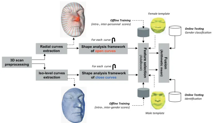
In this work, we combine ideas from shape analysis using tools from differential geometry and feature selection derived from machine learning to select and highlight salient 3D geometrical facial features. After preprocessing of 3D scans, we represent resulting facial surfaces by a finite indexed collections of circular and radial curves. The comparison of pairwise curves, extracted from faces, is based on shape anal-ysis of parameterized curves using differential geometry tools. According to the target application, the extracted features are trained as weak classifiers and the most discriminative features are selected optimally by adaptive boosting. For the case of gender recognition, the classification is formulated as a binary problem (Male/Female classes) and we propose to use the inter- and intra-personal comparisons formulation to achieve feature selection for face identification, which is basically a Multi-class classification problem. Fig. 1 overviews the proposed approach with the target applications, face recog-nition and gender classification. Accordingly, it consists on the following steps:
• The Off-line training step, learns the most salient cir-cular and radial curves from the sets of extracted ones, according to each application in a supervised fashion. In face recognition, for instance, construct feature vectors by comparing pairwise curves extracted from facial surfaces. Next, feed these examples, together with labels indicating if they are inter-class or not. Thus, the adaptive boosting selects and learns iteratively the weak classifiers and adding them to a final strong classifier, with suitable weights. As a result of this step, we keep the T -earliest selected features for the testing step.
• The On-line test step, performs classification of a given test face. In the identity recognition problem, a probe face is compared to the gallery faces using only individual scores computed based on selected features which are fused using the arithmetic mean. In the gender recogni-tion problem, a test face is compared to computed tem-plates of Male and Female classes using curves selected for that purpose. The templates are computed, once for all, within the training stage.
IV. 3DFACIAL CURVES EXTRACTION
Let S be a facial surface denoting the output of a prepro-cessing step that crops the mesh, fills holes, removes noise, and prepares the mesh for curve extraction. We extract radial curves emanating from a reference anchor point (the tip of the nose) and circular curves having with the same point as the pole, using simple procedures detailed in the following paragraphs.
Shape analysis framework of open curves
Shape analysis framework of close curves F e a tu re s e le c tio n (Ad a Bo o s t)
For each curve
3D scan preprocessing Radial curves extraction Iso-level curves extraction F u s io n (A ri th m e ti c m e a n )
For each curve
Offline Training
(intra-, inter-personnal scores)
Online Tes!ng
Iden!fica!on
Offline Training
(intra-, inter-gender scores)
Male template Female template
Online Tes!ng
Gender classifica!on
Fig. 1: Overview of the proposed approach, including both stages of training and testing and both target applications : identity recognition and gender classification.
A. Radial curves
Letβr
αdenote the radial curve onS which makes an angle α with a reference radial curve; the superscript r denotes that it is a radial curve. The reference curve is chosen to be the vertical curve once the face has been rotated to the upright position. In practice, each radial curve βr
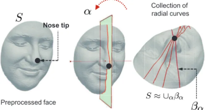
α is obtained by slicing the facial surface by a planePαthat has the nose tip as its origin and makes an angle α with the plane containing the reference curve, as shown in Fig. 3. That is, the intersection of Pα withS gives βr
α. We repeat this step to extract radial curves from the facial surface at equal angular separation. Each curve is indexed by the angle α. To avoid pose variations problem, all probe faces are aligned with the first face model of FRGCv2 database. This step is achieved by performing a coarse alignment by translating the probe face to a reference face, using their noses tips. This coarse alignment step is followed by a fine alignment using the ICP algorithm, as illustrated in Fig. 2.
If needed, we can approximately reconstruct S from these radial curves according to S ≈ ∪αβr
α = ∪α{S ∩ Pα} as illustrated in Figure 3. This indexed collection of radial curves captures the shape of a facial surface and forms the first mathematical representation of that surface.
B. Circular curves
Let βc
λ denote the circular curve on S which makes a distance λ from the reference point (nose tip). A similar procedure is employed to extract these curves. The only difference is the slicing function which is now a sphere Mλ having the reference point as center and variable radiusλ. The
Coarse alignment
First gallery model of FRGCv2
Registration by ICP Fine
alignment
Fig. 2: Probe model pose normalization by registration with the first gallery face of FRGCv2, a coarse alignment is performed by translating the probe face according to the translation vector formed by the tips of the noses. A fine registration is then achieved by the ICP algorithm.
intersection of a given sphere and the facial surface defines equi-distant points from the reference point, in the surface. Fig. 4 illustrates results of such extraction procedure. We note that any points ordering is needed for both kind of curves since the slicing procedure kept edges between points. However, a curve sub-sampling procedure is introduced to achieve the same number of points for all curves (100 points per curve here).
Similarly to radial curves, we can also approximately recon-structS from these circular curves according to S ≈ ∪λβc
λ= ∪λ{S ∩Mλ} as illustrated in Fig. 4, we describe the geometric framework which allow matching and comparison of curves. Fig. 5 gives some results of facial curves extraction on several 3D faces.
Preprocessed face
Collection of radial curves
Nose tip
Fig. 3: Procedure for extraction of radial curves, a curve βr α is obtained by slicing the facial surface byPα defined by the angle α with the vertical plane and having as origin the nose tip.
Preprocessed face Nose tip
Collection of Iso-level curves Sphere with radius =
Fig. 4: Procedure for extraction of circular curves, a curveβc λ is obtained by slicing the facial surface bySλ defined by the radiusλ and having as center the nose tip.
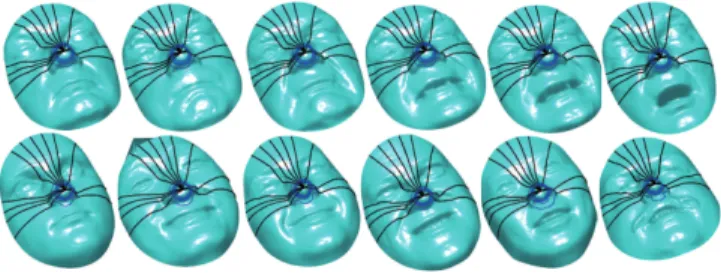
Fig. 5: Examples of facial representation by circular and radial curves. The first row illustrates preprocessed faces of male subjects, the second row gives preprocessed faces of females.
V. GEOMETRIC SHAPE ANALYSIS OF FACIAL CURVES
In the last few years, many approaches have been developed to analyze shapes of 2D curves. We can cite approaches based on Fourier descriptors, moments or the median axis. More recent works in this area consider a formal definition of shape spaces as a Riemannian manifold of infinite dimension on which they can use the classic tools for statistical analysis. The recent results of Michor and Mumford [21], Klassen et al. [10], and Yezzi and Mennucci [22] show the efficiency of this approach for 2D curves. Joshi et al. [23], [24] have recently proposed a generalization of this work to the case of curves defined inRn. We will adopt this work to our problem since our 3D curves are defined in R3.
We start by considering a curve β in R3
. While there are several ways to analyze shapes of curves, an elastic analysis of the parametrized curves is particularly appropriate in our application – face analysis under facial expression variations. This is because (1) such analysis uses the square-root velocity function representation which allows us to compare local facial shapes in presence of elastic deformations, (2) this method uses a square-root representation under which the elastic metric reduces to the standard L2
metric and thus simplifies the analysis, (3) under this metric the Riemannian distance between curves is invariant to the re-parametrization. To analyze the shape ofβ, we shall represent it mathematically using a square-root representation of β as follows ; for an interval I = [0, 1], let β : I −→ R3
be a curve and define q : I −→ R3
to be its square-root velocity function (SRVF), given by:
q(t)=. qβ(t)˙ | ˙β(t)|
(1)
Heret is a parameter ∈ I and | · | is the Euclidean norm in R3. We note that q(t) is a special function that captures the shape of β and is particularly convenient for shape analysis, as we describe next. The classical elastic metric for comparing shapes of curves becomes the L2
-metric under the SRVF representation [24]. This point is very important as it simplifies the calculus of elastic metric to the well-known calculus of functional analysis under theL2
-metric. Also, the squaredL2 -norm of q, given by: kqk2
=R
Ihq(t), q(t)i dt =R k ˙β(t)kdt , is the length ofβ. If we set kqk = 1, implying all curves are rescaled to unit length, then translation and scaling variability have been removed by this mathematical representation of curves.
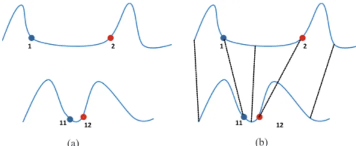
Consider the two curves in Figure 6.a., let us fix the parametrization of the top curve to be arc-length, i.e. traverse that curve with a constant speed equal to one. In order to better match that curve with the bottom one, one should know at what rate we are going to move along the bottom curve so that points reached at the same time on two curves are as close as possible under some geometric criterion. In other words, peaks and valleys should be reached at the same time. Figure 6.b illustrates the matching where point 1 on the top curve matches to point 11 on the bottom curve. The part between the point 1 and 2 on the top curve shrinks on the curve 2. Therefore, the point 2 matches the point 22 on the second curve. An elastic metric is the measure of that shrinking.
A. Radial open curves
The set of all unit-length curves in R3
is given by C = {q : I → R3 |kqk = 1} ⊂ L2 (I, R3 ). With the L2 -metric on its tangent spaces, C becomes a Riemannian manifold. Since the elements ofC have a unit L2
norm,C is a hypersphere in the Hilbert space L2
(I, R3
). In order to compare the shapes of two radial curves, we can compute the distance between them inC under the chosen metric. This distance is found to be the length of the minor arc connecting the two elements inC. Since C is a hypersphere, the formulas for the geodesic
1 2
11 12
1 2
11 12
(a) (b)
Fig. 6: Illustration of elastic metric. In order to compare the two curves in (a), some combination of stretching and bending are needed. The elastic metric measures the amounts of these deformations. The optimal matching between the two curves is illustrated in (b).
and the geodesic length are already well known. The geodesic length between any two points q1, q2∈ C is given by:
dc(q1, q2) = cos−1(hq1, q2i) , (2) and the geodesic pathα : [0, 1] → C, is given by:
α(τ ) = 1
sin(θ)(sin((1 − τ )θ)q1+ sin(θτ )q2) , (3) where θ = dc(q1, q2).
It is easy to see that several elements of C can represent curves with the same shape. For example, if we rotate a face in R3
, and thus its facial curves, we get different SRVFs for the curves but their shapes remain unchanged. Another similar situation arises when a curve is re-parametrized; a re-parameterization changes the SRVF of curve but not its shape. In order to handle this variability, we define orbits of the rotation groupSO(3) and the re-parameterization group Γ as equivalence classes inC. Here, Γ is the set of all orientation-preserving diffeomorphisms ofI (to itself) and the elements of Γ are viewed as re-parameterization functions. For example, for a curve βα : I → R3
and a function γ ∈ Γ, the curve βα◦γ is a re-parameterization of βα. The corresponding SRVF changes according to q(t) 7→ p ˙γ(t)q(γ(t)). We define the equivalent class containing q as:
[q] = {p ˙γ(t)Oq(γ(t))|O ∈ SO(3), γ ∈ Γ} , The set of such equivalence class is called the shape space S of elastic curves [23]. To obtain geodesics and geodesic distances between elements of S, one needs to solve the optimization problem. The resulting shape space is the set of such equivalence classes:
S= C/(SO(3) × Γ). (4)
We denote by ds(βα1, βα2) the geodesic distance between the corresponding equivalence classes [q1] and [q2] in shape space S. In Fig. 7 we show geodesic paths between radial curves and the facial surfaces obtained by Delaunay triangu-lation of the set of points of radial curves. In 7a we show a geodesic path between two facial surfaces of the same person, while in 7b we show the same for faces belonging to different persons.
B. Circular closed curves
We will useβc
λ to denote the circular closed curves. Using SRVF representation as earlier, we can define the set of closed curves inR3 by ˜C = {q : I → R3 |R Iq(t)|q(t)|dt = 0, kqk = 1} ⊂ L2 (I, R3 )}. The quantity R Iq(t)|q(t)|dt is the total displacement inR3
while moving from the origin of the curve until the end. If it is zero, the corresponding curve is closed. Thus, the set ˜C represents the set of all closed curves in R3. It is called a pre-shape space since curves with same shapes but different orientations and re-parameterizations can be represented by different elements of ˜C. To define a shape, its representation should be independent of its rotation and parameterization. This is obtained mathematically by a re-moving the rotation groupSO(3) and the re-parameterization groupΓ from ˜C. As described in [23], [24], we define the orbits of the rotation groupSO(3) and the re-parameterization group Γ as equivalence classes in ˜C. The resulting shape space is :
˜
S= ˜. C/(SO(3) × Γ) (5)
To define geodesics on pre-shape and shape spaces we need a Riemannian metric. For this purpose we inherit the standard L2-metric of the large space L2(I, R3
). For any u, v ∈ L2(I, R3
), the standard L2
inner-product is given by: hhu, vii =
Z
I
hu(t), v(t)i dt . (6) The computation of geodesics and geodesic distances utilize the intrinsic geometries of these spaces. While the detailed description of the geometries of ˜C and ˜S are given in [23], [24], we briefly mention the tangent and normal spaces of ˜C. It can be shown that the set of all functions normal to ˜C at a pointq are given by:
Nq( ˜C) = span{q(t), q i(t)
|q(t)|q(t) + |q(t)|e
i|i = 1, 2, 3} (7)
where {e1
, e2, e3} form an orthonormal basis of R3 . Thus, the tangent space at any point q ∈ ˜C is given by:
Tq( ˜C) = {v : I → R 3
|v ⊥ Nq( ˜C)} (8) Now, an important tool in our framework is the construction of a geodesic path between two elements of ˜S, under the Riemannian metric given by Eq. 6. Given two curvesβc
λ1 and
βc
λ2, represented by their SRVF respectively q1 and q2, we
need to find a geodesic path between the orbits[q1] and [q2] in the space ˜S. We use in this context, a numerical method called the path-straightening method [25] which connects the two points[q1] and [q2] an arbitrary path α and then updates this path repeatedly in the negative direction of the gradient of energy given by:
E[α] = 1 2 Z
s
h ˙α(s), ˙α(s)i ds (9) It has been proven in [25] that the critical points of E defined by Eq. 9 are geodesic paths in ˜S. We denote by d˜s(βλ
1, βλ2) the geodesic distance between the corresponding
equivalence classes [q1] and [q2] in ˜S. In Fig. 8 we show geodesic paths between circular curves and the facial surfaces obtained by Delaunay triangulation of the set of points of
(a) (b)
Fig. 7: 7a shows intra-class geodesics between facial surfaces and their associated radial curves. 7b shows inter-class geodesics between facial surfaces and their associated radial curves.
(a) (b)
Fig. 8: 8a shows intra-class geodesics between facial surfaces and their associated circular curves. 8b shows inter-class geodesics between facial surfaces and their associated circular curves.
circular curves. In 8a we show a geodesic path between two facial surfaces of the same person, while in 8b we show the same for faces belonging to different persons.
C. Extension to facial surfaces shape analysis
In this section we extend our study from shapes of curves to shapes of facial surfaces. We represent the surface of the facial surface S by a collection of 3D circular and radial curves,
S ≈ { Nλ [ λ=1 βλc} ∪ { Nα [ α=1 βαr} , (10) where βc
λ represents the circular curves,Nλ is the cardinality of the set of circular curves,βr
αrepresents the radial curve and Nαis the cardinality of the set of radial curves. Two shapes of facial surfaces are compared by comparing their corresponding facial curves. The distance between two facial surfacesS1
and S2 could be defined by : d(S1 , S2 ) = 1 Nα Nα X α=1 ds(βr,1 α , βαr,2) + 1 Nλ Nλ X λ=1 d˜s(βλc,1, βc,2λ ) (11) VI. BOOSTING FOR GEOMETRIC FEATURE SELECTION
Radial and circular curves capture locally the shape of the faces. However, their comparison under different expressions runs into trouble. In fact, their shapes are affected by changes in facial expressions. For that purposes, we introduce a feature selection step to identify (or localize) the most stable and most discriminative curves. We propose to use the well known machine learning algorithm AdaBoost introduced by Freund
and Schapire in [26]. Recall that, boosting is based on iterative selection of weak classifiers by using a distribution of training samples. At each iteration, the best weak classifier is provided and weighted by the quality of its classification. In practice, the individual circular curves and radial curves are used as weak classifiers. AfterM iterations, the most relevant T (T < M ) facial curves are returned by the algorithm.
A. Face recognition
To train and test Adaboost classifier for this application, we use the 3D face models of FRGCv2 dataset. For each radial and circular curve, we compute the All vs. All (4007 × 4007) similarity matrix. We then split the matrices as we keep the
Gallery vs. Probe of size466×3541 for the testing and uses the remaining Probe vs. Probe sub-matrices, of the size of3541 × 3541, for the training. Thus, we separate the training and the testing samples (the set of individual distances related to facial curves) and these disjoint sets serve as inputs to Adaboost, as illustrated in Fig. 9.
From these areas of the matrices, we extract two kinds of scores (i) the match scores (intra-personal comparisons) and (ii) the non-match scores (inter-personal comparison). Together these scores form an input to the boosting algorithm. More formally, we consider a set of pairs (xk
n, yn)1≤n≤N corresponding to similarity scores between radial or circular curves at the same level, with k = r or k = c. yn can take two values: 0 in the case of non-match score and 1 in the case of match score. For each circular or radial curve, the weak classifier determines the optimal threshold classification function such that the minimum number of samples are misclassified. Each weak classifier hj(xk
n) will take a value of distance computed based on a radial or circular curve,
Match score Non-match score Probe (3541) Gallery Earliest scans (466) Iso-level curves Radial curves Training Tes!ng P ro b e (3 5 4 1 )
Fig. 9: All vs. Probe distance matrices splitting ; the Gallery vs. Probe distance matrix is kept for testing, as suggested in the FRGC evaluation protocol and the remaining sub-matrices
Probe vs. Probe are used for training.
threshold it, and classify the comparison as positive (intra-class) or negative (inter-(intra-class), depending on the distance value being under or over the thresholdθ.
hj(xk n) = ( 1 ifxk n< θ (intra-personal) 0 otherwise. (inter-personal) (12) where, ht denotes for the weak hypothesis given by ht : X → {0, 1}. The final strong classifier is defined by a set of a weak classifiers weighted by a set of weights W = {wt,n}1≤n≤N. The pseudo-code of AdaBoost algorithm is summarized in algorithm 1.
Algorithm 1 AdaBoost algorithm
• Input: A set of samples(xk1, y1), .., (xkN, yN) where xki is the score
of similarity of the circular or radial curves k (1 ≤ k ≤ λ0) and
yn= {0, 1}.
• Let m be the number of non-match score and l be the number of match
score.
Initialisation of weights w1,n=2m1 ,2l1 it depends on the value of yn
where n∈ 1..N . λ0= Nλ+ Nα • For t= 1, ..., M :
1- Normalize the weights wt,nsuch thatPN
n=1wt,n= 1.
2- For each curve βj(feature), train a weak classifier hj that uses
a single curve. The error ǫj of classifier hjis determined with the
corresponding weight wt,1, ..., wt,N: ǫj= N X n wt,n|hj(xjn) − yn|
3- Choose the classifier hjwith the lowest error.
4- Update the weights wt+1,n = wt,nγ1−et n, where γt = 1−ǫǫtt
and en = 0, if the sample xn is correctly classified by ht and 1
else.
• The final hypothesis is a weighted linear combinations of the T
hypotheses where the weights are inversely proportional to the training errors. The strong classifier is given by:
H(x) = ( 1 ifPT t=1logγ1tht(x) ≥ 1 2 PT t=1log(γ1t); 0 else.
The set of selected curves returned by Adaboost is shown in Fig. 10. The first row shows the locations of the selected
curves on different sessions of the same person with different expressions, whereas, the second row gives curves location on different subjects. We note that the boosting algorithm selects iso-curves located on the nasal region, which is stable under expressions and radial curves avoiding two parts. The first one is the lower part of the face since its shape is affected by expressions, particularly when the mouth is open. The second area corresponds to the eye/eyebrow regions. Shapes of radial curves passing throw these regions change when conveying expressions. In contrast, the most stable area cover the nasal/forehead regions.
Fig. 10: The most discriminative radial and circular curves selected by Boosting for face recognition, given on different faces.
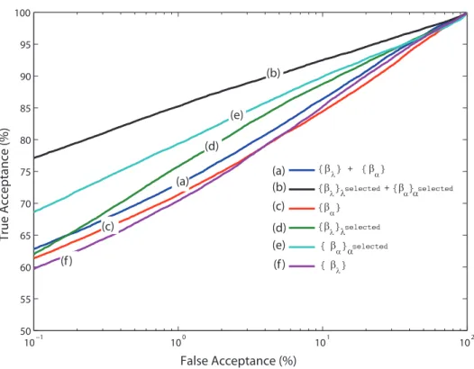
To demonstrate the usefulness of the curve selection step, different graphs in Fig. 11 plot the rate of False Acceptance versus the rate of False Rejection for different configurations. These curves are produced from the Probe vs. Probe matrices (i.e using the training set). As shown in Fig. 11(b), minimum errors are given by fusing scores of selected radial and selected circular curves. We note also that the selection performed on radial curves only or circular curves only minimizes the errors compared to the use of all radial curves or circular curves, respectively.
The on-line testing step consists on comparing faces S1 and S2
by the fusion of scores related to selected curves as following: d(S1 , S2 ) = 1 Nαs Nαs X α=1 ds(βr,1 α , βαr,2) + 1 Nλs Nλs X λ=1 d˜s(βλc,1, βλc,2) (13) where Nλs is the cardinality of the set of selected circular
curves and Nαs the cardinality of the set of selected radial
curves.
B. Gender classification
For 3D face-based gender classification task, we first compute Male and Female representative templates using the geometric shape analysis framework for open and closed curves. In fact, this framework allows us to compute intrinsic means (Karcher mean) of curves that we extend to facial surfaces. Then, within the training step, we compute intra-class (same gender) and inter-intra-class (different gender) pairwise distances (for each curve index) between sample faces and the templates. Finally, the most discriminative geometric features are selected optimally by boosting as done in face
10−1 100 101 102 50 55 60 65 70 75 80 85 90 95 100 False Acceptance (%) True Acceptance (%) {βλ} + { βα} {βλ}λselected + {β α}αselected {βα} {βλ}λselected { βα}αselected { βλ} (b) (e) (d) (a) (c) (f ) (a) (b) (c) (d) (e) (f )
Fig. 11: ROC curves produced from the training set (a) all radial and circular curves (b) selected radial and selected level curves (c) all radial curves (d) selected circular curves (e) selected radial curves (f) all circular curves.
recognition application. For the testing step, distances to male and female templates are computed (based only on selected features), and the nearest neighbor algorithm denotes the class (Male/Female) membership. Different steps are detailed in the following:
Male/Female geometric templates computation. One ad-vantage of the proposed geometrical framework for shape analysis of curves is to calculate some statistics as the "mean" of facial curves and to extend it to facial surfaces, called
Karcher mean [24]. The Riemannian structure defined on a
Riemannian manifold enables us to perform such statistical analysis for computing faces mean and variance. There are at least two ways of defining a mean value for a random variable that takes values on a nonlinear manifold. The first definition, called extrinsic mean, involves embedding the manifold in a larger vector space, computing the Euclidean mean in that space, and then projecting it down to the manifold. The other definition, called the intrinsic mean or the Karcher mean utilizes the intrinsic geometry of the manifold to define and compute a mean on that manifold. It is defined as follows: Let dC(βα
i, βjα) denotes the length of the geodesic path from curves in C. To calculate the Karcher mean of facial curves {βα
1, ..., βnα} in C, we define the variance function:
V : C → R, V(µ) = n X i=1 dC(βα i, βαj) 2 (14) The Karcher mean is then defined by:
βα= arg min
µ∈CV(µ) (15)
The intrinsic mean may not be unique, i.e. there may be a set of points in C for which the minimizer of V is obtained. βα is an element of C that can be seen as the smallest geodesic path length from all given facial surfaces. We present a commonly used algorithm for finding Karcher mean for a given set of facial surfaces (by using their curves). This approach, presented in algorithm 2 uses the gradient of V, in the space Tµ(C), to iteratively update the current mean µ. The same pseudo-algorithm will be obtained for radial curves defined in the shape space ˜C.
Algorithm 2 Karcher mean algorithm
Set k = 0. Choose some time increment ǫ ≤ n1. Choose a point µ0 ∈ C
as an initial guess of the mean. (For example, one could just take µ0 =
S1.)
1- For each i= 1, ..., n choose the tangent vector fi ∈ Tµk(C) which
is tangent to the geodesic from µk to Si. The vector g =Pi=ni=1fi is
proportional to the gradient at µkof the functionV.
2- Flow for time ǫ along the geodesic which starts at µkand has velocity
vector g. Call the point where you end up µk+1.
3- Set k= k + 1 and go to step 1.
Male template facial surface is computed by averaging ten males facial surfaces of different person as shown in Fig. 12. Female template facial surface is computed by averaging ten females facial surfaces of different person as shown in Fig. 13.
Geometric feature selection. To train and test the boosting algorithm for this application, we use 20 previous 3D faces of the FRGCv1 dataset for training and466 subjects of FRGCv2 for testing. Firstly, we selected a subset of faces of men and women (ten from each class) from FRGCv1, to
calcu-(b) Male template face (Karcher mean) (a) Sample faces (from FRGCv1) used
to compute the template face
Fig. 12: Different facial surfaces of different males persons taken from FRGCv1 and their Karcher mean
(b)Female template face (Karcher mean) (a) Sample faces (from FRGCv1)
used to compute the template face
Fig. 13: Different facial surfaces of different females persons taken from FRGCv1and their Karcher mean
late the templates for both male and female classes denoted respectivelyTmaleandTf emale. Then, we computed pairwise distances (based on curves) between test images and both of templates. Thus, we obtained a matrix containing feature vectors (distance based on curves) wich will be used to train Ababoost algorithm, as illustrated in table I. From this matrix, we extract two kinds of scores (i) the match scores (intra-gender comparisons) and (ii) the non-match scores (inter-gender comparison).
TABLE I: Input feature vectors of Boosting algorithm for gender classification.
For each curve Face male1 Face female1 ...
Tmale {xα,λ
n , 1} {xα,λn , 0} ...
Tf emale {xα,λ
n , 0} {xα,λn , 1} ...
Both score lists represent the input of the boosting algorithm. More formally, we consider a set of pairs (xα,λ
n , yn)1≤n≤N wherexα,λn is a similarity score between two curves at the same level α, λ and yn can take two values: 0 in the case of non-match score and 1 in the case of match
score. For each curve βj, the weak learner determines the op-timal threshold classification function, such that the minimum number of samples are misclassified. A weak classifierhj(xk
n) thus consists of a geometric featureβj and a thresholdθ, such that: hj(xk n) = ( 1 if xk n< θ (intra-gender) 0 otherwise. (inter-gender) (16) Fig. 15 shows the location of selected curves on different
Fig. 14: The most discriminative radial and circular curves se-lected by Boosting for gender classification, given on different female faces.
sessions of some male faces whereas, Fig. 14 shows the location of selected curves on different sessions of some female faces.
Fig. 15: The most discriminative radial and circular curves se-lected by Boosting for gender classification, given on different male faces.
We note that the boosting algorithm selects iso-curves on the cheeks region, which is discriminative shape of 3D face for gender classification and radial curves avoiding two parts. The most stable areas for gender classification cover the cheeks/sellion regions.
Classification. As described in table I, this time round, we calculated different matrices of distances of all selected circular and radial curves between template faces and the 466 test faces of FRGCv2. The pseudo-code of the proposed gender classification algorithm is given in algorithm 3.
VII. EXPERIMENTAL RESULTS
In the following, we present conducted experiments and the obtained results with the proposed methods. In particular, we report 3D face recognition performances on FRGCv2 [27] and provide a comparative study with state-of-the-art. FRGCv2 dataset contains 4, 007 3D scans of 466 people, in which more than 40% of the models are non-neutral. A standard evaluation protocol for identification and verification biometric scenarios supports this data set. Furthermore, we give gender classification performances achieved by our approach, using
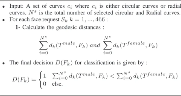
Algorithm 3 Gender classification algorithm
• Input: A set of curves ci where ci is either circular curves or radial
curves. Nsis the total number of selected circular and Radial curves. • For each face request Skk= 1, ..., 466 :
1- Calculate the geodesic distances :
Ns X i=0 dk(Tmale, Fk) and Ns X i=0 dk(Tf emale, Fk)
• The final decision D(Fk) for classification is given by :
D(Fk) = ( 1 PNs i=0dk(Tmale, Fk) <PN s i=0dk(Tf emale, Fk) 0 else.
the same dataset. We note that the subjects in FRGCv2 dataset are 57% male and 43% female.
A. 3D Face Recognition Results
1) Identification: For testing on FRGCv2 dataset, only the
identification evaluation was carried out. In fact, as mentioned in section VI since our approach requires a training stage, it was tested on a subset of this dataset following the FRGC evaluation protocol for the identification scenario, as follow-ing. We kept, for the test, the Gallery vs. Probe (of size 466x3541) similarity matrices. The remaining sub-matrices (i.e Probe vs. Probe similarity scores) were used to train the feature selection step by boosting algorithm. This means that disjointly similarity vectors are used for the training and the test. Following these settings, our approach achieved 98.02% as rank-1 recognition rate and reached 99% in rank-5 as illustrated in the CMC plot (Cumulative Match Characteristic) given by 16. We recall that the approach used here is based on both radial and circular facial curves selection.
2 4 6 8 10 12 14 16 18 20 22 24 26 28 30 98 98.2 98.4 98.6 98.8 99 99.2 99.4 99.6 99.8 RANK Recognition Rate (%)
Fig. 16: The Cumulative Match Characteristic curve for se-lected radial and level curves.
As shown in table II, the selected curves provides better recognition rate that using radial or circular individually. We point out that the most relevant circular curves are located on the nasal region, which means that the nasal shape significantly contribute to face recognition. This is due to to the fact that
TABLE II: Rank-1/Computation cost (in sec) for different configurations.
Performance All Selected
Rank-1 Time(s) Rank-1 Time(s)
Radial 88.65% 1.6 89.04% 0.48
circular 66.51% 1.04 85.65% 0.20
Fusion based on Eq. 13 91.81% 2.64 98.02% 0.68
its shape is stable to facial expressions. We note also that the use combining all the curves by using Eq. 13 provides the best recognition rate.
In addition to performance improvement, the curve selection results on a more compact biometric signature which reduce the time-processing of one-to-one face matching.
2) Comparative study with state-of-the-art: Following the
FRGC standard protocol for the identification scenario, the table III shows identification results of previous approaches (curve-based, feature selection-based, and others) by keeping the earliest scan of the 466 subjects in the gallery and the remaining for testing. We note that experiments reported in [28] and [15] follow a modified protocol by keeping the earliest neutral scan in the gallery and the remaining as test images. It is clear that the proposed method outperforms the majority of state-of-the-art methods. Only the approach proposed recently by Wang et al. [5], based on boosting of descriptors (Haar-like, Gabor, and Local Binary Pattern (LBP)) computed on the Shape Difference Map between faces, achieved a better result98.3% which means that ten more faces are recognized by this approach.
As shown in table III, the proposed approach outperforms the state-of-the-art except the work of [5] .
B. Gender classification
The proposed gender classification of 3D face scans has been experimented using the FRGCv2 database. This was motivated by the fact that this dataset contains the largest number of subjects compared to existing 3D face datasets as Bosphorus, BU-3DFE, etc. To evaluate the proposed approach, we have considered466 3D images related to the 466 subjects of FRGCv2 data set. Thus, if several sessions exist in the dataset, we select the earliest (neutral or non-neutral) one for our experiment. We use also few 3D images taken from FRGCv1 to compute male and female templates, as described in section VI. The difficulty encountered to compare our approach to related work, is there is no standard protocol to compare gender classification results, unlike FRGC standard protocol for 3D face recognition. Most of previous approaches [34],[18],[20] reported classification results on a subset taken from FRGCv1 dataset.
1) Classification results: We conducted experiments by first
computing Male {Tmale} and Female {Tf emale} templates using sample 3D scans taken from FRGCv1. Then, compar-isons between those templates{Tmale, Tf emale} and the 466 test images (of FRGCv2) based on their circular and radial curves were computed to build the feature vectors. Finally, two experiments, detailed below, were carried out:
TABLE III: Comparison with state-of-the-art approaches on FRGCv2 (Rank-1 recognition rate).
Methods
A. Curve-based representation B. Feature selection-based Others
ter Haar Berretti(∗) Mpiperis Drira Faltemier Kakadiaris Wang Huang Mian(∗) Cook
[29] [15] [12] [30] [4] [31] [5] [32] [28] [33]
Rank-1 97% 94.1% - 97.2% 97.2% 97% 98.3% 97.2% 91.9% 92.9%
Our 98.02%
(∗) "E-N-S" means the earliest neutral scan in the gallery and the remaining as probes.
• Experiment 1. Curve selection-based. To select the most
relevant combination of curves using Adaboost algorithm, we first use 10 male 3D face models and 10 female models from FRGCv1 to compute the male and female templates. Then, we compute pairwise curve distances between the same sample models and the templates, in order to build feature vectors, used for the training step. Now, given new test face from the466 3D models of FRGCv2, we compute the pairwise distances to the templates then make the decision as result of the nearest neighbor algorithm. Following this setting, our approach achieved 84.12% as average gender classification rate. We note that, in this experiment, after feature selection step, accumulated distances from selected curves only are used and classification is achieved by nearest neighbor classification. As reported in table IV, we note also that using the combination of selected circular curves and selected radial curves achieved better performances compared to selected circular curves or selected radial curves, taken individually.
TABLE IV: An experimental comparison of gender classifica-tions methods using different types of selected curves.
Methods Curve selection-based 3
circular Radial circular and
curves curves radial curves
Gender Classification Rate 79.40% 80.69% 84.12%
• Experiment 2. Classifier decision-based. In order to
evaluate the boosting classifier results, we have con-ducted, following the same setting, experiments using two machine learning methods, SVM and Neural Network. Instead of feature selection step, we consider the final classifier decision. For example, we consider the binary decision of the strong classifier of Adaboost. Table V summarizes the obtained results. Training and testing steps are carried out using a 10-fold cross-validation experiment. According to this, the466 subjects are splited into disjoint subsets for training and test. Using 10-fold cross validation, training is repeated 10 times, with each of the 10 subsets used exactly once as the test data. Finally, the results from the ten steps are averaged to produce a single estimation of the performance of the classifier for the experiment. In this way, all observations are used for both training and test, and each observation is used for test exactly once.
2) Comparative study with state-of-the-art: Table VI shows
gender classification results compared to previous approaches tested on different subsets. In [35] the authors used a subset of
TABLE V: An experimental comparison of gender classifica-tions methods using different machine learning techniques.
Methods Classifier decision-based
AdaBoost(∗) SVM(∗) Neural(∗)
Network
Gender Classification Rate 86.05% 83.91% 83.05%
(∗) Results for 10-fold cross-validation.
FRGCv1, six female subjects and four male subjects, while in [19] a subset of FRGCv1 is used with only 28 female subjects and 80 male subjects. However they used more than one session of each subject. Note that this ad-hoc division does not guarantee that all subjects will have a neutral expression, some FRGCv2 subjects are scanned with arbitrary facial expression.
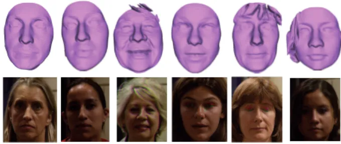
Fig. 17: Different female 3D faces misclassified by our ap-proach. The first row shows 3D data, the second shows the corresponding texture of 3D data.
The analysis of some misclassified examples given by Fig. 17 and 18 shows that there are two major reasons of this misclassification. The first one is the bad quality of 3D scans, such as some occlusions in relevant regions which affected the shape of curves. The second reason lies in the fact that only based on the shape information, there is some confusion (even for a person), to recognize correctly the gender of the person. One solution of this problem and for improving the proposed approach is to introduce the texture information, which contains complementary (as hair density, etc.) in order to consolidate the classifier decision.
The figure 19 shows some faces with selected iso-level and radial curves for both applications face recognition and gender classification, the blue curves are selected for 3-D face gender classification, the red curves are selected for 3-D face recognition while the black curves are the common selected curves for both classifications.
VIII. CONCLUSION
In this paper, by combining tools from Riemannian geome-try and the well-known Adaboost algorithm, we have proposed
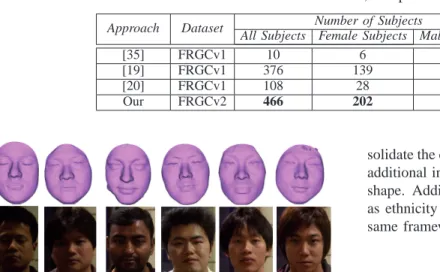
TABLE VI: Gender classification results, comparison to state-of-the-art results.
Approach Dataset Number of Subjects Classification rate
All Subjects Female Subjects Male Subjects
[35] FRGCv1 10 6 4 69.7%
[19] FRGCv1 376 139 237 85.4%
[20] FRGCv1 108 28 80 94.3%
Our FRGCv2 466 202 264 86.05%/84.12%
Fig. 18: Different male 3D faces misclassified by our approach. The first row shows 3D data, the second row shows the corresponding texture of 3D data.
Fig. 19: Examples of selected circular and radial curves for different applications. The first row shows different sessions for different male persons, the second shows different sessions for different female persons.
to select the most discriminative curves for facial recognition and gender classification. The experiments, carried out on FRGCv2 including neutral and non-neutral images, demon-strate the effectiveness of the proposed approach. Based only on 17 curves, including 12 radial curves and 5 circular curves, our fully automatic approach achieved rank-1 recognition rate of 98.02%. For gender classification, 19 curves with 12 radial and 7 circular, were selected and achieved a classification rate of 86.05%. The algorithm computation time was on the order of 0.68 second (for recognition rate) and 0.76 second (for gender classification) to compare two faces with selected curves instead of 2.64 second with all curves. The boosting selects those curves passing through stable regions on the face for different applications. This approach is efficient in terms of computation time, data storage and transmission costs.
The proposed approach can be extended in different direc-tions in order to improve the performances and to address other important classification tasks. For example, the texture information could be associated to shape information to
con-solidate the classifier decision. In fact, texture channel provides additional informations which could be complementary to the shape. Additionally, more facial attributes recognition, such as ethnicity and age estimation could be addressed using the same framework.
ACKNOWLEDGMENT
This research has been supported partialy by the ANR under the projects ANR FAR 3D ANR-07-SESU-004 and the 3D Face Analyzer ANR 2010 INTB 0301 02.
REFERENCES
[1] V. Bruce, A. M. Burton, E. Hanna, P. Healey, O. Mason, A. Coombes, R. Fright, and A. Linney, “Sex discrimination: how do we tell the difference between male and female faces?” Perception, vol. 22, no. 2, pp. 131–52, 1993.
[2] A. J. O’toole, T. Vetter, N. F. Troje, and H. H. Blthoff, “Sex classification is better with three-dimensional head structure than with image intensity information,” Perception, vol. 26, no. 1, pp. 75–84, 1997. [3] F. Daniyal, P. Nair, and A. Cavallaro, “Compact signatures for 3d face recognition under varying expressions,” in Advanced Video and
Signal Based Surveillance, 2009. AVSS ’09. Sixth IEEE International Conference on, sept. 2009, pp. 302–307.
[4] T. C. Faltemier, K. W. Bowyer, and P. J. Flynn, “A region ensemble for 3-d face recognition,” IEEE Transactions on Information Forensics and
Security, vol. 3, no. 1, pp. 62–73, 2008.
[5] Y. Wang, J. Liu, and X. Tang, “Robust 3d face recognition by local shape difference boosting,” IEEE Transactions on Pattern Analysis and
Machine Intelligence, vol. 32, pp. 1858–1870, October 2010.
[6] X. Li, T. Jia, and H. Z. 0002, “Expression-insensitive 3d face recognition using sparse representation,” in CVPR, 2009, pp. 2575–2582. [7] O. Ocegueda, S. K. Shah, and I. A. Kakadiaris, “Which parts of the face
give out your identity?” in CVPR, 2011, pp. 641–648.
[8] H. Li, D. Huang, J.-M. Morvan, and L. Chen, “Learning weighted sparse representation of encoded facial normal information for expression-robust 3d face recognition,” Biometrics, International Joint Conference
on, vol. 0, pp. 1–7, 2011.
[9] C. Samir, A. Srivastava, and M. Daoudi, “Three-dimensional face recognition using shapes of facial curves,” IEEE Transactions on Pattern
Analysis and Machine Intelligence, vol. 28, no. 11, pp. 1847–1857, 2006.
[10] E. Klassen, A. Srivastava, W. Mio, and S. Joshi, “Analysis of planar shapes using geodesic paths on shape spaces,” IEEE Pattern Analysis
and Machine Intelligence, vol. 26, no. 3, pp. 372–383, 2004.
[11] C. Samir, A. Srivastava, M. Daoudi, and E. Klassen, “An intrinsic framework for analysis of facial surfaces,” International Journal of
Computer Vision, vol. 82, no. 1, pp. 80–95, 2009.
[12] I. Mpiperis, S. Malassiotis, and M. G. Strintzis, “3-d face recognition with the geodesic polar representation,” IEEE Transactions on
Informa-tion Forensics and Security, vol. 2, no. 3-2, pp. 537–547, 2007.
[13] H. Drira, B. B. Amor, A. Srivastava, and M. Daoudi, “A riemannian analysis of 3D nose shapes for partial human biometrics,” in IEEE
International Conference on Computer Vision, 2009, pp. 2050–2057.
[14] H. Drira, B. B. Amor, M. Daoudi, and A. Srivastava, “Pose and expression-invariant 3d face recognition using elastic radial curves,” in
BMVC, 2010, pp. 1–11.
[15] S. Berretti, A. D. Bimbo, and P. Pala, “3d face recognition using iso-geodesic stripes,” IEEE Transactions on Pattern Analysis and Machine
Intelligence, vol. 32, no. 12, pp. 2162–2177, 2010.
[16] L. Ballihi, B. B. Amor, M. Daoudi, A. Srivastava, and D. Aboutajdine, “Selecting 3d curves on the nasal surface using adaboost for person authentication,” in 3DOR, 2011, pp. 101–104.
[17] A. M. Burton, V. Bruce, and N. Dench, “What’s the difference be-tween men and women? evidence from facial measurement,”
Percep-tion(London. Print), vol. 22, no. 2, pp. 153–176, 1993.
[18] J. Wu, W. A. P. Smith, and E. R. Hancock, “Facial gender classification using shape from shading and weighted principal geodesic analysis,” in
ICIAR, 2008, pp. 925–934.
[19] X. Lu, H. Chen, and A. K. Jain, “Multimodal facial gender and ethnicity identification,” in ICB, 2006, pp. 554–561.
[20] Y. Hu, J. Yan, and P. Shi, “A fusion-based method for 3d facial gender classification,” in Computer and Automation Engineering (ICCAE), 2010
The 2nd International Conference on, vol. 5, feb. 2010, pp. 369–372.
[21] P. W. Michor and D. Mumford, “Riemannian geometries on spaces of plane curves,” Journal of the European Mathematical Society, vol. 8, pp. 1–48, 2006.
[22] A.-J. Yezzi and A. Mennucci, “Conformal metrics and true "gradient flows" for curves,” in ICCV, vol. 1, 2005, pp. 913–919.
[23] S. H. Joshi, E. Klassen, A. Srivastava, and I. Jermyn, “A novel represen-tation for riemannian analysis of elastic curves in rn,” in CVPR, 2007, pp. 1–7.
[24] A. Srivastava, E. Klassen, S. H. Joshi, and I. H. Jermyn, “Shape analysis of elastic curves in euclidean spaces,” IEEE Transactions on Pattern
Analysis and Machine Intelligence, vol. 33, no. 7, pp. 1415–1428, 2011.
[25] E. Klassen and A. Srivastava, “Geodesics between 3D closed curves using path-straightening,” in Proceedings of ECCV, Lecture Notes in
Computer Science, 2006, pp. I: 95–106.
[26] Y. Freund and R. E. Schapire, “A decision-theoretic generalization of on-line learning and an application to boosting,” in EuroCOLT ’95:
Proceedings of the Second European Conference on Computational Learning Theory. London, UK: Springer-Verlag, 1995, pp. 23–37. [27] P. J. Phillips, P. J. Flynn, W. T. Scruggs, K. W. Bowyer, J. Chang,
K.Hoffman, J. Marques, J. Min, and W. J. Worek, “Overview of the face recognition grand challenge.” in IEEE Computer Vision and Pattern
Recognition, 2005, pp. 947–954.
[28] A. S. Mian, M. Bennamoun, and R. A. Owens, “An efficient multimodal 2d-3d hybrid approach to automatic face recognition,” Pattern Analysis
and Machine Intelligence, IEEE Transactions on, vol. 29, no. 11, pp.
1927–1943, nov. 2007.
[29] F. B. ter Haar and R. C. Veltkamp, “A 3d face matching framework for facial curves,” Graph. Models, vol. 71, no. 2, pp. 77–91, 2009. [30] H. drira, “Statistical computing on manifolds for 3d face
analy-sis and recognition,” Ph.D. dissertation, University Lille 1, 2011, http://www.telecom-lille1.eu/people/drira/dissertation.pdf.
[31] I. A. Kakadiaris, G. Passalis, G. Toderici, M. N. Murtuza, Y. Lu, N. Karampatziakis, and T. Theoharis, “Three-dimensional face recog-nition in the presence of facial expressions: An annotated deformable model approach,” IEEE Transactions on Pattern Analysis and Machine
Intelligence, vol. 29, no. 4, pp. 640–649, 2007.
[32] D. Huang, M. Ardabilian, Y. Wang, and L. Chen, “A novel geometric fa-cial representation based on multi-scale extended local binary patterns,” in Automatic Face Gesture Recognition and Workshops (FG 2011), 2011
IEEE International Conference on, march 2011, pp. 1–7.
[33] J. A. Cook, V. Chandran, and C. B. Fookes, “3d face recognition using log-gabor templates,” in BMVC, Edinborugh, Scotland, 2006, pp. 769– 778.
[34] L. Lu and P. Shi, “A novel fusion-based method for expression-invariant gender classification,” in ICASSP, 2009, pp. 1065–1068.
[35] J. Wu, W. A. P. Smith, and E. R. Hancock, “Gender classification using shape from shading,” in BMVC, UK, 2007, pp. 499–508.
Lahoucine Ballihi received the Master of Advanced
Studies (MAS) degree in Computer science and telecommunications from Mohammed V-Agdal Uni-versity, Faculty of Sciences-Rabat (FSR), Morocco, in 2007 and the Ph.D degree in Computer Science from the University of Lille 1 (USTL), France and the Mohammed V-Agdal University, Rabat, Morocco in 2012. He is also a member of the Computer Science Laboratory in University Lille 1 (LIFL UMR CNRS 8022) and the Computer Science and Telecommunications Research Laboratory of Mo-hammed V-Agdal University, Faculty of Sciences-Rabat (LRIT, unit associated to CNRST (URAC 29)). His research interests are mainly focused on statistical three-dimensional face analysis and recognition and gender classification using 3D images. He is also a teaching assistant in (Telecom Lille1), School of Engineering. Currently, he is a Postdoc within the Computer Science laboratory of the University Lille 1 (LIFL).
Boulbaba Ben Amor received the M.Sc. degree in
2003 and the Ph.D degree in Computer Science in 2006, both from Ecole Centrale de Lyon, France. Currently, he is an associate-professor in Institut Mines-Telecom/Telecom Lille1. He is also a member of the Computer Science Laboratory in University Lille 1 (LIFL UMR CNRS 8022). His research interests are mainly focused on statistical three-dimensional face analysis and recognition and facial expression recognition using 3D. He is co-author of several papers in refereed journals and proceedings of international conferences. He has been involved in French and International projects and has served as program committee member and reviewer for international journals and conferences.
Mohamed Daoudi is Full Professor of Computer
Science at TELECOM Lille 1 and LIFL (UMR CNRS 8022). He is the head of department of Computer Science department at Telecom Lille1. He received the thèse de doctorat degree in Computer Engineering from the University of Lille 1 (USTL), France, in 1993 and Habilitation à Diriger des Recherches from the University of Littoral, France, in 2000. He was the founder and the leader of MIIRE research group http://www-rech.enic.fr/MIIRE/. His research interests include pattern recognition, image processing, three-dimensional analysis and retrieval and 3D face analysis and recognition. He has published over 100 papers in some of the most distinguished scientific journals and international conferences. He is the co-author of the book "3D processing: Compression, Indexing and Watermark-ing ˇT (Wiley, 2008). He was a co-organizer and co-chair of Eurographics 3D Object Retrieval (2009) and ACM Workkshops on 3D Object Retrieval (2010) and Multimedia access to 3D Human Objects MA3HO (2011). He is a senior member of the IEEE.
Anuj Srivastava received the MS and PhD
de-grees in electrical engineering from Washington University, St. Louis, Missouri in 1993 and 1996, respectively. After spending the year 1996-1997 at Brown University as a visiting researcher, he joined FSU as an assistant professor in 1997. He is currently a professor in Department of Statistics at Florida State University (FSU), Tallahassee. His research is focused on pattern theoretic approaches to problems in image analysis, computer vision, and signal processing. In particular, he has developed computational tools for performing statistical inferences on certain nonlinear manifolds, including shape manifolds of curves and surfaces. He has published more than 150 peer-reviewed journal and conference articles in these areas. He is a senior member of the IEEE.
Driss Aboutajdine received the Doctorat de 3ème
Cycle and the Doctorat d’Etat-es-Sciences degrees in signal processing from the Mohammed V-Agdal University, Rabat, Morocco, in 1980 and 1985, re-spectively. He joined Mohammed V-Agdal Univer-sity, Rabat, Morocco, in 1978, first as an assistant professor, then as an associate professor in 1985, and full Professor since 1990, where he is teach-ing, Signal/image Processing and Communications. Over 35 years, he developed teaching and research activities covering various topics of signal and image processing, wireless communication and pattern recognition which allow him to advise more than 50 PhD theses and publish over 200 journal papers and conference communications. He succeeded to found and manage since 1993 and 2001 respectively the LRIT Laboratory and the Centre of Excellence of Information & Communication Technology (pole de competences STIC) which gathers more than 30 research laboratories from all Moroccan universi-ties and including industrial partners as well. Prof. Aboutajdine has organized and chaired several international conferences and workshops. He was elected member of the Moroccan Hassan II Academy of Science and technology on 2006 and fellow of the TWAS academy of sciences on 2007. As IEEE Senior Member, he co-founded the IEEE Morocco Section in 2005 and he is chairing the Signal Processing chapter he founded in December 2010.