RESEARCH OUTPUTS / RÉSULTATS DE RECHERCHE
Author(s) - Auteur(s) :
Publication date - Date de publication :
Permanent link - Permalien :
Rights / License - Licence de droit d’auteur :
Bibliothèque Universitaire Moretus Plantin
Dépôt Institutionnel - Portail de la Recherche
researchportal.unamur.be
University of NamurElastic properties and stability of physisorbed graphene Lambin, Philippe Published in: Applied Sciences DOI: doi:10.3390/app4020282 Publication date: 2014 Document Version
Peer reviewed version
Link to publication
Citation for pulished version (HARVARD):
Lambin, P 2014, 'Elastic properties and stability of physisorbed graphene', Applied Sciences, vol. 4, pp. 282-304. https://doi.org/doi:10.3390/app4020282
General rights
Copyright and moral rights for the publications made accessible in the public portal are retained by the authors and/or other copyright owners and it is a condition of accessing publications that users recognise and abide by the legal requirements associated with these rights. • Users may download and print one copy of any publication from the public portal for the purpose of private study or research. • You may not further distribute the material or use it for any profit-making activity or commercial gain
• You may freely distribute the URL identifying the publication in the public portal ?
Take down policy
If you believe that this document breaches copyright please contact us providing details, and we will remove access to the work immediately and investigate your claim.
applied sciences
ISSN 2076-3417 www.mdpi.com/journal/applsci
Article
Elastic Properties and Stability of Physisorbed Graphene
Philippe Lambin
Physics Department, University of Namur, 61 Rue de Bruxelles, B-5000 Namur, Belgium; E-Mail: philippe.lambin@unamur.be; Tel.: +32-081-724721; Fax: +32-081-724464
Received: 9 March 2014; in revised form: 1 May 2014 / Accepted: 5 May 2014 / Published: 16 May 2014
Abstract: Graphene is an ultimate membrane that mixes both flexibility and mechanical strength, together with many other remarkable properties. A good knowledge of the elastic properties of graphene is prerequisite to any practical application of it in nanoscopic devices. Although this two-dimensional material is only one atom thick, continuous-medium elasticity can be applied as long as the deformations vary slowly on the atomic scale and provided suitable parameters are used. The present paper aims to be a critical review on this topic that does not assume a specific pre-knowledge of graphene physics. The basis for the paper is the classical Kirchhoff-Love plate theory. It demands a few parameters that can be addressed from many points of view and fitted to independent experimental data. The parameters can also be estimated by electronic structure calculations. Although coming from diverse backgrounds, most of the available data provide a rather coherent picture that gives a good degree of confidence in the classical description of graphene elasticity. The theory can than be used to estimate, e.g., the buckling limit of graphene bound to a substrate. It can also predict the size above which a scrolled graphene sheet will never spontaneously unroll in free space.
Keywords: graphite; elasticity; elastic constants; phonons; van der Waals
1. Introduction
According to the European project called GRAPHENE Flagship (http://graphene-flagship.eu/), graphene and related systems are expected to give rise to new materials and devices for information and communications technology, energy saving, and human health improvement at the horizon 2020. This technological revolution will take time: the main applications of graphene are still several years from
now. From a strict fundamental point of view, graphene is a two-dimensional material whose crystalline order cannot survive in free space at the thermodynamic limit (lateral dimensions → ∞) [1]. Both electron diffraction experiments [2] and atomistic calculations [3,4] demonstrate indeed that suspended graphene ripples spontaneously, with typical lateral size between 5 and 10 nm. The situation changes when graphene is deposited on a solid surface, thanks to the interaction with the substrate. Graphite is the best illustration of this effect: its topmost (0001) atomic plane can be very flat, as demonstrated by numerous STM topographical images of highly ordered pyrolytic graphite. However, viewing graphene as a perfect flat sheet on a substrate device can be far from reality [5].
In graphene-based devices, mechanical stress is almost unavoidable. For some applications, this fact cannot be ignored: strain has indeed direct effects on the electronic properties of graphene [6,7]. These effects may become an advantage when used to tailor the transport [8] or other properties. After transfer to a substrate like SiO2, graphene deformation may become important when there is a large amount of
excess material. Wrinkles and folds then form locally [9], which impact the transport properties [5]. Strain also affects the Raman spectra of graphene [10], which is not without consequence given the fact that Raman spectroscopy is widely used in this context as characterization tool. In return, the change of the Raman spectrum induced by strain can be used to measure its characteristics [11,12], provided a quantitative theory of the Raman cross section be available [13,14]. These examples demonstrate how important it is to understand, measure and control the deformation of a graphene overlayer.
Numerous theoretical calculations, either based on empirical potential or on sophisticated ab-initio methods, have been —and still are— performed to study the mechanical properties of graphene (see Section4and reference herein). In parallel, continuous-medium elasticity is applied either to predict or to interpret results of measurements or of computer simulations. It is interesting to point out that many applications of elasticity to graphene and related nanostructures published in the literature are based on the Euler beam theory. The later demands macroscopic parameters such as the thickness of graphene, which is an ambiguous concept [15]. Plate theory is more appropriate to graphene and can be formulated in such a way that it relies on parameters that, non only have a sound physical ground [16], but also can be measured or calculated. Getting the best set of parameters is difficult, however, and far from being completed. On the one hand, experimental measurements of the elastic response of nanostructures by nanomechanics is still challenging (see Section5). On the other hand, “virtual experiments” performed on the computer may lead to scattered data owing to the shape, size and boundary conditions applied to the sample [17].
The present paper aims at formulating the problem of elasticity of graphene within the well-established Kichhoff-Love plate theory, with a clear definition of the few elastic constants it relies on. Without targeting exhaustivity, a critical review of measured and calculated elastic constants is presented. The main result of this review is a comparative table of available data (see Table 1). On this ground, the theory is applied to address the question of stability of graphene upon buckling when it is bound to a flat substrate. A last application is devoted to scrolled graphene, a form that may rapidly becomes more stable than a flat sheet in free space. In any case, one should not forget that continuous-medium elasticity –especially in its linear approximation– has its limits. It is not surprising, then, that breakdown of elasticity has been reported in several instances [18]. The possibility that C has to make bonds of different orders confers to graphene remarkable properties under mechanical
deformation [3], including phase transformation [19]. These questions can only been addressed by atomistic calculations.
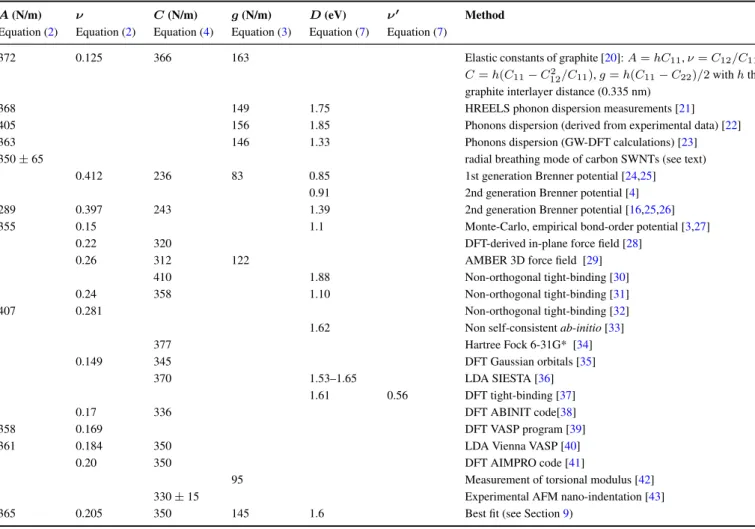
Table 1. Elastic constants of graphene obtained by various methods. Each line of the table lists parameters obtained by independent measurements or calculations.
A (N/m) ν C (N/m) g (N/m) D (eV) ν′ Method Equation (2) Equation (2) Equation (4) Equation (3) Equation (7) Equation (7)
372 0.125 366 163 Elastic constants of graphite [20]: A = hC11, ν = C12/C11,
C = h(C11− C122 /C11), g = h(C11− C22)/2 with h the
graphite interlayer distance (0.335 nm)
368 149 1.75 HREELS phonon dispersion measurements [21]
405 156 1.85 Phonons dispersion (derived from experimental data) [22]
363 146 1.33 Phonons dispersion (GW-DFT calculations) [23]
350± 65 radial breathing mode of carbon SWNTs (see text)
0.412 236 83 0.85 1st generation Brenner potential [24,25]
0.91 2nd generation Brenner potential [4]
289 0.397 243 1.39 2nd generation Brenner potential [16,25,26]
355 0.15 1.1 Monte-Carlo, empirical bond-order potential [3,27]
0.22 320 DFT-derived in-plane force field [28]
0.26 312 122 AMBER 3D force field [29]
410 1.88 Non-orthogonal tight-binding [30]
0.24 358 1.10 Non-orthogonal tight-binding [31]
407 0.281 Non-orthogonal tight-binding [32]
1.62 Non self-consistent ab-initio [33]
377 Hartree Fock 6-31G* [34] 0.149 345 DFT Gaussian orbitals [35] 370 1.53–1.65 LDA SIESTA [36] 1.61 0.56 DFT tight-binding [37] 0.17 336 DFT ABINIT code[38] 358 0.169 DFT VASP program [39]
361 0.184 350 LDA Vienna VASP [40]
0.20 350 DFT AIMPRO code [41]
95 Measurement of torsional modulus [42]
330± 15 Experimental AFM nano-indentation [43]
365 0.205 350 145 1.6 Best fit (see Section9)
2. Teachings of Hooke’s Law and the Kirchhoff-Love Theory
Hooke’s law for crystalline graphite, with its hexagonal symmetry, writes [44] σ11 σ22 σ33 σ32 σ13 σ21 = C11 C12 C13 0 0 0 C12 C11 C13 0 0 0 C13 C13 C33 0 0 0 0 0 0 C44 0 0 0 0 0 0 C44 0 0 0 0 0 0 (C11− C22)/2 ϵ11 ϵ22 ϵ33 2ϵ32 2ϵ13 2ϵ21 (1)
Equation (1) relies on five independent elastic constants.
Two sets of experimental values of the elastic constants of graphite are compared in Table2. The older data set [45] was obtained by ultrasonic, sonic resonance, and static test methods applied to pyrolytic graphite. The more recent data set [20] was deduced from the dispersion curves of acoustic phonons of single-crystalline graphite measured by inelastic X-ray scattering experiments.
Table 2. Experimental values of the elastic constants of graphite (all data in GPa).
References C11 C12 C13 C33 C44 C66
Reference [45] 1060(20) 180(20) 15(5) 36.5(10) 0.18–0.35 440(40) Reference [20] 1109(16) 139(36) 0(3) 38.7(7) 5.0(3) 485(10)
The authors of Reference [20] conclude that, although poorly defined, the C13constant is quite close
to zero. Adopting this conclusion as a simplifying assumption allows one to separate Equation (1) in two independent blocks governing the in-plane and out-of-plane components, respectively, of the stress and strain tensors. Let us consider a plate of graphite with (0001) free surfaces and arbitrary thickness
h and integrate the in-plane block of Hooke’s law over the thickness of the plate. One then obtains
constitutive relations between tension components acting on the sides of the plate (γ = hσ, N/m) and strain components (ϵ)
γ11 = A(ϵ11+ νϵ22)
γ22 = A(ϵ22+ νϵ11) (2) γ12 = A(1− ν)ϵ12
where A is the extensional stiffness (N/m) and ν is the in-plane Poisson coefficient. These expressions are valid in any orthogonal basis set tangent to the plate. For some applications, it will be useful to cast the third relation of Equation (2) in the form
γ12 = 2gϵ12with g = A(1− ν)/2 (3)
where g is the in-plane shear stiffness.
Equation (2) is the basis of Kirchhoff-Love linear theory of elastic isotropic plates (see e.g., Reference [39]). When the plate experiences a uniaxial tension γ (say γ11= γ, γ22= 0), the component ϵ of the strain along the stress direction fulfills the elementary Hooke’s law
γ = Cϵ with C = A(1− ν2) (4)
where C (N/m), which will be called in-plane stiffness constant, plays the same role as the Young modulus does for a macroscopic 3D object. In some cases, it is more easy to measure or to calculate C than A.
In Kirchhoff-Love theory, the elastic strain energy accumulated in the plate subject to in-plane deformation is [46] Es = A 2 ∫ ∫ [(ϵ11+ ϵ22)2+ 2(1− ν)(ϵ212− ϵ11ϵ22)] dS (5)
knowing that the strain tensor is related to the in-plane displacement field ⃗u by the usual definition that,
in Cartesian coordinates, writes [16]
ϵij = 1 2( ∂ui ∂xj +∂uj ∂xi + 2 ∑ k=1 ∂uk ∂xi ∂uk ∂xj ) (6)
The last term may be neglected when ⃗u varies slowly with coordinates. The bending energy takes a
similar expression as the strain energy [47]
Eb =
D
2 ∫ ∫
[(κ11+ κ22)2+ 2(1− ν′)(κ212− κ11κ22)] dS (7)
where D is the bending stiffness or flexural rigidity (J) of the plate, κ is the two-dimensional curvature tensor, and ν′is the same Poisson coefficient ν as in Equation (5) (see below). For small deformations,
κij =
∂2ζ ∂xi∂xj
(8)
where ζ is the mid-surface displacement of the plate with respect to its planar equilibrium shape. Equations (5) and (7) could simply follow by assuming that the energy is a quadratic form of the deformation (linear-response theory) that must involve invariant scalar expressions of the rank-2 tensors
γ and κ due to the assumed in-plane isotropy.
The hypothesis will now be made that Equations (5)–(7) remain valid for one-atom thick graphene, provided suitable elastic constants are used. From now on, A, D, ν, and ν′ will be assumed to be independent elastic constants, which they are not in the traditional plate theory. In the way this theory was derived, A = hC11, ν = C12/C11 = ν′, and D = Ah2/12. For graphene, one cannot rely on
expressions that involve the thickness h, which is ill defined (see Table 2 in Reference [48]). More precisely stated [47], the thickness for extensional deformation of graphene (mostly controlled by the response of the σ bonds) cannot be the same as the one for bending (the flexural rigidity comes chiefly from the π orbitals). Extending the reasoning a step further, there is no reason on why the same Poisson coefficient should take part in both Equations (5) and (7) for graphene. This is the reason why Equation (7) was written with ν′ instead of ν. A generalization of Equation (7) exists in membrane theory where a new bending constant independent of D, the so-called Gaussian curvature modulus, is substituted for the prefactor D(1− ν′) of the term (κ212− κ11κ22) [37]. The applications that follow are
not sensitive to this refinement, because for all of them deal with deformations of graphene for which the Gaussian curvature dtm κ is zero.
3. Teachings of Phonon Dispersion Laws
The first measurements, by high-resolution electron-energy-loss spectroscopy (HREELS), of phonon dispersion curves of graphene on various substrates date back to the years 1980’s (see Reference [49] for a review). The elastic properties of graphene can be obtained from phonon dispersion measurements [21]. The dispersion curves of acoustic phonons in graphene are indeed directly related to its elastic constants and to its mass per unit area µ. The later parameter is a well-defined quantity, which we take as 0.761 mg/m2 (lattice parameter a = 0.246 nm). The long-wavelength velocities of
the longitudinal acoustic (LA) and transverse acoustic (TA) phonons, whose polarization lies inside the graphene plane, can be derived from Equation (5) as follows. The flat plate is supposed to be deformed by a two-dimensional wave ⃗u whose polarization is parallel to the plate. A small perturbation δ⃗u of
identified with a virtual work δEs =−
∫ ∫ ⃗
F · δ⃗u dS. Here, ⃗F is the restoring elastic force per area unit.
Equation (5) together with Equation (6) cleaned from its nonlinear term yield
⃗
F = A ⃗∇⃗∇ · ⃗u − g ⃗∇ × ⃗∇ × ⃗u (9)
where A and g are the extensional stiffness and the in-plane shear stiffness, respectively, introduced above. With that expression, Newton’s law µdS ¨⃗u = ⃗F dS takes the form of a wave equation for ⃗u. That
equation can further be separated in longitudinal ( ⃗∇ × ⃗u = 0) and transverse (⃗∇ · ⃗u = 0) components, with respective phase velocities
cl =
√
A/µ and ct=
√
g/µ (10)
These in-plane elastic wave velocities can be obtained by measuring the slope of the LA and TA phonons at the Γ point. In complement to the work of Reference [21], based on HREELS measurements of the phonon dispersion in CVD (chemical vapor deposition) graphene on Pt(111), two approaches have been followed hereafter. First, a semi-empirical phonon band structure of graphene [22] based on force constants fitted to experimental inelastic X-ray scattering data of graphite [50]. Second, a theoretical
ab-initio phonon band structure of graphene obtained by GW-DFT [23]. The elastic wave velocities obtained by these two approaches are compared in Table3.
Table 3.Slopes ctand clof the TA and LA phonons of graphene at the Γ point and quadratic
coefficient α of the ZA phonon.
ct (km/s) cl (km/s) α (m2/s) Phonon band structure
14.0 22.0 6.1× 10⁻⁷ HREELS measurements [21] 14.3 23.1 6.25× 10⁻⁷ semi-experimental [22] 13.8 21.8 5.28× 10⁻⁷ ab-initio calculations [23]
Out-of plane oscillations of an elastic plate lead to flexural waves. In a similar way as for Equation (9), virtual-work theory can be used to deduce the expression of the elastic forces from the bending energy (Equation (7)) of the plate. For the particular case of a plane wave with small amplitude ζ(x, t) traveling along an arbitrary direction x, the flexural-wave equation is
µ∂ 2ζ ∂t2 + D
∂4ζ
∂x4 = 0 (11)
which imposes a quadratic dispersion relation ωZA = αk2 versus wave vector k, with α =
√
D/µ.
Parabolic fitting of the dispersion curve of the out-of-plane acoustical (ZA) phonon of graphene close to the Γ point gives the values listed in Table3for the band structures referred to above. From the data of Table3, the elastic parameter A, g, and D can be obtained. Their values are listed in Table1.
The radial breathing mode (RBM) of single-walled carbon nanotubes (SWNT) provides us with important piece of information on the elastic properties of the rolled-up graphene sheet. Its real advantage is that it can be measured accurately in resonant Raman spectroscopy. In cylindrical geometry, the x1 and x2 directions referred to in Equation (5) can be taken along the local circumferential and the
strains the nanotube along its circumference, without changing its length and shape. One can therefore set ϵ11= δR/R, ϵ22= ϵ12 = 0 in Equation (5). Accordingly, energy conservation applied to a portion of
length L of the nanotube yields
1 22πRLµ( ˙δR) 2 + A 2 2πRLϵ 2 11 = E (12)
By analogy with the expression of the total energy of an harmonic oscillator, the frequency of the RBM can be deduced: ωRBM = cl/R where cl is the in-plane longitudinal wave velocity given by
Equation (10).
It has been found experimentally that ωRBM = a/d + b, d = 2R being the diameter of the
nanotube. For typical bundles of SWNTs in the diameter range d = 1.5 ± 0.2 nm, a = 234 cm−1 nm and b = 10 cm−1 [51]. For isolated SWNTs on an oxidized Si substrate [52], a = 248 cm−1 nm and
b = 0. Measurement of the RBM for well-identified, free-standing nanotubes gave a = 204 cm−1 nm and b = 27 cm−1 [53]. The last two experiments lead to cl = 23.4 km/s and 19.2 km/s, respectively.
Other measurements realized on long suspended nanotubes with diameter in the range (2.13, 3.82) nm yielded a = 228 ± 1 cm−1 nm and b = 0 [54], which corresponds to a somewhat intermediate value of the longitudinal velocity cl= 21.5 km/s. The corresponding value of the extensional stiffness A is given
in Table 1.
4. Results of Calculations
The calculation of elastic constants of graphene by empirical force-field method and ab-initio technique often proceeds via total-energy calculation of deformed graphene and fitting of the results with Equations (5) or (7). The first calculations date back to the period that followed the discovery of carbon nanotubes [24,33]. According to Equation (5) a longitudinal tensile or compressive axial strain ϵ increases the energy of a single-walled nanotube by ∆E/S = (C/2)ϵ2 where C is the stiffness
constant (Equation (4)) and S is the lateral surface of the rolled up graphene sheet [30]. At that time, graphene was considered by reference with the limiting case of infinite tube radius. Non-orthogonal tight-binding calculations yielded C = 410 N/m [30], slightly more than the results of pseudopotential LDA calculations, C = 370 N/m (60 eV/atom) [36]. Since then, there have been many atomistic calculations specifically devoted to the elastic properties of graphene [28]. The results depend on the specific microscopic model used (see Table 1) and on the type of boundary conditions applied [17]. When calculations are performed on a finite-size graphene sample, the Young modulus is found to be size dependent: below 3nm, the Young modulus decreases by∼10% per each nm reduction [55].
Total-energy calculations of graphene also gives access to the two-dimensional bulk modulus B through the relation ∆E = (B/2) (∆S/S)2, with ∆S the change of the unit-cell area S obtained by
an assumed hydrostatic tension. According to Equation (5), B = A(1 + ν)/2. Published values of B computed by empirical potentials are 200 N/m, typically [27,28], whereas ab-initio VASP calculations yield B = 180 N/m [19].
The in-plane shear stiffness g can be calculated directly from its definition (Equation (3)). To obtain this parameter, a rectangular unit cell of graphene with zigzag and armchair edges is deformed by in-plane shear tensions applied along the four edges. (Note: The honeycomb structure of graphene has
two special directions, orthogonal to each other, qualified as zigzag and armchair. These names come from the shape of the chains of first-neighbor C atoms aligned along these directions. In Figure 1, the tension γ is applied on zigzag edges and is parallel to the armchair direction.) The AMBER molecular mechanics model yields g = 122 N/m [29]. Alternatively, a parabolic fit of the strain energy ∆E/S = (g/2) β2 versus the shear angle β can be used to obtain g. First-generation Brenner potential gives g = 83 N/m [15,25]. Some authors apply a shear along two opposite edges, letting the other two edges free while preventing the free rotation of the graphene sheet [56]. The shear stiffness calculated in this way depends strongly on whether the shear is applied along the zigzag or the armchair edges [28,56].
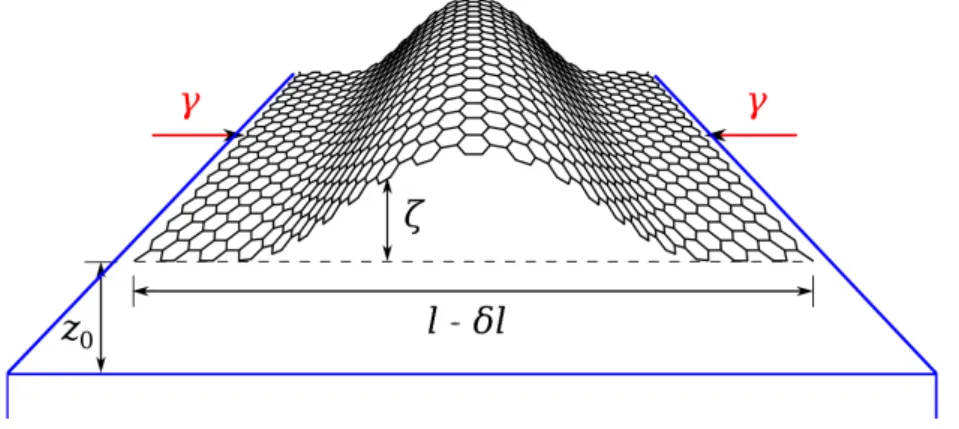
Figure 1. Geometry of buckling for a graphene ribbon of width l physisorbed on a substrate at the equilibrium distance z0. The two edges of the ribbon, supposed to be clamped, are
submitted to a normal tension γ uniformly distributed along the length.
The nanotubes are ideal objects to deal with for calculating the bending stiffness D of graphene. According to Equation (7), rolling up a sheet of graphene for making a nanotube of radius R costs an elastic energy ∆E/S = (D/2) R−2 [24,33]. This penalty is offset by the covalent bonds closing the lateral surface of the tube [57]. Typically, the value of D obtained is 1.6 eV (see Table1).
It is interesting to observe in Table 1 that the elastic constants of graphene calculated with the widely-used Brenner bond-order potential [25] deviate significantly from tight-binding and DFT data. The contribution of dihedral angles in the bond-order coefficient of the interatomic potential of the second generation [58], not present in the original formulation [59], raises the bending stiffness D from 0.8 to 1.4 eV [26].
5. Experimental Nanomechanical Measurements
It is virtually impossible to measure the elastic constants of a single layer graphene via a direct tensile test experiment. One has to proceed indirectly, e.g., by measuring the response of graphene to bending or to torsion.
Reference [42] reports on the frequency shift of a torsional eigenmode of a mechanical oscillator upon deposition of a graphene monolayer on an area called “the neck”. The frequency shift traduces a modification of the torsional rigidity of the oscillator due to the addition of graphene. The torsional
rigidity depends on the shear modulus G of the material (Si) the oscillator is made of and on the shear stiffness g of the graphene overlayer. The relative change of resonance frequency is [42]
∆f
f =
3gθ
2Gt (13)
where t is the thickness of the device (0.3 mm), θ is the fraction of the neck surface covered by graphene and determined by microscopy. Although of the order of 10−5, ∆f /f can be measured, which leads to the value of g given in Table1.
Almost all the published experimental measurements of the Young modulus of graphene are based on AFM nano-indentation realized at the center of graphene suspended above a trench [60,61] or a hole [43,62]. Measuring the slope of the load–displacement curve gives access to the elastic constants of graphene. However, there is always some in-plane residual tension γr in the deposited graphene layer,
which introduces an additional parameter to be fitted along with the elastic constants [60]. For the case of a clamped circular membrane of radius R loaded by a central point force F , Lee et al. [62] proposed the following load–displacement behavior
F = πγrδ + 0.24Cδ3/R2 (14)
where C is the in-plane stiffness constant (Equation (4)) and δ is the AFM tip displacement. Unfortunately, the numerical constant 0.24 depends on the Poisson ratio ν, making the determination of C dependent on the adopted value of ν (taken as 0.165 in Reference [62]). The most recent measured stiffness constant C of graphene is C = 330 ± 15 N/m, irrespective of whether the sample is pristine (exfoliated), large-grain or small grain CVD materials [43]. It has been confirmed by molecular dynamics that the presence of grain boundaries does not reduce significantly the value of C compared to perfect graphene [63,64,65]. However, the mechanical strength (mechanical tension leading to fracture) of samples with average grain sizes 1–5 m is smaller that that of single-crystal graphene, but still retains 85% of the strength of a defect-free sample (33 N/m against 34.5 N/m) [43].
6. Buckling Instability
Buckling will be illustrated here for the case of a graphene ribbon physisorbed on a flat substrate, see Figure1. The equations will be derived by assuming a double-clamp geometry and uniform loads applied along the width l of the ribbon, chosen as x direction. The graphene–substrate interaction potential per unit area is denoted by V . In the continuous medium approximation used throughout this paper, there is no atomic corrugation, with the result that V is a function of the height z above the substrate only. Polymers are well beyond the framework of this approach. They present complex, possibly wavy, surface structures that may influence the geometrical shape of the of the adsorbed graphene depending on the interfacial energy [46]. Investigating the mechanical property of a polymer/graphene interface, where the polymer chains can change their geometry to accommodate the deposited graphene layer, requires sophisticated atomistic calculations [66,67].
For small load, the ribbon accumulates strain energy. Once buckling has taken place, strain becomes negligible compared to bending. The total energy per unit length, including the work done by the external tension γ [68,69], is W = ∫ l 0 [D 2κ 2 + V (z)] ds− γδl = V (z0)l + 1 2 ∫ l 0 [D(d 2ζ dx2) 2 + Kζ2− γ(dζ dx) 2 ] dx (15)
with ds a length element along the width of the deformed ribbon, κ is the local curvature (see Equation (7)), and δl is the shortening of the distance between the anchor points of the forces (see Figure 1). The expression in the most right-hand side of Equation (15) is an approximation valid for small values of the deformation ζ = z − z0 (see Equation (8)), z0 being the equilibrium distance of the
graphene plane above the substrate surface, and K is the second derivative of V (z) at z0.
The deformation ζ is the one that minimizes the energy W . The Euler-Lagrange equation derived from the right-hand side of Equation (15) is the fourth-order differential equation
Dd 4ζ dx4 + γ
d2ζ
dx2 + Kζ = 0 (16)
whose boundary conditions are either imposed values of ζ and dζ/dx at x = 0 and x = l or periodic boundary conditions for ζ and its first three derivatives over the interval l. The critical load is the smallest value of the tension γ for which Equation (16) admits a non trivial solution. In free space (K = 0), a non-zero solution for the double-clamp geometry exists when γ reaches the critical value 4π2D/l2 [16,70]. This solution, ζ(x) = A sin2(πx/l), has even symmetry with respect to mid width. The shape of the buckled sheet of graphene is illustrated in Figure1.
When K ̸= 0, still for the double-clamp geometry of a graphene ribbon of width l (Figure 1), non-trivial solutions of Equation (16) can only exist for γ > 2√DK. The differential equation depends
on two dimensionless parameters, γl2/D and Kl4/D. The relationship between these two parameters is
displayed in Figure2, where the two curves correspond to the “ground state” solutions of Equation (16) that are symmetric and antisymmetric, respectively, with respect to the mid point between the two edges. In both cases, the substrate interaction stabilizes the ribbon against buckling. Interestingly, the difference between the critical tensions for the even and odd symmetries, which is important in the absence of substrate (K = 0), rapidly dims as the force constant of the substrate interaction increases. In some ranges of the parameters, the critical load for the antisymmetric solution comes below the one of the symmetric mode. In the abscissa interval [0.7× 10⁴, 5× 10⁴] the average of the two curves is well fitted
by the expression γl2/D = 4.2154 (Kl4/D)0.4384. In other words the critical bucking tension becomes
almost independent of the ribbon width l, at least in this range of parameter. As shown in Figure 2, the curve γ = 2√DK underestimates by ∼10% the critical load and is indeed independent on the
ribbon width.
To estimate the force constant K of the interaction potential, one may again have recourse to phonon dispersion curves. When the graphene plane is bound to a medium by an assumed harmonic potential, the flexural wave equation introduced here above for a free-standing plate (Equation (11)) is modified in
µ∂ 2ζ ∂t2 + D
∂4ζ
∂x4 + Kζ = 0 (17)
The effects of the restoring force−Kζ imposed by the substrate is to shift the square of the flexural wave frequency ω2by the quantity K/µ. In other words, the frequency of the ZA phonon of graphene at the Γ
point is raised from 0 to√K/µ when it is adsorbed on a substrate. Ab-initio calculations of the phonon
band structure of graphene bound to several metallic surfaces are available [71,72], making it possible to evaluate the force constant K. Results are given in Table 4. The specificity of Cu as substrate for CVD growth of graphene is immediately perceived from the low value of K it leads to. Not only is the force constant weak for graphene on Cu(111), but also the adhesion energy is small: 68 meV/atom according to recent RPA calculations [73] or 120 meV/atom according to nano-mechanical measurement [74]. The force constant for the interaction of graphene on SiO2 has been deduced from semi-empirical energy
calculations of the interface adhesion energy of graphene and few-layer graphite [75]. For graphene on graphite and for graphene on h-BN, the force constant K listed in Table 4 has been obtained by the method described in the Appendix.
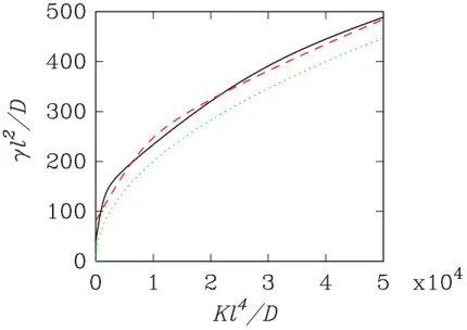
Figure 2. The homogeneous differential equation (Equation (16)) has non trivial solutions for values of the parameters outside the convex side of the curve γ = 2√DK (dotted line).
The figure illustrates the relationship between the equation parameters for the fundamental bucking modes of even (solid-line curve) and odd (dashed-line curve) symmetries when the graphene ribbon is clamped along its two edges distant of l. The value of the critical tension at K = 0 are 39.48 D/l2 and 80.76 D/l2 for the symmetric and antisymmetric
modes, respectively.
Under special preparation techniques, such as liquid exfoliation of graphite, graphene can be strained. A compressive strain may lead to a periodic buckling of the sheet, which will therefore present a regular pattern of ripples. Equation (16) possesses periodic solutions of the type ζ = α cos(kx) + β sin(kx) provided γ = Dk2+ K/k2. γ is the uniaxial tension in the sheet just before it buckles. The minimum
of the last expression, realized for k = √4
K/D, is the critical load for rippling, γcr = 2
√
DK. This
parameter is listed in the fourth column of Table4. The wavelength of the rippled solution is given in the fifth column of the same table. Just before buckling, the strain of the graphene sheet can be estimated by Hooke’s law (Equation (4)). The critical strain is therefore ϵcr = 2
√
DK/C. This parameter is listed
in the last column of Table 4. Remarks that ϵcr vanishes at the limit K → 0, which agrees with the
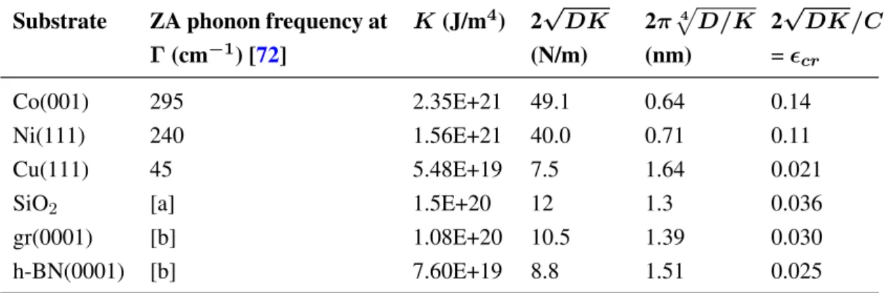
Table 4. Force constant of the the graphene–substrate interaction K and related parameters (see text). The values used for the flexural rigidity D and the stiffness constant C of graphene are 1.6 eV and 350 N/m, respectively.
Substrate ZA phonon frequency at
Γ (cm−1) [72] K (J/m4) 2√DK (N/m) 2π√4 D/K (nm) 2√DK/C = ϵcr Co(001) 295 2.35E+21 49.1 0.64 0.14 Ni(111) 240 1.56E+21 40.0 0.71 0.11 Cu(111) 45 5.48E+19 7.5 1.64 0.021
SiO2 [a] 1.5E+20 12 1.3 0.036
gr(0001) [b] 1.08E+20 10.5 1.39 0.030
h-BN(0001) [b] 7.60E+19 8.8 1.51 0.025
a: see text and Reference [75]; b: see text and Appendix.
It is interesting to point out that periodic, short-wavelength buckling have been observed by high-resolution transmission electron microscopy (TEM) in the top layer of a bi-layer graphite (λ = 0.64 nm) and in a folded graphene sheet near the folding edge (λ = 0.36 nm) [76]. The corresponding observed strains were 0.047 and 0.14, respectively. These values lie above the critical strain predicted for rippling graphene on graphite, 0.03 (see Table4).
When graphene is produced by thermal CVD on a Cu foil, strain comes from the difference of the thermal expansion coefficients of graphene and its substrate. If the graphene overlayer is assumed to be pinned on the substrate, cooling down the graphene/Cu system from 1000 C to room temperature may lead to a uniform compressive strain ϵ of 2.2% [18]. This is very close to the estimated critical strain for rippling on Cu (see Table 4). In those parts of the surface where graphene is not bound to the substrate, ripples may form because of the disappearance of the restoring force from the substrate. Ripples have been observed on graphene suspended over nanotrenches on Cu(111) [18]. These nanotrenches have a width of 5 nm, typically, with length about 10 times bigger. It is interesting that the wavelength of the observed ripples is almost invariably 0.7 nm, the amplitude being ∼0.05nm. These observations cannot be explained by the classical theory of wrinkles that form in a stretched membrane strip with free edges [77]. This should not come as a real surprise. Ripples with wavelength at subnanometer scale are influenced by the atomic structure of graphene much more than by continuum mechanics rules [76]. Independent of all elastic properties, if the residual strain is locally released by ripples that develop above the suspended parts of graphene, then ϵ = (L− λ)/L [78]. In this relation, L is the length measured along the wavy shape of graphene whose projection corresponds to the measured wavelength λ. For a sine function with amplitude a, this expression takes the explicit form
ϵ = 1− π
2E [−(2πa/λ)2] (18)
where E(m) is the complete elliptic integral of the second kind (Equation 17.3.4 in [79]). Accordingly, a strain of 2.2% yields a/λ = 0.048, about 2/3 of the observed ratio. The observed ratio would require a strain of 4.6%. The amplitude and wavelength predicted by atomistic calculations for graphene submitted to a 2.2% compressive edge strain are 0.35 nm and 6.58 nm, respectively [80]. The corresponding a/λ
ratio is 0.053, close to what the above equation yields. However, the amplitude and wavelength of the ripples are an order of magnitude larger than the experimental values. Clearly, not everything is understood here.
To close the discussion, it is instructive to remark that the tension 2Bϵ linked to a uniform strain of 2.2%, where B is the bulk modulus of graphene (see Section 4), is well above the ordinate at K = 0 of the full-line curve of Figure 2. The graphene sheet should therefore buckle across the width of the trench, which is not observed experimentally. Possibly, the ripples that develop along the length of the trench increase considerably the bending stiffness of graphene in the transverse direction, preventing it to buckle, like in a macroscopic corrugated sheet.
7. A Buckling Mode of Non-Supported Graphene: Scrolling
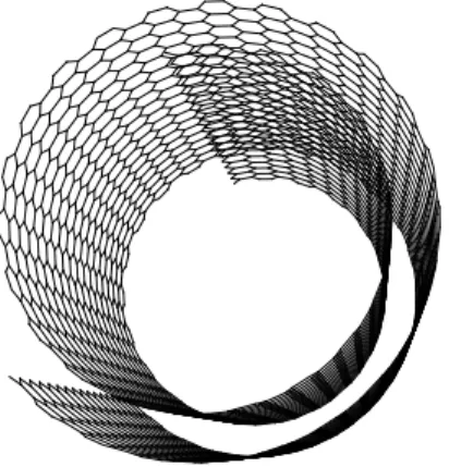
Scrolling a sheet of graphene has a penalty, namely the elastic energy cost to bend the plane. By scrolling graphene, however, the interlayer van der Waals energy of graphite is recovered for these parts of the scrolled sheet that overlap. When the van der Waals interaction exceeds the elastic energy, the scrolled structure may be stable in free space [4]. The very same argument explains the formation of collapsed wrinkles and folds of graphene overlayer [5]. The scroll that should be favored is one for which the successive turns are parallel curves with a constant separation distance h equal to that of multiwall carbon nanotubes or turbostratic graphite. The involute of a circle has precisely this property. Its parametric equations are x = α(τ sinτ + cosτ ) and y = α(−τcosτ + sinτ) where τ is a continuous angular parameter and α = h/2π. Figure3illustrates the scroll.
Figure 3. Perspective view of a rolled sheet of graphene of 16 nm length. The curvature radii at the starting and ending edges of the scroll are 1.24 and 1.80 nm, respectively.
The length of the scroll is l = α(τ22− τ12)/2 where τ1 and τ2 correspond to the inner and outer ends.
The bending energy per unit depth along the z axis can be computed analytically from Equation (7) and set in the form
Eb = D 4α [ F (τ22)− F (τ12)] where F (τ2) = ln(1 + τ2)− τ 2(3τ2+ 2) 2(1 + τ2) (19)
The inner part of the scroll that is surrounded by an outer layer is delimited by τ = τ1 and τ = τ2− 2π.
The total energy per unit depth is [4] Et = Eb − σα[(τ2 − 2π)2 − τ12]/2 where σ is the basal plane
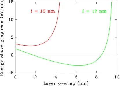
Figure 4. Total energy per depth unit above that of flat graphene of a scrolled sheet such as displayed in Figure3as a function of the length of the overlapping part. The two curves correspond to a sheet of length l of 10 and 17 nm, respectively.
The necessary condition for scrolling is to obtain a negative value of that energy. Noticing that the
elastic bending energy increases logarithmically with the length of the scroll, whereas the van der Waals
energy increases linearly with l, one easily realizes that there is a minimum value of l above which the stability condition can be fulfilled. With the parameter set D = 1.6 eV and σ = 0.21 J/m2 (35 meV/atom) calculated for turbostratic graphite [81], one obtains lmin= 13.5 nm. When the length exceeds that value,
one has to minimize the total energy with respect to τ1 and τ2, while keeping the length constant. The
optimum parameters of the scroll are obtained thereby. Figure4shows the result obtained for a graphene sheet of length equal to 10 nm, for which the scroll is unstable, and for a sheet of length 17 nm, for which the scroll should be stable against unfolding. In the latter case, the optimum geometry corresponds to an overlap of 6.2 nm between the layers.
8. Nonlocal, Nonlinear and Temperature Effects
When the deformations vary on a length scale that is not much larger than atomic distances, it is possible to extend the domain of validity of elasticity by turning to a nonlocal response of the material [82]. In the particular case of graphene, nonlocal elasticity consists chiefly in replacing each component of the algebraic Hooke’s law (Equation (2)) by a differential equation of the kind
(1− ξ2∆)γ11= A (ϵ11+ νϵ22) (20)
(∆ is the Laplacian) and similar equations for γ12and γ22. In that relation, ξ is a non-locality parameter,
which is of the order of the interatomic distances. For an unbounded graphene plane, a formal solution of Equation (20) writes γ11(x1, x2) = 1 2πξ2 ∫ ∫ A [ϵ11(x′1, x′2)+νϵ22(x′1, x′2)] K0( √ (x′1− x1)2+ (x′2− x2)2/ξ) dx′1dx′2 (21)
where K0 is the modified Bessel function of the second kind and order 0. In nonlocal elasticity, the
tension at the reference point (x1, x2) depends on the strain field everywhere, the dependency decreasing
exponentially with the distance to the reference point measured in units of ξ.
When this theory is used to study in-plane elastic waves in graphene, the effect of non locality on Newton’s law consists in the substitution of (1− ξ2∆)¨⃗u for the acceleration ¨⃗u, without modification of
the expression of the restoring elastic force (Equation (9)) [83]. As the result, the dispersion relation for plane waves now takes the form
ω = √ ck
1 + ξ2k2 (22)
with k the modulus of the two dimensional wave-vector, where the velocity c denotes cl or ct for the
longitudinal or transverse modes, respectively, with expressions given by Equation (10). The dispersion relation deviates from the strict linear form. When ξk is small, ω ≈ ck(1 − ξ2k2/2). This behavior
is qualitatively correct in the sense that the LA and TA modes of graphene now have a negative dispersion (the phase velocity decreases with increasing k), as indeed observed experimentally [21] and by calculations [23]. If Equation (22) had to reproduce the experimentally-measured frequencies of the TA or LA phonons at the K point of the first Brillouin zone, ξ would take the values 0.044 or 0.077 nm, respectively. Should one want to fit the TA and LA frequencies at the M point, other values of ξ would be obtained. Not only the non-locality parameter depends on the wave polarization, also does it depend on the direction of the wave vector.
In nonlocal elasticity, the equation for flexural waves is transformed along the same way as the one governing in-plane vibrations: the acceleration term in Equation (11) is replaced by µ(1− ξ2∇2)¨ζ [84].
Accordingly, the dispersion relation of the out-of-plane wave now becomes ωZA = αk2/
√
1 + ξ2k2with α =√D/µ as before. A best fit over the first half of the ΓK line of the ZA phonon branch obtained by
GW calculations [23] gives ξ = 0.052 nm. This value is intermediate between the values of ξ deduced from the TA and LA phonon dispersion. In any case, ξ is a small fraction of the CC distance, which raises question on its exact physical meaning.
Within nonlocal elasticity, one-dimensional out-of-plane deformations of graphene bound to a substrate (Equation (16)) are governed by the following equation [85,86]
Dd 4ζ dx4 + γ ( d2ζ dx2 − ξ 2d4ζ dx4) + K (ζ − ξ 2d2ζ dx2) = 0 (23)
Numerical calculations show that the buckling load is reduced compared to the predictions of local elasticity [86,87]. However, this reduction is significant only for graphene ribbons with small width, of the order of ξ. This conclusion can readily be substantiated for the case of a self-supported graphene strip, by setting K=0 in the above equation. For a given applied compressive tension γ, the role of the non-locality parameter is to weaken the bending stiffness to D − ξ2γ. Accordingly, the critical load
triggering the buckling mode illustrated in Figure1is γcr = 4π2D/(l2+ 4π2ξ2). Non locality has little
effects as soon as l ≫ 2πξ ≈ 0.3 nm.
The stability of physisorbed graphene is now briefly revisited in the light of nonlocal elasticity. A rippled solution of Equation (23) with wave vector k requires γ = Dk2/(1 + ξ2k2) + K/k2. The
minimum of that expression is γcr = 2
√
KD− Kξ2 if ξ2 < √D/K or γ
cr = D/ξ2 if ξ2 >
√
D/K.
cases listed in Table4. For Cu and h-BN, a non-locality parameter ξ = 0.05 nm reduces the critical strain given in the last column of Table4by∼ 5 × 10⁻⁴, which is negligible.
Besides non-locality, nonlinear contributions may be worth accounting for when the strain exceeds a few percents, which is not unrealistic in the case of graphene [62]. First of all, the last term in Equation (6) must be kept when dealing with a rapidly varying in-plane displacement field vectu. For strong bending, the simplified expression ∂2ζ/∂xi∂xj of the curvature tensor κij is no longer valid [16].
Second, nonlinear Hooke’s law should be used. For uniaxial tension, in particular, the elementary Hooke’s law (Equation (4)) transforms into
γ = Cϵ + C2ϵ2(plus higher order terms) (24)
The nonlinear response coefficient C2depend on elements of the second- and third-order elastic-constant
tensors generated by Taylor expansion of the elastic energy versus strain [39]. Equation (24) is slightly anisotropic in the sense that the value of C2 depends on the direction of the applied tension γ (C2 = −670 N/m and −700 N/m in the zigzag and armchair directions, respectively, according to ab-initio calculations of Reference [28]). It is worth to mention, however, that in nanoindentation experiments performed on graphene, the nonlinear coefficient C2 plays a role in such a small fraction of
the deformed graphene sheet that its overall effect can be ignored [62].
Temperature affects the elastic properties of any material. In graphene, thermal fluctuations of the out-of-plane displacements are important, at least in self-supported geometry [4]. In the harmonic approximation, the mean square displacement normal to the plane is [3,55]
⟨ζ2⟩ ≈ kBT
D S
30π2 (25)
where kBis the Boltzmann constant and S is the area of the sample. The root mean square displacement
increases therefore like √S and may become important in a large free-standing sample. In direct
connection with the previous Section, atomistic simulations show that the transformation of a graphene nanoribbon into a nanoscroll may happen spontaneously at room temperature when the aspect ratio
l/W is large, thanks to large-amplitude thermal fluctuations [4]. Molecular dynamics calculations show that ⟨ζ2⟩ is not proportional to T , which means that the bending stiffness D is temperature dependent.
Indeed, D increases with temperature [3]. The other elastic constants of graphene also exhibit a peculiar temperature dependence according to atomistic calculations [27,88], although other molecular dynamical studies predict a normal monotonous decrease of the Young modulus with temperature [40,89]
9. Conclusions
The framework of this paper is a continuous-medium plate theory applied to elasticity of a graphene. This theory relies on a few elastic constants that remain well defined at the limit of an atomic monolayer. In particular, there is no need to assign a thickness to graphene. Values of the elastic constants taken from available published data, both theoretical and experimental, are listed in Table1. If one excludes the first row of this table (extrapolation of graphite bulk elastic constants to the monolayer limit) and the data deduced from Brenner potential that deviate significantly from other sources, a rather coherent picture emerges. A least-square fit of the values of the in-plane constants A, ν, C, and g under the constraints
imposed by Equations (3) and (4), yields the value listed in the last row of Table1. Among them, the emblematic Young modulus—actually the in-plane stiffness constant, Equation4—is C = 350 N/m. As for the flexural rigidity, the retained value D = 1.6 eV is the average of the tabulated data, excluding those coming from Brenner potential.
In the last sections of the paper, it has been shown that the interaction of graphene with its substrate strengthens it against buckling instability. When adsorbed on Cu, graphene can sustain a compressive strain slightly above 2% (last column of Table 4), and more on other substrates, without rippling. By comparison, an average compressive strain on the order of 0.5% was determined by Raman spectroscopy in graphene on Cu(111) [12]. Nonlocal generalization of Hooke’s law has been shown to have little effects in graphene, except if the width of the sample is less than 1 nm or if the length scale of the deformation falls below the nanometer. In free space, flat graphene becomes unstable with increasing lateral dimensions. If a graphene sheet scrolls, it will not unroll spontaneously when its length exceed
∼13 nm.
Acknowledgments
The author acknowledges Valentin N. Popov (Sofia) and Ludger Wirtz (Luxemburg) for useful and constructive discussions.
Appendix: Force Constant of the Girifalco Interaction Potential
In this appendix, the energetics of a graphene plane physisorbed on a layered crystal is developed on the basis of the Girifalco potential [90]. In the Girifalco approach, each carbon of the graphene interacts with the atomic planes of the substrate through a 6–12 Lennard-Jones potential C12/r12− C6/r6, the
sums over the atomic pairs being replaced by integrals. The interaction of a C atom with a given atomic plane of the substrate at distance d is
V1(d) = b
10d10 − a
4d4 (26)
The interaction of a C atom with a massive substrate follows by summing Equation (26) over an infinite set of planes parallel to the surface. Assuming a regular inter plane spacing h yields
V (z) = b
10h10ζ10(z/h) − a
4h4 ζ4(z/h) (27)
where z is the distance of graphene above the surface and ζs(x) =
∑∞
n=0(x + n)−s is a generalized
Riemann function (x > 0, s > 1).
For a given substrate, when the parameters a and b are known together with the bulk interlayer spacing
h, the adsorption distance z0 of the graphene plane is obtained by minimizing Equation (27). The
force constant K (Table 4) of the interaction potential is the second derivative of V (z) at equilibrium, multiplied by the number N of C atoms per unit area in graphene.
To obtain the Grifalco parameters for graphite, Equation (27) is applied to a C atom located in the bulk, namely in between two semi-infinite multilayers, while setting z = h. In this geometry, the bulk energy per C atom writes E = B/10h10− A/4h4 where A = a ζ4 and B = b ζ10 with ζs ≡ ζs(1) is the
usual Riemann function. The interlayer distance leading to the minimum of energy is h = (B/A)1/6. A second relation is obtained from the elastic constant C33that corresponds to the second derivative of the
bulk energy per unit volume at the equilibrium distance, which leads to C33 = 6N A/h5. Using the value
of h given in TableA1, N = 38.18 nm−2, and C33= 38.7 GPa (Table2), one obtains A = 4.48 meV nm4
and B = 6.38× 10⁻³ meV nm10. The a and b parameters listed in TableA1follow from the definition of A and B.
Table A1. Girifalco parameters describing the interaction of a C atom with graphite and hexagonal boron nitride (see text)
Substrate h (nm) a (meV nm4) b (meV nm10) z 0(nm)
gr(001) 0.3354 4.14 6.37× 10³ 0.338 h-BN(001) 0.3331 3.25 5.49× 10³ 0.343
For the case of graphene on BN, ab-initio RPA data of graphene on a single BN layer have been used [91]. In this reference, six positions of the graphene layer on top of the BN layer were considered while assuming a common parameter for the two hexagonal lattices. The average potential well and separation distance are 34.5 meV/atom and 0.345 nm, respectively. Fitting Equation (26) on these data leads to the parameters listed in TableA1.
Conflicts of Interest
The author declares no conflict of interest.
References
[1] Mermin, N.D. Crystalline order in two dimensions. Phys. Rev. B 1968, 176, 250–254.
[2] Meyer, J.C.; Geim, A.K.; Katsnelson, M.I.; Novoselov, K.S.; Booth, T.J.; Roth, S. The structure of suspended graphene sheets. Nature 2007, 446, 60–63.
[3] Fasolino, A.; Los, J.H.; Katsnelson, M.I. Intrinsic ripples in graphene. Nat. Mater. 2007, 6, 858–861.
[4] Xu, Z.; Buehler, M. Geometry controls conformation of graphene sheets: Membranes, ribbons, and scrolls. ACS Nano 2010, 4, 3869–3876.
[5] Zhu, W.; Low, T.; Perebeinos, V.; Bol, A.A.; Zhu, Y.; Yan, H.; Tersoff, J.; Avouris, P. Structure and electronic transport in graphene wrinkles. Nano Lett. 2012, 12, 3431–3436.
[6] Farjam, M.; Rai-Tabar, H. Comment on “Band structure engineering of graphene by strain: First-principles calculations”. Phys. Rev. B 2009, 80, 167401.1–167401.3.
[7] Li, Y.; Jiang, X.; Liu, Z.; Liu, Z. Strain effects in graphene and graphene nanoribbons: The underlying mechanism. Nano Res. 2010, 3, 545–556.
[8] Peres, N.M.R. Colloquium: The transport properties of graphene: An introduction. Rev. Mod.
Phys. 2010, 82, 2673–2700.
[9] Liu, N.; Pan, Z.; Fu, L.; Zhang, C.; Dai, B.; Liu, Z. The origin of wrinkles on transferred graphene.
[10] Mohiuddin, T.M.G.; Lombardo, A.; Nair, R.R.; Bonetti, A.; Savini, G.; Jali, R.; Bonini, N.; Basko, D.M.; Galiotis, C.; Marzari, N.; et al. Uniaxial strain in graphene by Raman spetrosopy: G peak splitting, Gruneisen parameters and sample orientation. Phys. Rev. B 2009, 79,
205433.1–205433.8.
[11] Ferralis, N. Probing mechanical properties of graphene with Raman spectroscopy. J. Mater. Sci. 2010, 45, 5135–5149.
[12] He, R.; Zhao, L.; Petrone, N.; Kim, K.S.; Roth, M.; Hone, J.; Kim, P.; Pasupathy, A.; Pinczuk, A. Large physisorption strain in chemical vapor deposition of graphene on copper substrates.
Nano Lett. 2012, 12, 2408–2413.
[13] Frank, O.; Mohr, M.; Maultzsch, J.; Thomsen, C.; Riaz, I.; Jalil, R.; Novoselov, K.S.; Tsoukleri, G.; Parthenios, J.; Papagelis, K.; Kavan, L.; Galiotis, C. Raman 2D-band splitting in graphene: Theory and experiment. ACS Nano 2011, 5, 2231–2239.
[14] Popov, V.N.; Lambin, Ph. Theoretical 2D Raman band of strained graphene. Phys. Rev. B 2013,
87, 155425.1–155425.7.
[15] Huang, Y.; Wu, J.; Hwang, K.C. Thickness of graphene and single-wall carbon nanotubes. Phys.
Rev. B 2006, 74, 245413.1–245413.9.
[16] Lu, Q.; Huang, R. Nonlinear mechanics of single-atomic-layer graphene sheets. Intern. J. Appl.
Mechan. 2009, 1, 443–447.
[17] Maren´c, E.; Ibrahimbegovic, A.; Sori´c, J.; Guidault, P.A. Homogenized elastic properties of graphene for small deformations. Materials 2013, 6, 3764–3782.
[18] Tapaszto, L.; Dumitrica, T.; Kim, S.J.; Nemes-Incze, P.; Hwang, C.; Biro, L.P. Breakdown of continuum mechanics for nanometre-wavelength rippling of graphene. Nat. Phys. 2012, 8, 739–742.
[19] Marianetti, C.A.; Yevick, H.G. Failure mechanisms of graphene under tension. Phys. Rev. Lett. 2010, 105, 245502.1–245502.4.
[20] Bosak, A.; Krisch, M.; Mohr, M.; Maultzsch, J.; Thomsen, C. Elasticity of single-crystalline graphite: Inelastic x-ray scattering study. Phys. Rev. B 2007, 75, 153408.1–153408.4.
[21] Politano, A.; Raimondo Marino, A.; Campi, D.; Far´ıas, D.; Miranda, R.; Chiarello, G. Elastic properties of a macroscopic graphene sample from phonon dispersion measurements. Carbon 2012, 50, 4903–4910.
[22] Michel, K.H.; Verberck, B. Theory of the elastic constants of graphite and graphene. Phys. Stat.
Sol. (b) 2008, 245, 2177–2180.
[23] Lazzeri, M.; Attaccalite, C.; Wirtz, L.; Mauri, F. Impact of the electron-electron correlation on phonon dispersion: Failure of LDA and GGA DFT functionals in graphene and graphite.
Phys. Rev. B 2008, 78, 081406R.1–081406R.4.
[24] Robertson, D.H.; Brenner, D.W.; Mintmire, J.W. Energetics of nanoscale graphitic tubules.
Phys. Rev. B 1992, 45, 12592–12595.
[25] Arroyo, M.; Belytschko, T. Finite crystal elasticity of carbon nanotubes based on the exponential Cauchy-Born rule. Phys. Rev. B 2004, 69, 115415.1–11541511.
[26] Lu, Q.; Arroyo, M.; Huang, R. Elastic bending modulus of monolayer graphene. J. Phys. D 2009,
[27] Zakharchenko, K.V.; Katsnelson, M.I.; Fasolino, A. Finite temperature lattice properties of graphene beyond the quasiharmonic approximation. Phys. Rev. Lett. 2009, 102, 046808.1–046808.4.
[28] Kalosakas, G.; Lathiotakis, N.N.; Galiotis, C.; Papagelis, K. In-plane force fields and elastic properties of graphene. J. Appl. Phys. 2013, 113, 134307.1–134307.7.
[29] Tsai, J.L.; Tu, J.F. Characterizing mechanical properties of graphite using molecular dynamics simulation. Mater. Des. 2010, 31, 194–199.
[30] Hernandez, E.; Goze, C.; Bernier, P.; Rubio, A. Elastic properties of C and BxCyNz composite
nanotubes. Phys. Rev. Lett. 1998, 80, 4502–4505.
[31] Xin, Z.; Jianjun, Z.; Zhong-can, O.Y. Strain energy and Young modulus of single-wall carbon nanotubes calculated from energy-band theory. Phys. Rev. B 2000, 62, 13692–13696.
[32] Popov, V.N. Private communication, 2012.
[33] Adams, G.B.; Sankey, O.F.; Page, J.B.; O’Keeffe, M.; Drabold, D.A. Energetics of large fullerenes: Balls, tubes, and capsules. Science 1992, 256, 1792.
[34] Van Lier, G.; van Alsenoy, C.; van Doren, V.; Geerlings, P. Ab initio study of the elastic properties of single-walled carbon nanotubes and graphene. Chem. Phys. Lett. 2000, 326, 181–185.
[35] Kudin, K.N.; Scuseria, G.E.; Yakobson, B.I. C2F, BN, and C nanoshell elasticity from ab initio
computations. Phys. Rev. B 2001, 64, 235406.1–23540610.
[36] Sanchez-Portal, D.; Artacho, E.; Soler, J.M.; Rubio, A.; Ordejon, P. Ab initio structural, elastic, and vibrational properties of carbon nanotubes. Phys. Rev. B 1999, 59, 12678–12688.
[37] Koskinen, P.; Kit, O.O. Approximate modeling of spherical membranes. Phys. Rev. B 2010, 82, 235420.1–235420.5.
[38] Leenaerts, O.; Peelaers, H.; Hern´andez-Nieves, A.D.; Partoens, B.; Peeters, F.M. First-principles investigation of graphene uoride and graphane. Phys. Rev. B 2010, 82, 195436.1–195436.5. [39] Wei, X.; Fragneaud, B.; Marianetti, C.A.; Kysar, J.W. Nonlinear elastic behavior of graphene:
Ab initio calculations to continuum description. Phys. Rev. B 2009, 80, 205407.1–205407.8.
[40] Shao, T.; Wen, B.; Melnik, R.; Yao, S.; Kawazoe, Y.; Tian, Y. Temperature dependent elastic constants and ultimate strength of graphene and graphyne. J. Chem. Phys. 2012, 137, 194901.1–194901.8.
[41] Wagner, P.; Ivanovskaya, V.V.; Rayson, M.J.; Briddon, P.R.; Ewels, C.P. Mechanical properties of nanosheets and nanotubes investigated using a new geometry independent volume definition.
J. Phys.: Condens. Matter 2013, 25, 155302.1–155302.5.
[42] Liu, X.; Metcalf, T.H.; Robinson, J.T.; Houston, B.H.; Scarpa, F. Shear modulus of monolayer graphene prepared by chemical vapor deposition. Nano Lett. 2012, 12, 1013–1017.
[43] Lee, G.H.; Cooper, R.C.; An, S.J.; Lee, S.; van der Zande, A.; Petrone, N.; Hammerberg, A.G.; Lee, C.; Crawford, B.; Oliver, W.; Kysar, J.W.; Hone, J. High-strength chemical-vapor deposited graphene and grain boundaries. Science 2013, 340, 1073–1076.
[44] Kelly, B.T. Physics of Graphite; Applied Science Publishers: London, UK, 1981; pp. 62–76. [45] Blakslee, O.L.; Proctor, D.G.; Seldin, E.J.; Spence, G.B.; Weng, T. Elastic constants of
[46] Zhang, Z.; Li; T. Determining graphene adhesion via substrate-regulated morphology of graphene.
J. Appl. Phys. 2011, 110, 083526.1–083526.5.
[47] Yakobson, B.I.; Brabec, C.J.; Bernholc, J. Nanomechanic of carbon tubes: Instabilities beyond linear response. Phys. Rev. Lett. 1996, 76, 2511–2514.
[48] Harik, V.M. Mechanics of carbon nanotube: Applicability of the continuum-beam models.
Comput. Mater. Sci. 2002, 24, 328–342.
[49] Oshima, C.; Nagashima, A. Ultra-thin epitaxial films of graphite and hexagonal boron nitride on solid surfaces. J. Phys.: Condens. Matter 1997, 9, 1–20.
[50] Mohr, M.; Maultzsch, J.; Dobard, E.; Reich, S.; Milosevic, I.; Damnjanovic, M.; Bosak, A.; Krisch, M.; Thomsen, C. The phonon dispersion of graphite by inelastic x-ray scattering. Phys. Rev. B 2007, 76, 035439.1–035439.7.
[51] Jorio, A.; Pimenta, M.A.; Filho, A.G.S.; Saito, R.; Dresselhaus, G.; Dresselhaus, M.S. Characterizing carbon nanotube samples with resonance Raman scattering. New J. Phys. 2003, 5, 139.1–139.17.
[52] Jorio, A.; Saito, R.; Hafner, J.H.; Lieber, C.M.; Hunte, M.; McClure, T.; Dresselhaus, G.; Dresselhaus, M.S. Structural (n,m) Determination of Isolated Single-Wall Carbon Nanotubes by Resonant Raman Scattering. Phys. Rev. Lett. 2001, 86, 1118–1121.
[53] Meyer, C.; Paillet, M.; Michel, T.; Moreac, A.; Neumann, A.; Duesberg, G.S.; Roth, S.; Sauvajol, J.L. Raman-modes of index-identified free-standing single-walled carbon nanotubes.
Phys. Rev. Lett. 2005, 95, 217401.1–217401.4.
[54] Liu, K.; Wang, W.; Wu, M.; Xiao, F.; Hong, X.; Aloni, S.; Bai, X.; Wang, E.; Wang, F. Intrinsic radial breathing oscillation in suspended single-walled carbon nanotubes. Phys. Rev. B 2011, 83, 113404.1–113404.4.
[55] Jiang, J.W.; Wang, J.S.; Li, B. Young’s modulus of graphene: A molecular dynamics study.
Phys. Rev. B 2009, 80, 113405.1–1134054.
[56] Min, K.; Aluru, N.R. Mechanical properties of graphene under shear deformation. Appl. Phys.
Lett. 2011, 98, 013113.1–013113.3.
[57] Lucas, A.A.; Lambin, P.; Smalley, R.E. On the energetics of tubular fullerenes. J. Phys. Chem.
Solids 1993, 54, 587–593.
[58] Brenner, D.W.; Shenderova, O.A.; Harrison, J.A.; Stuart, S.J.; Ni, B.; Sinnott, S.B. A second generation reactive empirical bond order (REBO) potential energy expression for hydrocarbons.
J. Phys.: Condens. Matter 2002, 14, 783–802.
[59] Brenner, D.W. Empirical potential for hydrocarbons for use in simulating the chemical vapor deposition of diamond films. Phys. Rev. B 1990, 42, 9458–9471.
[60] Frank, I.W.; Tanenbauma, D.M.; van der Zande, A.M.; McEuen, P.L. Mechanical properties of suspended graphene sheets. J. Vac. Sci. Technol. B 2007, 25, 2558–2561.
[61] G´omez-Navarro, C.; Burghard, M.; Kern, K. Elastic properties of chemically derived single graphene sheets. Nano Lett. 2008, 8, 2045–2049.
[62] Lee, C.; Wei, X.; Kysar, J.W.; Hone, J.H. Measurement of the elastic properties and intrinsic strength of monolayer graphene. Science 2008, 321, 385–387.
[63] Grantab, R.; Shenoy, V.B.; Ruoff, R.S. Anomalous strength characteristics of tilt grain boundaries in graphene. Science 2010, 330, 946–948.
[64] Kotakoski, J.; Meyer, J.C. Mechanical properties of polycrystalline graphene based on a realistic atomistic model. Phys. Rev. B 2012, 85, 195447.1–195447.6.
[65] Wei, Y.; Wu, J.; Yin, H.; Shi, X.; Yang, R.; Dresselhaus, M. The nature of strength enhancement and weakening by pentagonheptagon defects in graphene. Nature Mater. 2012, 11, 759–763. [66] Awasthi, A.P.; Lagoudas, D.C.; Hammerand, D.C. Modeling of graphene-polymer interfacial
mechanical behavior using molecular dynamics. Modelling Simul. Mater. Sci. Eng. 2009, 17, 015002.1–015002.37.
[67] Rissanou, A.N.; Harmandaris, V. A molecular dynamics study of polymer/graphene nanocomposites. Macromol. Symp. 2013, 331–332, 43–49.
[68] Shames, I.H.; Dym, C.L. Energy and Finite Element Method in Structural Mechanics; New Age International: New Dehli, India, 1995; pp. 421–425.
[69] Zhang, Y.; Liu, F. Maximum asymmetry in strain induced mechanical instability of graphene: Compression versus tension. Appl. Phys. Lett. 2011, 99, 241908.1–241908.3.
[70] Landau, L.D.; Lifshitz, E.M. Theory of Elasticity; Pergamon Press: Oxford, UK, 1970; p. 96. [71] Allard, A.; Wirtz, L. Graphene on metallic substrates: Suppression of the Kohn anomalies in the
phonon dispersion. Nano Lett. 2010, 10, 4335–4540.
[72] Allard, A. Etude ab initio des phonons du graph`ene sur substrats m´etalliques. Ph.D. Thesis, Universit´e de Lille, Villeneuve d’Ascq, France, December 2011.
[73] Olsen, T.; Thygesen, K.S. Random phase approximation applied to solids, molecules, and graphene-metal interfaces: From van der Waals to covalent bonding. Phys. Rev. B 2013, 87, 075111.1–07511113.
[74] Yoon, T.; Shin, W.C.; Kim, T.Y.; Mun, J.H.; Kim, T.S.; Cho, B.J. Direct measurement of adhesion energy of monolayer graphene as-grown on copper and its application to renewable transfer process. Nano Lett. 2012, 12, 1448–1452.
[75] He, Y.; Chen, W.F.; Yu, W.B.; Ouyang, G.; Yang, G.W. Anomalous interface adhesion of graphene membrane. Sci. Rep. 2013, 3, 2660.1–2660.6.
[76] Mao, Y.; Wang, W.L.; Wei, D.; Kaxiras, E.; Sodroski, J.G. Graphene structures at an extreme degree of buckling. ACS Nano 2011, 5, 1395–1400.
[77] Cerda, E.; Mahadevan, L. Geometry and physics of wrinkling. Phys. Rev. Lett. 2003, 90, 074302.1–074302.4.
[78] Chen, C.C.; Bao, W.; Theiss, J.; Dames, C.; Lau, C.N.; Cronin, S.B. Raman spectroscopy of ripple formation in suspended graphene. Nano Lett. 2009, 9, 4172–4176.
[79] Abramowitz, M.; Stegun, I.A. Handbook of Mathematical Functions; National Bureau of Standards: Washington, DC, USA, 1972; p. 590.
[80] Wang, Z.; Devel, M. Periodic ripples in suspended graphene. Phys. Rev. B 2011, 83,
125422.1–125422.4.
[81] Shibuta, Y.; Elliott, J.A. Interaction between two graphene sheets with a turbostratic orientational relationship. Chem. Phys. Lett. 2011, 512, 146–150.
[82] Polizzotto, C. Nonlocal elasticity and related variational principles. Intern. J. Solids Struct. 2001,
38, 7359–7380 and refereces therein.
[83] Eringen, A.C. On differential equations of nonlocal elasticity and solutions of screw dislocation and surface waves. J. Appl. Phys. 1983, 54, 4703–4710.
[84] Lu, P.; Zhang, P.Q.; Lee, H.P.; Wang, C.M.; Reddy, J.N. Non-local elastic plate theories. Proc. R.
Soc. A 2007, 463, 3225–3240.
[85] Hashemi, S.H.; Samaei, A.T. Buckling analysis of micro/nanoscale plates via nonlocal elasticity theory. Physica E 2011, 43, 1400–1404.
[86] Narendar, S.; Gopalakrishnan, S. Nonlocal flexural wave propagation in a embedded graphene.
Intern. J. Comput. 2012, 6, 29–36.
[87] Pradhan, S.C. Buckling of single layer graphene sheet based on nonlocal elasticity and higher order shear deformation theory. Phys. Lett. A 2009, 373, 4182–4188.
[88] Zhao, H.; Aluru, N.R. Temperature and strain-rate dependent fracture strength of graphene.
Appl. Phys. J. 2010, 108, 064321.1–064321.5.
[89] Zhang, Y.Y.; Gu, Y.T. Mechanical properties of graphene: Effects of layer number, temperature and isotope. Comput. Mater. Sci. 2013, 71, 197–200.
[90] Girifalco, L.A.; Ladd, R.A. Energy of cohesion, compressibility, and the potential energy functions of the graphite system. J. Chem. Phys. 1956, 25, 693–697.
[91] Sachs, B.; Wehling, T.O.; Katsnelson, M.I.; Lichtenstein, A.I. Adhesion and electronic structure of graphene on hexagonal boron nitride substrates. Phys. Rev. B 2011, 84, 195414.1–195414.8.
c
⃝ 2014 by the author; licensee MDPI, Basel, Switzerland. This article is an open access article
distributed under the terms and conditions of the Creative Commons Attribution license (http://creativecommons.org/licenses/by/3.0/).