1 Evaluation of CORDEX-Arctic daily precipitation and temperature-based climate indices over 1
Canadian Arctic land areas 2
Emilia Paula Diaconescu 1, Alain Mailhot1, Ross Brown2,3, Diane Chaumont2 3
1 Institut national de la recherche scientifique, Eau Terre Environnement, 490 de la Couronne, 4
Québec, Québec, Canada 5
2 Ouranos, Montréal, Québec, Canada 6
3 Environment and Climate Change Canada, Montréal, Québec, Canada 7
8 9
Corresponding author: 10
Emilia Paula Diaconescu, Post Doc. 11
Institut national de la recherche scientifique, Eau Terre Environnement, 12
490 de la Couronne, Québec, Québec,Canada G1K 9A9 13 [email protected] 14 15 16 17
Manuscript Click here to download Manuscript Diaconescu_text.docx
2 Abstract
18
This study focuses on the evaluation of daily precipitation and temperature climate indices and 19
extremes simulated by an ensemble of twelve Regional Climate Model (RCM) simulations from 20
the ARCTIC-CORDEX experiment with surface observations in the Canadian Arctic from the 21
Adjusted Historical Canadian Climate Dataset. Five global reanalyses products (ERA-Interim, 22
JRA55, MERRA, CFSR and GMFD) are also included in the evaluation to assess their potential 23
for RCM evaluation in data sparse regions. The study evaluated the means and annual anomaly 24
distributions of indices over the 1980-2004 dataset overlap period. 25
The results showed that RCM and reanalysis performance varied with the climate variables 26
being evaluated. Most RCMs and reanalyses were able to simulate well climate indices related to 27
mean air temperature and hot extremes over most of the Canadian Arctic, with the exception of 28
the Yukon region where models displayed the largest biases related to topographic effects. Overall 29
performance was generally poor for indices related to cold extremes. Likewise, only a few RCM 30
simulations and reanalyses were able to provide realistic simulations of precipitation extreme 31
indicators. The multi-reanalysis ensemble provided superior results to individual datasets for 32
climate indicators related to mean air temperature and hot extremes, but not for other indicators. 33
These results support the use of reanalyses as reference datasets for the evaluation of RCM mean 34
air temperature and hot extremes over northern Canada, but not for cold extremes and precipitation 35
indices. 36
37
Keywords: precipitation climate indices, temperature climate indices, regional climate model 38
evaluation, CORDEX experiment, daily precipitation, Canadian Arctic. 39
40
1. Introduction 41
Trends in temperature and precipitation and their extremes in observations and Global Climate 42
Models (GCMs) have been a subject of extensive study over the past decade because of the 43
potential impacts on human society and ecosystems (e.g. Alexander et al. 2006; Kharin et al. 2007, 44
2013; Sillmann and Roeckner 2008; Donat et al. 2013; Sillmann et al. 2013a, 2013b). There are a 45
number of challenges in carrying out these studies (e.g. Zwiers et al. 2013; Alexander 2016) 46
3 especially over data sparse regions such as the Canadian Arctic which is the focus of this study. In 47
addition to limited surface observations, a key challenge in model evaluation is the scale mismatch 48
(e.g. Booij 2002; Fowler et al. 2005; Zhang et al. 2011) between surface observations and climate 49
models with resolutions ranging from ~25-50 km for the Regional Climate Models (RCMs) to 50
~100-300 km for the GCMs participating in the Coupled Model Intercomparison Project Phase 5 51
(CMIP5; Taylor et al. 2012). Generally, higher precipitation intensities are recorded at station 52
(especially for more intense precipitation) than reported on gridded datasets since simulated 53
gridded products are usually interpreted as mean values over the grid (for a discussion of this point 54
see e.g. Chen and Knutson 2008). Consequences of scale mismatch are especially obvious for 55
GCMs and reanalyses with coarse resolution. Different interpolation methods have been proposed 56
in order to aggregate station information to the GCM scale. However, these methods can only be 57
used with some confidence in regions with good spatial coverage. The Canadian Arctic (which 58
includes the Yukon Territory, Northwest Territories and Nunavut) is a vast region covering 59
approximately 3 600 000 km2 of land. The number of stations reporting daily precipitation and 60
daily temperature over extended periods of time in this region is very limited (see Section 2.3). 61
Northern Canada is also a region of complex topography with a large number of lakes and 94 62
major islands. Interpolating information to common grids over this region of complex topography 63
and ice/water boundaries can have a huge impact on the resulting fields, especially for extremes 64
(e.g. Hofstra et al. 2010; Gervais et al. 2014). One approach for dealing with the scale-difference 65
issue is to dynamically downscale GCM simulations using high-resolution RCM simulations. This 66
has been shown to provide more realistic simulations of precipitation and precipitation extremes, 67
with intensities and frequencies comparable to those recorded at surface stations (Chan et al. 2013). 68
The Arctic Coordinated Regional Downscaling Experiment (ARCTIC-CORDEX: Giorgi et al. 69
2009; Jones et al. 2011; Gutowski et al. 2016; http://www.climate-70
cryosphere.org/activities/targeted/polar-cordex/arctic) is part of the CORDEX initiative and there 71
are three experimental streams consisting of: (1) RCM simulations driven by the European Centre 72
for Medium-Range Weather Forecasts (ECMWF) ERA-Interim (ERAI) reanalysis (Dee et al. 73
2011), (2) RCM historical simulations and (3) RCM projections driven by GCMs participating in 74
the CMIP5 program. The RCM simulations obtained in the ARCTIC-CORDEX domain have not 75
previously been evaluated over the Canadian Arctic, and previous RCM studies of Arctic climate 76
have tended to focus on individual models (e.g. Saha et al. 2006; Matthes et al. 2010; Gutowski 77
4 2014a, 2014b; Koenigk et al. 2015). The spatial coverage of the multi-model ensemble of the North 78
American Regional Climate Change Assessment Program (NARCCAP; Mearns et al. 2009) only 79
partially covered the Canadian Arctic, which makes this analysis of the CORDEX multi-model 80
ensemble novel. 81
The main motivation for this study was the need to provide decision-makers in northern Canada 82
with information about the ability of current RCMs and reanalysis to simulate a range of commonly 83
used temperature and precipitation indices. The need for this information is underscored by the 84
rapid warming observed over the Arctic in the past several decades (Hansen et al. 2010; Vincent 85
et al. 2015), which recent studies suggest may be underestimated (Way et al. 2016; Cowtan and 86
Way 2014). Climate extremes are expected to change more rapidly than mean warming (Fischer 87
and Knutti, 2015) with non-linear impacts that can pose challenges for adaptive capacity (Knutti 88
et al. 2016). This study represents an important addition to previous regional climate based change 89
projections provided for the Canadian Arctic (Allard and Lemay 2012, Stern and Gaden, 2015) 90
which did not include any analysis of climate extremes. 91
The aim of the present study is to evaluate the ability of CORDEX regional climate models to 92
simulate key temperature and precipitation-based climate indices over the Canadian Arctic land 93
areas. Fifteen temperature and ten precipitation climate and extremes indices were selected based 94
on Arctic climate characteristics. Both the historical CMIP5 GCM- and ERAI-driven CORDEX 95
simulations were evaluated. This allowed us to assess the RCM structural biases as well as the 96
effect of GCM errors on the RCM simulations (Šeparović et al. 2013; Laprise et al. 2013). The 97
evaluation was carried out by comparing simulated values to station records across the Canadian 98
Arctic. In spite of their limitations (see Section 2.3), station observations remain the most reliable 99
and the primary source of information for the historical climate of the region and are located where 100
most human-related activities take place. This also avoids introducing potential errors into the 101
evaluation from interpolation associated with gridded surface datasets, or from the numerous 102
sources of errors associated with reanalyses. A second goal of the study was to evaluate how well 103
recent reanalyses perform at reproducing the observed climate indices, and to determine if they 104
can be used in model evaluation to complement station data in data-sparse regions. 105
The remainder of the paper is organized as follows: The RCMs, reanalyses and observed 106
datasets used in the model evaluation are described in Section 2, while the evaluation methodology 107
5 (i.e. computation of climate indices and evaluation metrics) is presented in Section 3. Section 4 108
presents the results of evaluating the reanalysis and GCM-driven simulations over a reference 109
period of 25 years, while Section 5 presents the comparison of the GCM-driven and ERAI-driven 110
simulations over a common period of 17 years. The final section (Section 6) summarises results 111
and presents conclusions. 112
2. Dataset descriptions 113
2.1 RCMs 114
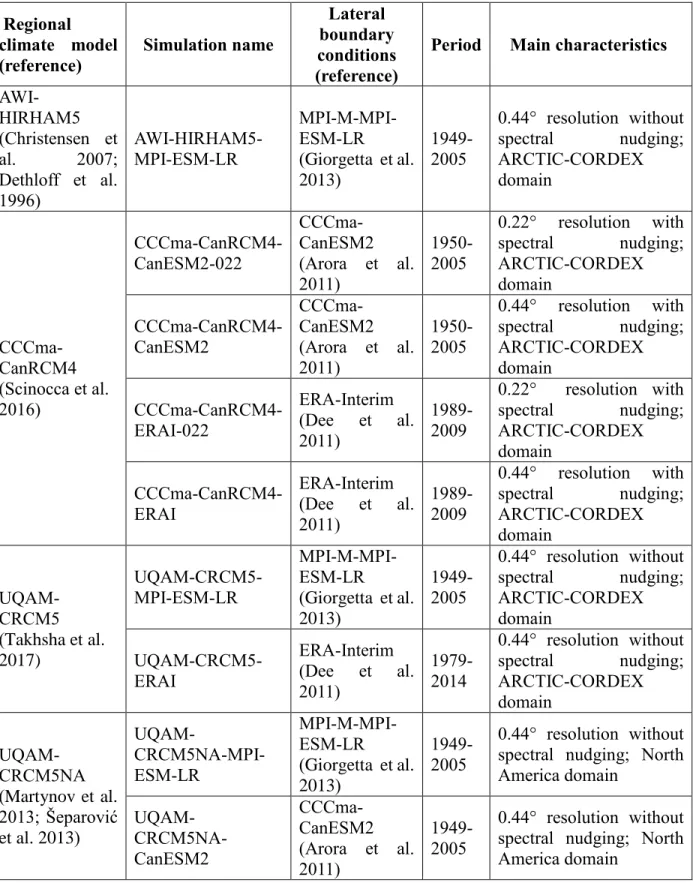
This study used four RCMs (AWI-HIRHAM5, CCCma-CanRCM4, SMHI-RCA4 and UQAM-115
CRCM5) that are part of the ARCTIC-CORDEX experiment ( http://www.climate-116
cryosphere.org/activities/targeted/polar-cordex/arctic). Table 1 provides information on the RCM 117
simulations, their characteristics and relevant references for each model with the ARCTIC-118
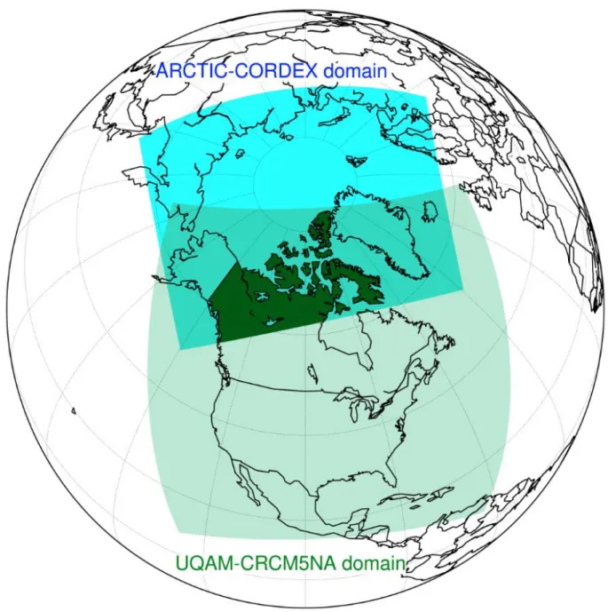
CORDEX domain shown in Figure 1. The simulations are driven by CMIP5 GCMs over a 119
historical period, mainly from 1951 to 2005 and by ERAI over a more recent period, mainly from 120
1989 to 2008. Some models used spectral nudging while others did not. For SMHI-RCA4 both 121
configurations, with (identified as SMHI-RCA4SN) and without (identified as SMHI-RCA4) 122
spectral nudging, were considered. The CCCma-CanRCM4 simulations were provided on a rotated 123
grid at two horizontal grid spacings, 0.44° and 0.22°, while the other model simulations were only 124
available at the 0.44° (about 50 km) horizontal resolution. The CORDEX-ARCTIC ensemble was 125
supplemented with three 0.44° horizontal-resolution simulations carried out with the UQAM-126
CRCM5 model over a North America domain, which completely covers Canada (Fig. 1), unlike 127
the North America CORDEX simulations. These three simulations are identified as UQAM-128
CRCM5NA (NA for North America) to differentiate them from the runs carried out over the 129
CORDEX-ARCTIC domain. The CCCma-CanRCM4 simulations at 0.22° are identified as 130
CCCma-CanRCM4-022. In total this provided twelve GCM-driven simulations and six ERAI-131
driven simulations for analysis. The analysis was carried out over the Canadian Arctic land areas 132
contained in the ARCTIC-CORDEX domain represented in Fig. 1 by the dark green shading. 133
2.2 Atmospheric reanalyses and gridded surface observations 134
The second goal of the study was to evaluate how well reanalyses and gridded surface 135
observation datasets capture the observed local climate from station records to determine if they 136
can be used in model evaluation to complement the observed station data. Six datasets were 137
6 considered comprising four recent reanalyses (CFSR, ERAI, JRA55, MERRA), and one product 138
that corrects the NCEP-R1 reanalysis with observed temperature, precipitation and radiation 139
(GMFD). Dataset descriptions and relevant references are presented in Table 2. For the Arctic 140
region and the period used in this study, the temperature observations used by GMFD are mainly 141
from the CRU TS3.0 gridded (0.5° x 0.5°) dataset, precipitation is corrected for undercatch and is 142
downscaled based on relationships developed with the Global Precipitation Climatology Project 143
daily product. Corrections were also made to high-latitude wintertime rain day statistics to remove 144
a spurious wavelike pattern (Sheffield et al. 2006). The gridded surface observation dataset 145
(NRCan) was included in the study to investigate the potential impacts of interpolating data from 146
sparse surface observations on climate indices. The NRCan dataset provides daily precipitation 147
and temperature from Environment and climate change Canada stations gridded on a horizontal 148
grid of ~ 10 km using the thin plate smoothing spline implemented in the ANUSPLIN climate 149
modelling software (Hutchinson et al. 2009). A two-stage approach was applied for interpolating 150
daily precipitation by estimating the spatial domain where precipitation occurred prior to carrying 151
out the interpolation of observed precipitation amounts. Trace precipitation amounts for solid 152
precipitation were assigned values from 0.03 to 0.07 mm that varied inversely with latitude 153
following Mekis and Vincent (2011). 154
CFSR, MERRA and ERA-Interim monthly mean temperature and precipitation data were 155
previously evaluated over the Canadian Arctic by Rapaić et al. (2015) and over the entire Arctic 156
by Lindsay et al. (2013). Both papers indicate that MERRA and ERA-Interim have relatively small 157
warm and wet biases compared to other reanalyses, while CFSR was found to have particularly 158
large positive precipitation biases. 159
2.3 Surface observations: 160
As previously mentioned, the number of stations with long-term daily temperature and 161
precipitation records across the Canadian Arctic remains small. The interpolation errors in gridded 162
products based on sparse station networks can be high, especially for extremes and climate indices 163
(e.g. Hofstra et al. 2010; Contractor et al. 2015; Way et al. 2016). As a consequence, climate model 164
evaluations over such regions are often carried out using station observations or reanalyses (e.g. 165
Lindsay et al. 2014; Glisan and Gutowski 2014a and 2014b; Matthes et al. 2010; Matthes et al. 166
2015; Wilson et al. 2012). In this study, we use surface observations of mean, minimum and 167
7 maximum daily temperature (Tmean, Tmin and Tmax, respectively) and daily precipitation (Pr) 168
from the climate stations included in the National Climate Data and Information Archive at 169
Environment and Climate Change Canada (http://ccds-dscc.ec.gc.ca/index.php?page=download-170
obs) that have at least 15 valid years in the 1980-2004 validation period of GCM-driven RCM 171
simulations. Where stations were adjusted and corrected for known systematic errors, we used the 172
corrected station data from the Adjusted Historical Canadian Climate Data set (AHCCD; Vincent 173
et al. 2002, Vincent et al. 2012, Mekis and Vincent 2011). The AHCCD takes account of 174
systematic errors from changes in observing programs, instrumentation and station moves (the 175
latter for temperature data only), and also includes station joining to produce longer records. 176
Precipitation records in the AHCCD have undergone rigorous quality control and adjustments to 177
account for known measurement issues such as wind-induced undercatch, evaporation loss, and 178
adjustments for trace observations that are particularly important for the frozen and light 179
precipitation regimes that dominate the Canadian Arctic (Devine and Mekis 2008; Mekis 2005). 180
The water equivalent of the snowfall was adjusted based on climatological estimates of fresh 181
snowfall density obtained from stations where both Nipher gauge (solid precipitation) and snowfall 182
were measured (Mekis and Brown, 2010). Trace snowfall amounts were assigned values between 183
0.03-0.07 mm that varied inversely with latitude. 184
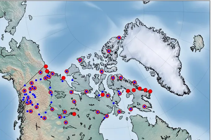
This resulted in a total of 47 stations for the air temperature indices evaluation and 78 stations 185
for the precipitation indices evaluation, with the spatial distribution shown in Figure 2. For the 186
1989-2005 period used in the comparison of the GCM-driven and ERAI-driven simulations, these 187
conditions were relaxed to at least 10 valid years, which led to similar numbers of stations: 48 188
stations for temperature and 79 for precipitation. Details concerning the station selection criteria 189
for climate indices computation are provided in Section 3. 190
It is important to note that none of the reanalyses considered in this study assimilated surface 191
precipitation data and that CFSR, MERRA, and JRA55 do not assimilate surface air temperature. 192
Surface air temperatures from Canadian synoptic stations are assimilated in ERA-Interim through 193
an analysis based on the Optimal Interpolation procedure, while GMFD is using a post-processing 194
procedure based on the CRU TS3.0 gridded (0.5° x 0.5°) monthly dataset that contains Canadian 195
climate station data. Consequently, surface air temperature fields from ERA-Interim and GMFD 196
are not completely independent from the temperature field of the AHCCD dataset. 197
8 3. Methodology
198
The five reanalyses and the GCM- and ERAI-driven simulations cover different periods of 199
time. In the first part of this study, the reanalyses and GCM-driven simulations were evaluated 200
over a common reference period of 25 years (1980-2004) while, in the second part, GCM- and 201
ERAI-driven RCM simulations were evaluated over a common period of 17 years (1989-2005). 202
3.1 Climate indices computation 203
The Expert Team on Climate Change Detection and Indices (ETCCDI; Klein Tank et al. 2009) 204
proposed a large number of climate indices that characterize many aspects (not only extremes) of 205
daily temperature and precipitation distributions relevant for climate change detection and climate-206
related applications. Also the ArcticNet Network of Centres of Excellence of Canada has identified 207
several climate indices relevant for climate change impacts and adaptation studies in the Canadian 208
Arctic (Allard and Lemay 2012; Stern and Gaden 2015). The reported indices were selected based 209
on regional interests after due consultation of local representative involved in natural, health, 210
social, and Inuit organizations, northern communities and federal and provincial agencies. In our 211
study, fifteen daily temperature and ten daily precipitation climate indices associated with key 212
characteristics of the precipitation and temperature regimes of the Arctic region were selected from 213
those proposed by the ETCCDI and Arctic impacts-relevant indices provided by the Canadian 214
ArcticNet program (Table 3). 215
It was however, necessary to adapt the nomenclature of certain ETCCDI indices to take account 216
of Arctic conditions. A large portion of the analysis domain is located north of the Arctic Circle 217
(66°32'N) that experiences polar days and nights with a less distinct diurnal cycle. Because the 218
notion of night and day is different for the Arctic, the term “day” will be used to denote a calendar 219
day of 24 hours and not the period of sunlight, and the indices were named as in Table 3. The 220
annual “cool” temperature indices were related only to the variable “daily minimum temperature” 221
(TNn, TN10 and TN10p), while the annual “warm” temperature indices are related only to the 222
variable “daily maximum temperature” (TXx, TX90 and TX90p). 223
While total precipitation is generally low over much of the Canadian Arctic (the Arctic islands 224
being known as Arctic desert (Serreze and Barry 2005, Stern and Gaden 2015), increases in 225
extreme precipitation events and precipitation intensity have been observed over the Arctic (Cohen 226
et al. 2014, Ye et al. 2015, Wan et al. 2015) and further increases are expected in response to 227
9 warming and increasing atmospheric humidity from reductions in sea ice extent. Therefore part 228
of this paper is devoted to evaluating model skill in simulating the upper-tail of daily-precipitation 229
annual distributions (Rx1day, Rx5day, R95ptot and R99ptot) and one related to the number of wet 230
days (R1mm), with a wet day defined as a day with precipitation ≥ 1 mm/day as these may be 231
impacted by climate change. 232
Some annual indices were defined using thresholds associated to percentiles computed over a 233
reference period (e.g. TN10p, TX90p, R95ptot and R99ptot). The 1980-2004 period (25 years) 234
was used as reference period for stations, reanalysis and GCM-driven simulations. For the 235
comparison of GCM- and ERAI-driven simulations, these indices were estimated over the 17-year 236
period 1989-2005. 237
In addition to these ETCCDI indices, annual, summer (June, July and August) and winter 238
(December, January and February) mean daily precipitation, annual, summer and winter mean 239
daily temperatures, heating degree days (HDD), growing degree days (GDD), freezing degree days 240
(FDD), thawing degree days (TDD) and number of winter thaw events (Nthaw) were also 241
estimated. 242
The GDD index is important in the Arctic for studies related to the growth, timing of vegetation 243
green-up onset, insect development and migration (Herms 2004, Sridhar and Reddy 2013), which 244
are key variables for caribou population, a major resource for local communities (Moerschel and 245
Klein 1997, Stern and Gaden 2015). The TDD index is closely related to snow melt processes, the 246
depth of the permafrost active layer and the initialisation of snowpack ablation (Stern and Gaden 247
2015), while the FDD index is related to ice growth and the depth of ground frost penetration 248
(Stern and Gaden 2015) which are relevant for transportation (e.g. ice roads) and infrastructure. 249
The Nthaw index is related to the production of ice layers within or under the snowpack that may 250
limit caribou access to forage. 251
The climate indices were computed at each point of the original grid for each 252
simulation/reanalysis as suggested in Diaconescu et al. (2015). For stations, annual indices were 253
computed only for years with less than 20% missing values, defined as a valid year. 254
3.2 Evaluation metrics 255
10 Evaluation of models and reanalyses is usually carried out by comparing area-averaged 256
statistics (e.g. mean values, variances) or by comparing the distributions of values of co-located 257
pairs. The latter approach is difficult in our situation due to the limited number of years of data. 258
Hansen et al. (2012) and Hansen and Sato (2016) proposed to pool data from different stations 259
within a region into a single sample in order to increase the sample size. This approach is 260
reasonable as long as the value of interest over that region can be considered homogeneous, i.e. 261
that the local values can be described by a unique distribution. A similar method was adopted by 262
Alexander et al. (2006) in the analysis of global climate annual indices from a subset of 200 263
temperature and 350 precipitation stations across the globe. Donat and Alexander (2012), Hansen 264
et al. (2012), and Hansen and Sato (2016) used probability density distributions of temperature 265
anomalies over specific regions rather than absolute-value distributions because the anomalies 266
have a higher spatial correlation, while absolute mean temperatures can vary over short spatial 267
scales (Hawkins and Sutton 2016). Consequently, even a few stations can capture the temporal 268
characteristics of anomalies over a large region. We therefore chose to use this approach and 269
pooled the anomalies to compare the distributions. 270
Consequently, each local climate index value 𝑌(𝑙𝑜𝑛, 𝑙𝑎𝑡, 𝑡) was decomposed into the local 271
climatological mean, 𝑌(𝑙𝑜𝑛, 𝑙𝑎𝑡), and the local anomalies 𝑌′(𝑙𝑜𝑛, 𝑙𝑎𝑡, 𝑡):
272
𝑌(𝑙𝑜𝑛, 𝑙𝑎𝑡, 𝑡) = 𝑌(𝑙𝑜𝑛, 𝑙𝑎𝑡) + 𝑌′(𝑙𝑜𝑛, 𝑙𝑎𝑡, 𝑡) Eq. 1
273
The local climatological mean corresponds to the mean value over the reference period at a specific 274
site. The local anomalies were obtained by subtracting the local climatological mean from the local 275
annual index value. The spatial distribution of the climatological mean and the distribution of 276
anomalies were then estimated. Model and reanalysis skill in simulating the spatial patterns of the 277
climatological mean were evaluated (Section 4.1.1) as well as the distribution of anomalies 278
(Section 4.1.2). 279
For the spatial pattern evaluation, the Mean Squared Skill Score (MSSS; see e.g., Murphy 280
1988; Murphy and Epstein 1989) was used. It compares the Mean Square Error (MSE) of a forecast 281
(a given RCM simulation or reanalysis) with respect to the observations (f;o) to the MSE of a 282
selected reference dataset with respect to the observations (r,o): 283
𝑀𝑆𝑆𝑆 = 1 −𝑀𝑆𝐸(𝑓,𝑜)𝑀𝑆𝐸(𝑟,𝑜) Eq. 2
11 A positive value indicates that the forecast has a greater skill than the reference, with MSSS = 285
1 indicating a perfect forecast skill and MSSS ~ 0 similar forecast and reference skills. For instance 286
if the forecast values more closely match observed values than the reference dataset then MSE(f,o) 287
< MSE(r,o) and 0 < MSSS ≤ 1 (otherwise MSSS ≤ 0). 288
In this study, two versions of the MSSS were used to evaluate reanalysis and RCM skill in 289
simulating the spatial patterns of climatological mean of indices over the Canadian Arctic: 290
1) MSSS with reference to the variance of observations also known as the Reduction of 291
Variance (RV) metric. For a given climate index, this score compared the MSE between 292
the mean for a given dataset (RCM simulation or reanalysis) to the spatial variance of the 293
climatological mean of observations over the region (𝑠𝑜2 = 1
𝑁∑ (𝑂̅𝑖 − 〈𝑂̅〉)2 𝑁 𝑖=1 ): 294 𝑅𝑉𝑘 = 1 −𝑀𝑆𝐸(𝑘,𝑂)𝑠 𝑜2 = 1 − ∑𝑁𝑖=1(𝑌𝑘𝑖−𝑂𝑖)2 ∑𝑁𝑖=1(𝑂𝑖−〈𝑂〉)2 Eq. 3 295
with 𝑌𝑘𝑖 representing the climatological mean of dataset k (a RCM simulation or a 296
reanalysis) at the grid point closest to station i, 𝑂𝑖 the recorded observational climatological 297
mean at station i, 〈𝑂〉 the spatial mean over the analysis region (see Fig. 1) of observational 298
climatological mean at stations and N the number of stations in the region. The 299
model/reanalyses MSE is computed with respect to observations (𝑀𝑆𝐸(𝑘, 𝑂) = 300
1
𝑁∑ (𝑌̅𝑘𝑖 − 𝑂̅𝑖) 2 𝑁
𝑖=1 ). A value of RVk > 0 means that dataset k has a smaller MSE value than 301
the spatial variance in observations. 302
2) Another version of the MSSS compares the MSE of the index climatological mean of a 303
given dataset to the MSE value averaged over all reanalyses: 304
𝑀𝑆𝑆𝑆𝑘= 1 −1𝑀𝑆𝐸(𝑘,𝑂) 5∑5𝑟=1𝑀𝑆𝐸𝑟
Eq. 4 305
with MSE(k,O) representing the MSE of a given dataset k (either model simulation or 306
reanalysis) and MSEr representing the MSE of reanalysis r. The denominator sum in 307
Equation 4 is over all five reanalysis datasets. This version is particularly useful because it 308
compares individual RCM performance to mean reanalysis performance (a value of MSSSk
309
> 0 means that dataset k outperformed the mean reanalysis performance). It also provides 310
12 information regarding the use of reanalyses as reference datasets for model evaluation in 311
the Arctic region. 312
Evaluation of anomaly distributions, for each given index, was performed by pooling all annual 313
anomalies at stations and corresponding grid-point values over the Canadian Arctic Region. 314
Corresponding empirical distributions were then constructed. 315
The ability of reanalyses and models in simulating station anomaly distributions was assessed 316
with the Kuiper goodness-of-fit metric (Kuiper 1960) and the Perkins metric (Perkins et al. 2007). 317
The two metrics were considered to check whether they provided consistent conclusions. Both 318
metrics have the advantage of not depending on the shape of the underlying distribution and they 319
can be applied to any variable. 320
The Kuiper metric, inspired from the Kolmogorov-Smirnov test, is one of the most commonly 321
used methods to compare distributions from two samples (Smirnov 1939; Stephens 1970). It 322
measures the distance between the two empirical cumulative distributions and is defined as the 323
sum of the absolute values of the maximum positive and negative distances between the two 324
empirical cumulative distributions: 325
𝐷𝐾 = max−∞<𝑥<∞[𝐸𝐶𝐷𝐹𝑘(𝑥) − 𝐸𝐶𝐷𝐹𝑜(𝑥)] + max−∞<𝑥<∞[𝐸𝐶𝐷𝐹𝑜(𝑥) − 𝐸𝐶𝐷𝐹𝑘(𝑥)] Eq. 5
326
with ECDFk and ECDFo representing the empirical cumulative distributions of dataset k and of 327
recorded datasets respectively. DK values range between zero and one, with zero indicating a 328
perfect overlap of the two distributions while a value of one corresponds to no overlapping 329
distributions. 330
The Perkins metric is defined as the overlap between the two empirical probability density 331
functions (EPDF) and has been used in evaluating temperature and precipitation series simulated 332
by GCMs (Perkins et al. 2007; Maxino et al. 2008; Pitman and Perkins 2009; Perkins 2009; Perkins 333
et al. 2012) as well as RCMs (Kjellstrom et al. 2010; Kabela and Carbone 2015; Boberg et al. 334
2010). Here we extend its use by evaluating climate index anomaly distributions. Normalised 335
histograms of indices from reanalyses and simulations were compared with corresponding index 336
histograms from recorded datasets. The size of the bin used for each index is presented in Table 3. 337
The bins were selected to cover the whole range of values of both datasets. The common area 338
between the two distributions was computed as: 339
13 𝑃𝑆𝑆𝑘 = ∑𝑛𝑥=1𝑚𝑖𝑛𝑖𝑚𝑢𝑚(𝐸𝑃𝐷𝐹𝑘(𝑥), 𝐸𝑃𝐷𝐹𝑂(𝑥)) Eq. 6
340
where n is the number of bins used to calculate the normalised histograms, EPDFk (x) is the 341
frequency in bin x for the dataset k, EPDFO(x) is the corresponding frequency for the recorded 342
dataset in bin x. PSS values range from zero to one, a zero value corresponding to no overlap 343
between the two histograms and one to identical histograms. To ease the comparison with Kuiper 344
metric, the (1-PSS) metric will be used in the following. 345
In summary, the RV and MSSS metrics were used to compare the performance of the 346
climatological mean, while the Kuiper and Perkins metrics were used to compare the performance 347
of the distribution of annual anomalies (i.e. the annual departures from the climatological mean). 348
349
4. Evaluation of GCM-driven RCM and reanalyses indices 350
4.1 Climatological means 351
Index climatological means are presented first at stations over the Canadian Arctic (Section 352
4.1.1). Next the skill of models and reanalyses at reproducing the observed values are evaluated 353
using the RV metric, biases and the MSSS metric (Sections 4.1.2 to 4.1.4). 354
4.1.1 Observed climatological means 355
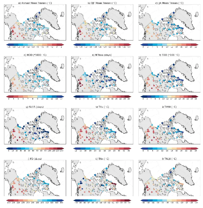
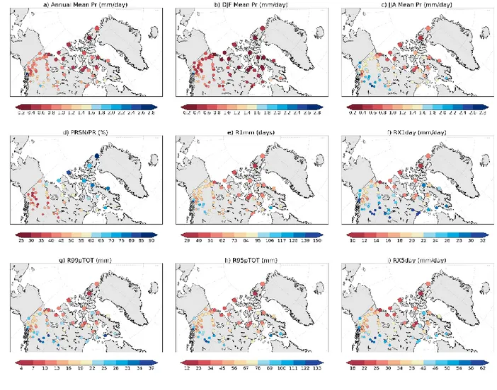
The spatial coherence of the observed climate indices at stations was first examined visually 356
(see Figs. 3 and Fig. 4 for the climatological means of selected indices). Most of the temperature 357
indices showed important spatial gradients over the Arctic, consistent with the radiative forcing. 358
The only exception was the annual coldest temperature (TNn; Figure 3k), which is influenced by 359
local scale factors such as proximity to open water and topography that influence inversion layer 360
formation (Rapaić et al. 2015). 361
For precipitation indices, the entire domain is characterised by relatively small amounts of 362
precipitation, with most stations having mean annual precipitation rates of less than 1.0 mm/day 363
(Figure 4a). More precipitation arrives in the summer period than winter (Figs. 4b and c) because 364
warmer temperature in summer and the presence of ice-free water (lakes and Arctic Ocean) 365
increase atmospheric moisture. The fraction of total precipitation falling in solid form is varying 366
from 30% to 90% over the region (Fig. 4d). Solid precipitation (PRSN/PR between 60% and 367
100%) dominates in the north where the mean annual precipitation is very low (less than 1 368
mm/day), while liquid precipitation is more important over the southern regions (PRSN/PR 369
between 40% and 20%) where mean annual precipitation has values between 1.2 mm/day and 2.8 370
14 mm/day. Analysis of daily-precipitation distributions shows that higher intensity daily 371
precipitation can occur especially in the southern part of the domain and in some coastal regions 372
with open water during the summer. Also, in summer, extratropical cyclones can penetrate further 373
north and can reach the Hudson Bay, in winter such trajectories are unlikely (Reitan 1974). 374
Consequently, precipitation is generally less extreme over the northern regions of the study area 375
(RX1day/RX5day less than 20/30 mm/day; R99pTOT less than 16 mm and R95pTOT less than 376
45 mm) and more extreme over southwestern regions and south of Baffin Island (RX5day between 377
30 mm/day and 70 mm/day and R99pTOT with values between 20 mm and 40 mm). 378
4.1.2 RV metric 379
The performance of the models and reanalysis in simulating the spatial patterns of the 380
climatological means of the precipitation and temperature indices was first evaluated using the RV 381
metric (Eq. 3), which was computed using the station records as a reference as described in Section 382
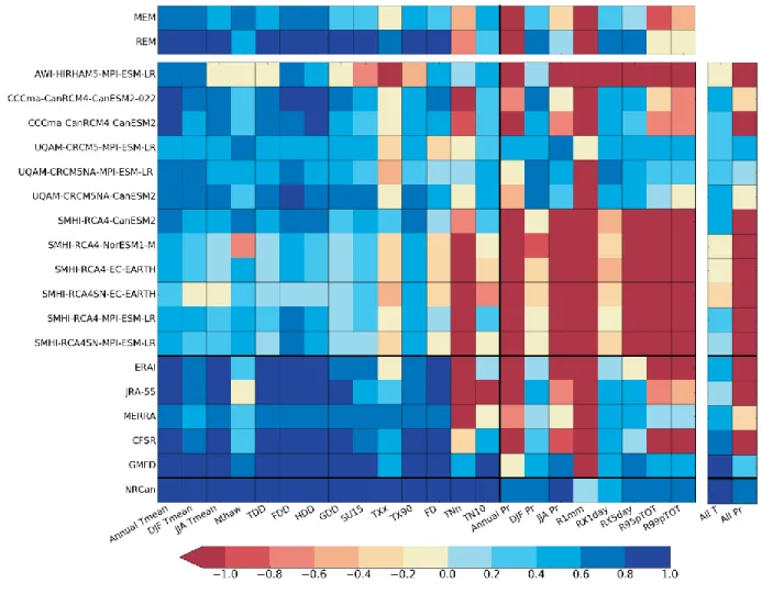
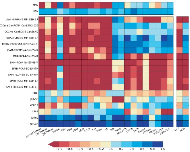
2.3 and presented in Section 4.1.1. Heat maps in Figure 5 summarize the estimated RV values with 383
columns representing the indices, and rows the datasets. The last two columns denoted “All T” 384
and “All Pr” present the average performance of each data set in simulating all temperature indices 385
(All T) and all precipitation indices (All Pr), and corresponds to the mean RV value over all 386
temperature or precipitation indices of the corresponding dataset. The top two rows of Figure 5 387
present the RV of the ensemble mean of reanalyses (identified as REM and corresponding to the 388
RV values of the corresponding index averaged over all five reanalyses) and of the model ensemble 389
mean (identified as MEM and corresponding to the RV values of the corresponding index averaged 390
over all simulations). In the following, for ease of interpretation, ‘good skill’ (or ‘good 391
performance’) will be associated with positive RV values (blue boxes in Figure 5), for which the 392
squared differences between model/reanalysis and station indices were smaller than the recorded 393
spatial variance among stations, while ‘poor skill’ (or ‘poor performance’) will be associated with 394
negative RV values (red boxes in Figure 5), for which the MSE of a model/reanalysis were greater 395
than the spatial variance among stations. 396
Figure 5 shows that the overall model and reanalysis performance was better for the 397
temperature indices (first fourteen columns) than for the precipitation indices (last eight columns). 398
Ten of the temperature indices (Annual Tmean, DJF Tmean, JJA Tmean, Nthaw, TDD, FDD, 399
HDD, GDD, SU15 and TX90) were well simulated by all reanalyses and almost all RCM 400
simulations. The reanalyses demonstrated a good ability at simulating the FD and TXx indices 401
15 (only ERAI has a negative RV for TXx), while many RCM simulations were less effective for 402
these two indices. The TNn index was poorly reproduced by most of the reanalysis and RCM 403
simulations. The reanalyses’ performance was better than the RCMs for eleven of the fourteen 404
temperature indices, as also indicated by the REM and MEM performances. For Nthaw and TN10, 405
MEM was better than REM, while for TNn both MEM and REM had negative RV values. 406
The climatological means of DJF Pr (16th column of Fig 5), RX1day (19th column of Fig 5) 407
and RX5day (20th column of Fig 5) indices were well reproduced by most reanalysis and by the
408
CCCma-CanRCM4 and UQAM-CRCM5 simulations. The ability to reproduce these indices was 409
also reflected by the positive RV of REM and MEM. Only two reanalysis (GMFD and MERRA) 410
and the UQAM-CRCM5 simulations were capable of reproducing the climatological mean of 411
R95pTOT (21th column of Fig 5) and R99pTOT (22th column of Fig 5). Also, all reanalysis and 412
most RCM simulations showed poor performance for Annual Pr (15th column of Fig 5), JJA Pr 413
(17th column of Fig 5) and R1mm (18th column of Fig 5) indices. Therefore, the reanalyses and 414
some models were able to effectively reproduce the annual extremes of daily precipitation (R1days 415
and RX5days) but show poor performance for the annual and summer mean of daily precipitation 416
(Annual Pr and JJA Pr) and the annual number of wet days (R1mm) indicating a frequency bias in 417
the occurrence of precipitation. While RCMs have similar skill in simulating the DJF Tmean and 418
JJA Tmean, reanalyses show better skill for the summer mean temperature. Almost all RCMs and 419
reanalyses have better scores in simulating DJF Pr than JJA Pr. 420
Figure 5 also compares the performances of different configurations of the same RCM. For the 421
SMHI-RCA model, configurations with (SMHI-RCASN) and without (SMHI-RCA) spectral 422
nudging were evaluated and show that the configuration without spectral nudging had superior 423
skill for some temperature indices, while performances were similar for precipitation indices. 424
For the CCCma-CanRCM4 model, simulations with two spatial resolutions were compared. 425
Figure 5 shows that the model configuration at 0.22° resolution (CCCma-CanRCM4-CanESM2-426
022) had better performance than the 0.44° configuration (CCCma-CanRCM4-CanESM2) for DJF 427
Tmean, FDD, GDD, SU15, FD, Annual Pr, DJF Pr, RX5day and R95pTOT indices. Conversely, 428
the other indices had similar performances. 429
4.1.3 Biases 430
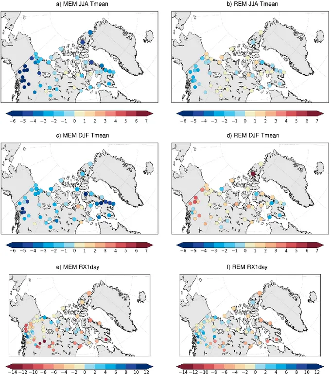
To examine the potential influence of geography in model performance, the spatial patterns of 431
the differences in climatological mean values between MEM/REM and observations for the DJF 432
16 Tmean, JJA Tmean and RX1day indices are presented in Figure 6. These patterns are 433
representative of most RCMs and reanalysis and most indices: DJF Tmean for cold and winter 434
temperature indices (Nthaw, DJF Tmean, TN10, TNn), JJA Tmean for warm temperature and 435
degree-day indices, and RX1day for precipitation indices. The analysis of the spatial distribution 436
of the RCM/reanalysis - observations differences for all temperature indices showed different 437
patterns for cold and winter-time indices and all other temperature indices. Most reanalyses and 438
especially RCMs present a larger bias over the Yukon high-topography region for the warm indices 439
and the annual daily degree indices (Fig. 6a and 6b), while the cold indices don’t display any 440
particular pattern (Fig. 6c and 6d). The larger negative errors observed over the mountain region 441
in indices incorporating the summer temperatures (Fig. 6a and 6b) can be due to the difference in 442
topographic elevation in RCMs/reanalyses and stations, stations being usually located in valleys. 443
Consequently, RCMs/reanalysis temperatures are usually colder than temperatures recorded at 444
stations since mean grid-point elevations of RCMs/reanalysis are typically higher than station 445
elevations. 446
These results suggest that some bias correction based on the temperature climatological lapse 447
rate for this region should be applied to correct station temperatures. However, the difference 448
between station altitude and corresponding RCM/reanalysis mean grid-point elevation doesn’t 449
seem to affect cold and winter indices (Figs. 6c,d), for which no structured spatial distribution of 450
differences was observed. In Fig. 6, mean temperature from reanalyses are warmer than observed 451
ones (Fig. 6d) while models simulate colder mean temperatures over most part of the Arctic (Fig. 452
6c). This difference in spatial pattern of the bias between warm and cold temperature indices can 453
be explained by the high frequency of surface and upper tropospheric temperature inversions 454
during the cold period (December to March) caused by the radiative surface cooling or by the 455
warmer air advection over the arctic cold air masses (Lovatt 2009, Serreze and Barry 2005, 456
Przybylak 2016). Important «semi-permanent» inversions are present especially in the deep 457
valleys of the Yukon and the Alaska mountainous regions (Lovatt 2009, Przybylak 2016). 458
Consequently, local processes have a high impact on cold indices and a bias correction based on 459
the climatological lapse rate would not be appropriate to correct cold daily temperature series. 460
Statistical methods or more complex physical methods that incorporate local processes 461
conditioning the seasonal evolution of the local lapse rate would be needed to adequately correct 462
daily minimum, maximum and mean temperature indices over this specific region. Precipitation 463
17 indices do not present a particular pattern in the bias (see for example RX1day bias in Fig. 6e and 464
Fig. 6d) with the exception of higher bias values for more southerly points and those close to the 465
Pacific Coast (especially for Annual Pr and R1mm indices – not shown) where mean and extreme 466
precipitation amounts are larger (see Fig. 4). 467
In summary, for temperature indices, reanalyses and RCMs generally performed well in 468
simulating the climatological means of mean-daily and maximum-daily temperature indices over 469
most Canadian Arctic. The bias is generally larger over the Yukon region in indices based on 470
summer temperatures. RCMs and reanalyses were less effective at simulating the TNn index. 471
Regarding precipitation indices, most reanalyses and some RCMs were able to reproduce 472
climatological means of DJF Pr, RX1day and RX5day indices effectively, but were less effective 473
in simulating the Annual Pr and the R1mm indices. 474
Violin plots (Hintze and Nelson 1998; computed using the Seaborn Python package: 475
https://stanford.edu/~mwaskom/software/seaborn/index.html) were used in Fig. 7 to examine the 476
climatological mean biases of TNn, R1mm (that were poorly represented by reanalyses and 477
models) and RX1day (that was well simulated by most reanalyses and RCMs). Violin plots show 478
the density of the distribution of biases over the Canadian Arctic based on a kernel smoother. The 479
more “squashed” the violin and the closer the median (white dot) is to zero, the closer the values 480
are to the observations. The first violin of each graph corresponds to the NRCan dataset and shows 481
the biases between grid-point index values and corresponding values at the closest stations. The 482
next three violins, in green, capture the range of results from the reanalyses i.e. the reanalysis with 483
the lowest RV metric (left), the reanalysis ensemble mean (REM) (middle), and the reanalysis 484
with the largest RV value (right). The range in RCM simulations is similarly represented by the 485
three magenta violins. 486
For the TNn index, the interpolation process in NRCan smoothed the minimum daily 487
temperature values resulting in an overall small positive bias on most of the grid points close to 488
stations, with the median bias equal to 0.63° C. All reanalyses displayed an overall warm bias in 489
agreement with previous studies (e.g. Rapaić et al. 2015) with a median bias of +3.4°C for REM. 490
Contrary to reanalyses, RCMs had a cold bias in TNn with MEM bias of approximately -2.8°C. A 491
warm bias in reanalyses and a cold bias in simulations was also observed for the 10th percentile of 492
minimum daily temperatures (TN10 index), but with smaller amplitude than for the TNn index 493
(not shown). The poor performance of RCMs and reanalyses in simulating the cold extremes, is 494
18 attributed in part to a lack of local-scale information related to inversion layer development. The 495
representation of atmospheric humidity profiles and clouds in models/reanalyses would also play 496
roles in radiative cooling. 497
Four of the five reanalyses and all RCM simulations displayed positive R1mm biases, and 498
therefore a larger number of wet days than recorded at the stations, with maximum biases in the 499
southwestern region of the domain characterised by high topography (see Figure 2). Small negative 500
biases were observed for the northern regions. An exception was the GMFD product with a smaller 501
number of wet days than observations over a large part of the domain (median bias of -20 days per 502
year) and the UQAM-CRCM5-MPI-ESM-LR simulation, which had the smallest model-and-503
reanalysis median bias (approximately 7 days per year) similar to the NRCan median bias 504
(approximately 6 days per year). 505
The interpolation procedure has an important impact on the estimated NRCan RX1day index 506
(see Figure 7c; Hutchinson et al. 2009). The interpolation process introduces a smoothing of daily 507
precipitation that results in a negative bias for RX1day (underestimation of RX1day values 508
estimated from recorded series) for almost all NRCan grid points next to stations (only two stations 509
in the north had positive biases and these stations were probably not integrated with the NRCan 510
product). NRCan biases ranged from -9.9 mm/days to +1.0 mm/day with a median bias of -4.0 511
mm/day, a value larger than the REM (-0.9 mm/day) and MEM median biases (-1.9 mm/day). 512
REM good performance was also illustrated by the RV metric presented in Figure 5, REM has a 513
greater RV value than NRCan for this index. The best reanalysis performance for this index was 514
obtained for JRA55 with a median bias of -1.6 mm/day. This value was larger than the REM 515
median bias, the good REM performance being in part due to bias compensation in the average 516
process across the five reanalyses (positive and negative biases compensating each other). The best 517
performance for RX1day index was obtained by UQAM-CRCM5NA-MPI-ESM-LR simulation 518
that has a median bias of -0.79 mm/day, which was better than all five reanalyses and the NRCan 519
dataset. Overall, the median biases for REM and MEM were similar and close to the best 520
RCM/reanalyses value. 521
4.1.4 MSSS metric 522
The skillfulness of the RCMs and reanalyses simulations were also compared by using the 523
mean MSE of reanalyses as a reference dataset in the MSSS metric (Eq. 4). The corresponding 524
heat maps are plotted in Figure 8 where, as in Figure 5, each row corresponds to a dataset and each 525
19 column to an index. The top two lines compare REM and MEM MSE to the mean MSE of the five 526
reanalyses, while the last two columns show the average value of the MSSS metrics for all 527
temperatures (‘All T’) and precipitation (‘All Pr’) indices for a given dataset. The positive MSSS 528
values, in blue, signify that the dataset outperformed the mean reanalysis performance. 529
The performances of the RCM simulations were below the mean performances of reanalyses 530
for all temperature indices (negative values for MSSS metric), except for the Nthaw and the cool 531
extreme indices TNn and TN10. For the mean-temperature and maximum-temperature indices (the 532
first 12 columns), all reanalyses demonstrated good performances (e.g. Figure 5), with GMFD 533
performance well above the mean reanalysis value (positive values for MSSS metric), CFSR 534
performance close to the mean reanalysis performance, and ERAI and MERRA performances 535
generally below the mean reanalysis value. 536
The overall excellent RV scores obtained for the reanalyses in Figure 5 suggest that these can 537
be used as reference dataset for RCM evaluation for mean and maximum temperature indices. 538
However, most reanalyses were not effective in simulating the TNn and TN10 indices. Moreover, 539
Figure 8 shows that most RCM simulations have errors smaller than or similar to the mean 540
reanalysis MSE for these indices. 541
For precipitation indices, the performances of the five reanalyses were similar, with GMFD 542
displaying an overall higher performance and with CFSR and ERAI having performances below 543
the average reanalysis value. The five simulations with CCCma-CanRCM4 and UQAM-CRCM5 544
had simulation performances superior to the reanalysis average. This suggests that reanalyses 545
should not be used as reference datasets for RCM evaluation for precipitation indices over the 546
Arctic. 547
As for the individual models, the performance of the MEM for the warm and mean temperature 548
extremes was below the average reanalysis performance, while for the cold extremes (TNn and 549
TN10), the Nthaw, the R1mm, R95pTOT and R99pTOT indices, it was above. Bias compensation 550
was more effective for REM presenting positive MSSS metric for all indices. Nevertheless, the 551
performances of UQAM-CRCM5 simulations were better than the REM performance for TNn, 552
Mean Pr, R1mm, R95pTOT and R99pTOT. 553
In summary, reanalyses outperformed RCM simulations for mean and warm daily temperature 554
indices and the best performances were obtained by GMFD and CFSR. This suggests that they 555
could be used as a reference in the RCM evaluation of daily temperature indices over the region. 556
20 However, for daily precipitation indices, the performances of reanalyses were lower and some 557
RCM simulations even outperformed all reanalyses. Caution is therefore recommended when 558
using reanalyses as reference datasets when evaluating RCM performance for daily precipitation 559
indices. 560
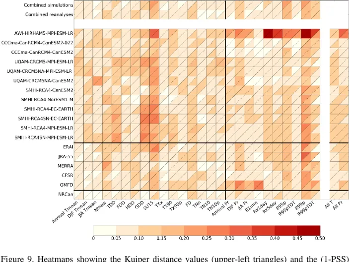
4.2 Anomaly distributions 561
Empirical distributions of anomalies from RCMs/reanalyses and surface observations were 562
compared to determine the skill of reanalyses and models in simulating the observed distributions. 563
Anomalies from all station records in the Canadian Arctic were pooled and ECDF and EPDF were 564
computed. The skills of reanalyses and models in simulating the observed distribution were 565
evaluated using Kuiper metric (D; Eq. 4) and Perkins skill scores (PSS; Eq. 5). The values obtained 566
for each climate index and for each dataset are plotted in Figure 9 using a diagram inspired by the 567
Performance Portrait diagram of Gleckler et al. (2008). 568
Figure 9 shows that the two metrics gave similar results in all cases (as a reminder a value of 569
zero corresponds to a perfect match of the two distributions). Reanalyses and RCMs were very 570
effective in simulating the anomalies’ distribution for most indices. Lower scores were obtained 571
by RCM simulations for GDD and SU15 indices and by RCM simulations and reanalyses for the 572
R99p index. Among the RCM simulations, the AWI-HIRHAM5-MPI-ESM-LR simulations 573
poorly reproduced anomaly distributions for R99p, Rx1day, Rx5day and SU15 indices, but had 574
excellent scores for DJF Tmean, NThaw, FDD, TXx, TX90p, TNn and R1mm indices. Figure 10 575
presents an example of the observations (in blue) and AWI-HIRHAM5-MPI-ESM-LR (in red) 576
Rx1day and TNn anomaly ECDFs and EPDFs. The figure highlights the similarity of simulated 577
and observed anomaly distributions for TNn index, characterised by a Kuiper distance of 0.05 and 578
(1-PSS) value of 0.06 (Figure 10b). For the RX1day index, the range of values of model anomalies 579
is smaller than that of observations, resulting into a smaller inter-annual variability. This is added 580
to an already poor performance for the climatological mean RX1day index (12th column in Figure
581
5). 582
When anomalies from all reanalyses or all simulations were pooled together (top two rows of 583
Figure 9), the resulting distributions resembled closely the recorded anomaly distributions (D < 584
0.1 and 1-PSS < 0.1) for a majority of the indices. Therefore, for reanalyses and RCM climate 585
indices over the Canadian Arctic, the main errors are related to bias in the mean index values, 586
while these datasets showed an overall good performance in simulating the anomaly distribution 587
21 over the region. These results suggest that, once the climatological mean of indices have been bias 588
corrected, some datasets, displaying good performance in reproducing the observed anomalies 589
over the Arctic region for a given index, can be used to assess its mean value over the Arctic, but 590
also its inter-annual variability. 591
592
5. Comparison of GCM-driven and ERAI-driven simulations 593
The skill of GCM-driven and ERAI-driven RCMs in simulating climate indices were compared 594
over a common period of 17 years (1989-2005). Most of the published RCM evaluation studies 595
have been conducted using RCM simulations driven by reanalyses, which presumably represents 596
the most realistic lateral boundary conditions. However, GCM-driven simulations are used to 597
develop climate projections and therefore the errors introduced by GCMs in these simulations 598
should be assessed. The comparison of errors in simulations driven by GCM with those driven by 599
reanalyses provides some information on the contributions of RCM structural bias and GCM bias 600
to the total errors. 601
Figure 11 presents the results of this comparison for six RCM configurations (CCma-602
CanRCM4 at 0.22° and at 0.44° resolution; UQAM-CRCM5 over Arctic and North-America 603
domains; SMHI-RCA with and without spectral nudging). Some RCM configurations where 604
driven only by one GCM (CCCma-CanRCM4; CCCma-CanRCM4_022; UQAM-CRCM5), while 605
some others were driven by two GCMs (UQAM-CRCM5NA, SMHI-RCASN) or four GCMs 606
(SMHI-RCA). Figure 11 compares, for each RCM configuration, the mean performance of the 607
GCM-driven simulations to that of the ERAI-driven simulation. The upper-left triangle in Figure 608
11 presents the mean performance for all simulations from a given RCM configuration driven by 609
GCMs, while the bottom-right triangle represents the performance of the same RCM configuration 610
driven by ERAI. The effectiveness of simulating the climatological mean (Figure 11a) was 611
measured using the Reduction of Variance as in the previous section, while the performance in 612
simulating the anomaly distribution (Figure 11b) was measured using Kuiper distance. 613
Figure 11 shows that differences in performance between GCM- and ERAI-driven simulations 614
were globally more pronounced for climatological means than for anomalies. In general, anomaly 615
distributions were very well reproduced by RCMs whether they were driven by GCMs or by ERAI 616
(in most cases D was smaller than 0.2). For a majority of indices, ERAI-driven simulations showed 617
better performance at simulating climatological means. SMHI-RCA4 and SMHI-RCA4SN had 618
22 negative RV metrics for TXx, FD and RX1day when driven by GCMs, but positive values when 619
driven by ERAI. These two RCM configurations poorly simulated TNn, Annual Pr, JJA Pr, R1mm, 620
R95pTOT and R99pTOT mean indices even when driven by ERAI. Note that ERAI did not 621
effectively simulate either of the latter indices (see Figure 5). 622
Negative RV values were also obtained for the CCCma-CanRCM4 simulations for TNn, 623
Annual Pr, JJA Pr and R1mm indices when driven by GCM or ERAI. Nevertheless, for R95pTOT 624
and R99pTOT indices, CCCma-CanRCM4_022, CCCma-CanRCM4, UQAM-CRCM5 and 625
UQAM-CRCM5NA, driven by GCMs and by ERAI, performed well, while ERAI did not (see 626
Figure 5 for RV of ERAI). Surprisingly, UQAM-CRCM5 and CCCma-CanRCM4 produced better 627
simulations when driven by a GCM than when driven by ERAI for these two precipitation indices. 628
This suggests that the simulated fields within the domain can be improved by these RCMs, 629
therefore adding value to the representation of ERAI for these indices. 630
The RCM-added value, with respect to ERAI, can also be assessed through the ratio of RCM 631
MSE and ERAI MSE as presented in Figure 12 for each mean climate index. CCCma-632
CanRCM4_022, CCCma-CanRCM4, UQAM-CRCM5, and UQAM-CRCM5NA produced 633
smaller MSE than ERAI for precipitation indices. The better representation of precipitation indices 634
by some RCMs is probably due to a better representation of the physics in these models as well as 635
to their higher spatial resolution. The comparison of the CCCma-CanRCM4_022 MSE with the 636
CCCma-CanRCM4 MSE also demonstrated that, for the Annual Pr, DJF Pr, JJA Pr, R1mm, 637
R95pTOT and R99pTOT indices, the higher resolution simulation provided a better simulation of 638
mean climate values. 639
Added value was also observed in GCM-driven and ERAI-driven UQAM-CRCM5 and 640
UQAM-CRCM5NA simulations of Nthaw, TNn and TN10 indices compared to ERAI. For SU15, 641
TXx and TX90, slightly better scores were obtained by some ERAI-driven RCMs than for ERAI. 642
For these indices, the RCM’s higher resolution may explain the slight improvement with respect 643
to ERAI. The fact that the corresponding GCM-driven simulations had lower performance than 644
ERAI for SU15, TXx and TX90 indices, is explained by the presence of larger errors in GCM 645
temperature fields than in the ERAI fields applied at the RCM lateral boundary conditions. 646
As expected, the overall performance in reproducing temperature indices depended on lateral 647
boundary datasets, ERAI-driven RCMs tending to have generally better scores than GCM-driven 648
RCM for these indices. 649
23 650
6. Summary and conclusions 651
The present study used climate station observations across the Canadian Arctic to evaluate five 652
daily precipitation and ten daily temperature indices simulated by (1) an RCM ensemble of twelve 653
GCM-driven simulations and six ERAI-driven simulations participating in the CORDEX 654
experiment, (2) five reanalyses products (GMFD, CFSR, MERRA, JRA-55 and ERAI) and (3) one 655
high-resolution gridded observational product (NRCan). The reanalysis and GCM-driven 656
simulations were first evaluated over a reference period of 25 years (1980-2004). Records from 47 657
stations for temperature and 78 stations for precipitation were used. Climatological means and 658
annual anomaly distributions were evaluated separately for each index and compared to 659
corresponding index values estimated from recorded datasets. The impact of lateral boundary 660
conditions was also analyzed by comparing the GCM-driven simulations to the corresponding 661
ERAI-driven simulations over a common period of 17 years (1989-2005). In this case, records 662
from 48 stations for temperature and 79 stations for precipitation were used. 663
The analysis of mean climate indices over the reference period showed that: 664
- The RCMs, and especially the reanalyses, demonstrate good performance at simulating the 665
mean and warm daily temperature indices over most Canadian Arctic. 666
- Few RCMs and reanalyses performed well in simulating the TN10, RX1day, RX5day, 667
R95pTOT and R99pTOT indices. UQAM-CRCM5 simulations outperformed the five 668
reanalyses for these precipitation indices. 669
- Most RCM simulations and reanalyses performed poorly for the TNn, Mean Pr and R1mm 670
indices. 671
- The gridded product NRCan showed similar values to observations (for grid points next to 672
stations) for temperature indices, but the interpolation procedure appeared to have an 673
impact on precipitation indices. The most impacted index was RX1day for which NRCan 674
had biases similar to those of reanalyses and some RCM simulations. 675
The evaluation of the spectral nudging impact on SMHI-RCA4 simulations has shown that the 676
configuration without spectral nudging had better performances for most temperature indices. 677
However, both configurations poorly performed for the precipitation indices. Similar results were 678
obtained for the climatological means of mean daily temperature and precipitation in agreement 679
with Berg et al. (2013). 680
24 The impact of increasing the spatial resolution from 0.44 to 0.22 was analysed for CCCma-681
CanRCM4. Some improvement was observed for the GDD, SU15, FD and RX5day indices in 682
higher-resolution simulation. In a recent analysis of daily precipitation indices using CCCma-683
CanRCM4 simulations at 0.22° and 0.44° resolutions, but integrated over the North-America 684
CORDEX domain, Diaconescu et al. (2016) also found that the simulation at 0.22° resolution was 685
more effective for some summer-time indices over Canada south of 60°N, but not for winter-time 686
indices, the skill in simulating the winter indices being already good in the 0.44° version of the 687
model. Prein et al. (2016) also showed that added value can be obtained in higher resolution 688
simulations for regions with complex orography. 689
Empirical anomaly distributions from RCMs/reanalyses and recorded series were compared 690
using two metrics: the Kuiper and Perkins metrics. Anomalies from all station records and 691
corresponding grid-points in the Canadian Arctic were pooled and corresponding empirical 692
distributions were computed. Kuiper and Perkins metrics produced similar results and 693
demonstrated, for most reanalyses and RCM simulations, very good agreement between simulated 694
and recorded empirical anomaly distributions for most indices (metrics values smaller than 0.2). 695
Comparing the relative performances of RCM/reanalysis in simulating climatological mean of the 696
selected indices and their anomaly distribution suggests that the main errors are associated with 697
mean climate estimation of indices. Therefore a simple bias correction (post-treatment) of the 698
mean of indices could result in a good representation of the analysed indices across the Arctic. It 699
must be noted that this conclusion concerns only the indices presented in the study. Also, since 700
metrics that were used to compare annual index anomaly distributions (i.e. Kuiper and Perkins 701
metrics) are not tailored to assess specifically the performance in distribution tails, a more detailed 702
analysis would be needed to assess the performance for more extreme index values (e.g. anomalies 703
associated with large return periods). 704
The present study also demonstrates that the temperature indices were impacted by the type of 705
lateral boundary conditions, ERAI-driven RCM having in general better performances than GCM-706
driven RCM for these indices. For precipitation indices, the comparison of UQAM-CRCM5, 707
UQAM-CRCM5NA, CCCma-CanRCM4 and CCCma-CanRCM4_022 simulations to ERAI 708
demonstrated that these RCMs, driven by ERAI or GCM, outperformed ERAI. The accuracy of 709
the simulated precipitation indices depend on the RCM physics and added value can be obtained 710
in some simulations by improving the precipitation representation. Some ERAI-driven RCMs have 711
25 also slightly better scores than ERAI for SU15, TXx and TX90 indices. This added value may be 712
attributed to the higher resolution of RCM compared to ERAI, RCM resolution being closer to the 713
point resolution of observations then ERAI. 714
In conclusion, the very good performance of reanalyses for mean and warm temperature indices 715
supports their use as reference dataset for RCM evaluation. However, the performance of 716
reanalyses for the TN10, Mean Pr and R1mm indices was poor and some RCM simulations even 717
produced better scores than reanalyses in simulating extreme precipitation. Therefore, we do not 718
recommend that reanalyses be used as a reference dataset in RCM evaluations of these indices. 719
Additionally, given the observed impact of the interpolation procedure on estimated NRCan 720
indices and especially extreme indices even at grid-points adjacent to stations, we do not support 721
the use of this dataset as a reference for data-sparse regions such as the Arctic. 722
723
Acknowledgments 724
This study was financially supported by the ArcticNet research program. The authors are grateful 725
to the modelling centers that contributed to the simulation, reanalysis and observation datasets 726
used in this paper. The CFSR dataset was developed by NOAA’s National Centers for 727
Environmental Prediction (NCEP). The MERRA dataset was provided by the Global Modeling 728
and Assimilation Office (GMAO) and the GES DISC for the dissemination of MERRA. The ERA-729
Interim, JRA55 and GMFD datasets were retrieved from the NCEP Research Data Archive (RDA) 730
(rda.ucar.edu). The NRCan dataset was developed by Natural Resources Canada, and is available 731
at http://cfs.nrcan.gc.ca/projects/3/4. The AHCCD and DAI datasets were developed by 732
Environment Canada and are available at http://ccrp.tor.ec.gc.ca/pub/EC_data/AHCCD_daily/ 733
and http://climat-quebec.qc.ca/CC-DEV/trunk/index.php/pages/dai respectively. The authors 734
acknowledge the World Climate Research Programme's Working Group on Regional Climate, and 735
the Working Group on Coupled Modelling, former coordinating body of CORDEX and 736
responsible panel for CMIP5. They also thank the climate modelling groups (listed in Table 1 of 737
this paper) for producing and making available their model output. AWI-HIRHAM5 datasets were 738
provided by Annette Rinke and Ines Hebestadt from Alfred-Wegener Institut. The UQAM-739
CRCM5 dataset was provided by René Laprise and Oumarou Nikiema from Université du Quebec 740
à Montréal. The UQAM-CRCM5NA dataset was provided by Katja Winger and Laxmi Sushama 741
from Université du Québec à Montréal. CCCma-CanRCM4 dataset was provided by CCCma 742
26
Environment Canada at
743
http://www.cccma.ec.gc.ca/french/data/canrcm/CanRCM4/index_cordex.shtml. The SMHI-744
RCA4 dataset was downloaded from the Earth System Grid Federation Infrastructure an 745
international effort led by the U.S. Department of Energy's Program for Climate Model Diagnosis 746
and Intercomparison, the European Network for Earth System Modelling and other partners in the 747
Global Organisation for Earth System Science Portals (GO-ESSP). We would finally like to thank 748
the two anonymous reviewers for all their comments and suggestions that significantly improved 749
the manuscript. 750
751 752