HAL Id: hal-01294736
https://hal.inria.fr/hal-01294736
Submitted on 29 Mar 2016
HAL is a multi-disciplinary open access
archive for the deposit and dissemination of
sci-entific research documents, whether they are
pub-lished or not. The documents may come from
teaching and research institutions in France or
abroad, or from public or private research centers.
L’archive ouverte pluridisciplinaire HAL, est
destinée au dépôt et à la diffusion de documents
scientifiques de niveau recherche, publiés ou non,
émanant des établissements d’enseignement et de
recherche français ou étrangers, des laboratoires
publics ou privés.
Efficient Large-Scale Similarity Search Using Matrix
Factorization
Ahmet Iscen, Michael Rabbat, Teddy Furon
To cite this version:
Ahmet Iscen, Michael Rabbat, Teddy Furon. Efficient Large-Scale Similarity Search Using Matrix
Factorization. 2016 IEEE Conference on Computer Vision and Pattern Recognition (CVPR), Jun
2016, Las Vegas, United States. �hal-01294736�
Efficient Large-Scale Similarity Search Using Matrix Factorization
Ahmet Iscen
Inria
Rennes, France
ahmet.iscen@inria.frMichael Rabbat
McGill University
Montr´eal, Canada
michael.rabbat@mcgill.caTeddy Furon
Inria
Rennes, France
teddy.furon@inria.frAbstract
We consider the image retrieval problem of finding the images in a dataset that are most similar to a query im-age. Our goal is to reduce the number of vector operations and memory for performing a search without sacrificing ac-curacy of the returned images. We adopt a group testing formulation and design the decoding architecture using ei-ther dictionary learning or eigendecomposition. The latter is a plausible option for small-to-medium sized problems with high-dimensional global image descriptors, whereas dictionary learning is applicable in large-scale scenar-ios. We evaluate our approach for global descriptors ob-tained from both SIFT and CNN features. Experiments with standard image search benchmarks, including the Ya-hoo100M dataset comprising 100 million images, show that our method gives comparable (and sometimes superior) ac-curacy compared to exhaustive search while requiring only 10% of the vector operations and memory. Moreover, for the same search complexity, our method gives significantly better accuracy compared to approaches based on dimen-sionality reduction or locality sensitive hashing.
1. Introduction
This paper is about image retrieval and similarity search for large datasets. Image retrieval aims to find the images in a large scale dataset that are most similar to a given query image. Recent approaches [16, 24] aggregate local SIFT [17] features or use deep-learning networks [4] to cre-ate a global descriptor vector for each image. Visual simi-larity is then quantified by measuring the simisimi-larity of these vectors (e.g., cosine similarity). If the dataset hasN images each represented by ad-dimensional feature vector, then an exhaustive search for each query requiresdN operations.
A common approach to accelerate image search is in-dexing, which operates in sub-linear time [20]. Indexing partitions the feature space Rd into clusters and computes similarities between the query and dataset vectors that fall in the same or neighboring clusters. Yet, as the dimension
d grows, the chance that similar images are assigned to dif-ferent clusters increases, and the efficiency of these methods collapses [20, 31]. This is problematic in computer vision since most state-of-the-art image descriptors have high in-trinsic dimensionality. A recent work tries to solve this by indexing descriptors based on sparse approximation [5].
Another popular approach to efficient image search per-forms a linear scan over the dataset, computing approximate similarities using compact codes [2, 3, 6, 8, 14, 32]. These techniques have a complexity ofd′N where d′ < d is the reduced dimensionality of the compact code. The similar-ity between vectors in Rd is approximated by the distance between their compact codes. State-of-the-art large scale search algorithms combine indexing strategies with approx-imated similarities [14].
Recently, a complementary approach inspired by group testing has emerged [11, 27]. Here the goal is to reduce the number of vectors against which the query is com-pared. The full dataset of N vectors is first summarized byM ≪ N group vectors, where each group vector is also d-dimensional. As the name suggests, each group vector represents a small subset of images in the original dataset. These groups are composed by a random partition of the dataset. Computation of the group vectors is performed offline under a specific construction such that a compari-son group vector vs query vector measures how likely the group contains query matching vectors. Then, when pre-sented with a query, the system compares the query with the group vectors instead of individual image vectors. This reduces the complexity fromdN to dM .
Initial attempts [11, 27] considered an adaptive group testing approach.M groups are composed from the dataset, and querying proceeds in two stages. In the first stage, the scores between group vectors and the query are com-puted. They measure how likely their group contains some matching images. Then, in the second stage, the query is compared with individual image vectors for only the mostly likely positive groups. If the groups are roughly bal-anced in size and the query only matches a small number of group vectors, then the complexity is reduced fromdN
tod(M + N/M ). Although this results in efficient image retrieval, it has one major drawback: memory usage is in-creased since the group vectors and mapping from images to groups are stored in addition to the dataset feature vectors. In other words, these works trade complexity for memory. This is not a tractable option for large-N datasets.
In this work, we pursue the idea of deducing which vec-tors are matching in a database of sizeN from only M < N measurements. We re-examine the group testing formu-lation. Rather than a random partition of the dataset into groups followed by a specific construction of the group vec-tors, we formulate the problem of finding an optimal group testing design for a given image dataset. Removing the re-striction to binary designs, the continuous version of this optimization problem turns out to be equivalent to dictio-nary learning. For small and medium sized datasets, with N < d, one can remove the requirement of a sparse design matrix, and then the problem simplifies further to that of a matrix factorization whose solution is given by the SVD.
The paper is organized as follows. Section 2 introduces the problem formulation and notation. Section 3 proposes different techniques to solve the problem depending on the parametersN and d. Section 4 shows the compatibility of our approach with an existing coding method in the litera-ture. Section 5 presents the evaluation of proposed method using real image datasets.
2. Problem statement
The dataset is composed of N d-dimensional vectors {xi}Ni=1 such that kxik = 1, for all i, and each xi is the global feature vector of one image in the dataset. The sim-ilarity between two vectors xiand xj is the scalar product x⊤i xj. Denote by X thed × N matrix [x1, . . . , xN].
As mentioned in Section 1, we aim to findM group vec-tors of dimensiond, {yi}Mi=1, stored ind × M matrix Y. Unlike the previous group testing approaches, we do not randomly assign dataset vectors to groups and we do not compute the group vectors according to a specific construc-tion. Our goal is to directly find the bestM group vectors globally summarizing the dataset. We call this process the encoding, and we restrict our scope to a linear encoding:
Y= enc(X) = XG⊤. (1)
Given a query image, represented by its global descriptor vector q, we compute the group scores,
s= q⊤Y. (2)
Finally, we estimate the similarities between query and database vectors c = q⊤
X from the measurements s. Again, we assume a linear estimator:
ˆ
c= dec(s) = sH. (3)
Our aim is to design G ∈ RM ×N
and H∈ RM ×N to allow for a fast and accurate search. Note that this setup is similar to the pioneering work of Shi et al. [27]: in their pa-per, G is indeed a randomly generated binary matrix where G(i, j) = 1 if xj belongs to thei-th group and G(i, j) = 0 otherwise. Hence, in the previous group testing approach, G captures both how groups are made and how the group vectors are computed (a simple sum in [27]). On the con-trary, we look for the best matrix representing the dataset, which will heavily depend on X.
Complexity. Exhaustive search involves computing q⊤X, which has a complexity ofdN . Computing the group mea-surements (2) takes dM operations, and the decoding (3) takes M N . This gives a complexity of dM + N M for group-testing search, compared to dN operations for ex-haustive search. The complexity ratio is thusρ = M/N + M/d, implying that M must be smaller than both N and d to yield efficient queries.
Previous work based on group testing [11, 27] designs groups so that every column of G has exactly m ≪ M ones; i.e., each dataset vector belongs to m groups. This produces a sparse decoding matrix H which, in turn, yields the better complexity ratio ρ = M/N + m/d. However, none of the approaches [11, 27] attempt to optimize G and H. They either create G randomly or use a clustering algo-rithm to coarsely group similar dataset vectors [11]. In the following sections, we discuss two techniques that optimize the matrices G and H for a particular dataset X.
We focus on the complexity of performing a query. De-termining the optimal encoding and decoding matrices G and H requires additional computation applied offline or periodically. We assume that the corresponding complexity is not as critical as in the query stage. Our only require-ment is that the complexity of this offline computation be polynomial inN and d to ensure that it is tractable.
3. Proposed solutions
We now provide two alternative solutions for the setup described in Section 2. As we will show in the experimen-tal section, both solutions have advantages and drawbacks, and can be chosen depending on the feature vectors and the number of items in the dataset.
3.1. First solution: Eigendecomposition
In the first approach, we consider finding matrices G ∈ RM ×N and H∈ RM ×N so that the approximate scoresˆc and exact scores c are as close as possible. Based on (1), (2) and (3), this amounts to:
minimize G,H X q∈Q kc − ˆck2 2 = minimize G,H X q∈Q kqTX− qTXG⊤Hk2 2,
whereQ is assumed to be representative of typical queries. Of course, this distance cannot be zero for all q∈ Rd
since theN × N matrix G⊤H has rank at mostM < N . We focus on providing accurate scores for typical queries. We use the dataset of vectors itself as a proxy of the typical ensemble of queries. This amounts to replacing q by X and to consider the Frobenius matrix norm:
minimize G,H
X⊤X− X⊤XG⊤H 2
F. (4)
This problem is commonly solved by eigendecomposi-tion. Let A = X⊤
X be the Gramian symmetric matrix associated to X. As a real symmetric matrix, A is diago-nalizable: A = UΛU⊤
, where U is an orthogonal matrix (U⊤U= UU⊤= I
N). This means that we can simply as-sign G⊤ = UM and H = U⊤M, where UM are the eigen-vectors associated with theM largest eigenvalues.
In practice, we do not need to compute the Gram matrix A = X⊤X . The singular value decomposition (SVD) of X is defined as X= SΣU⊤
, where S are the eigenvectors of XX⊤, and U are the eigenvectors of X⊤X. Hence, this SVD gives us the desired output without having to calcu-late A. It is worth noting that this solution resembles a well known dimension reduction method: Principal Component Analysis (PCA). However, while PCA is usually employed to reduce the dimensionality of the vectors from d to d′ components, in our approach we use it to reduce the num-ber of vectors fromN to M . Alternatively, more efficient dimensionality reduction methods, such as sparse projec-tors [21], can be used to construct H.
The major drawback of this approach is that H is not sparse. Therefore, the complexity of the decoding (3) is inO(M N ). Hence, this solution is efficient for scenarios whered is larger than N .
3.2. Second solution: Dictionary learning
Dictionary learning has been widely applied in imaging problems, e.g., to obtain efficient representations and dis-cover structure using local patches; see [18] for a survey. Our second solution applies dictionary learning to find a sparse description of the dataset enabling efficient image search. For any query q, we expect the score vector c to be sparse; the few high-amplitude coefficients correspond to the matching images, and remaining low-amplitude coef-ficients correspond to non-matching images. Moreover, we do not need the estimateˆc to be very close to c, per se, as long as the matching images receive a substantially higher score than the non-matching ones.
Because the three steps (1), (2) and (3) of our method are linear, this reconstruction of the similarities through a sparse matrix H implies a sparse representation of the dataset vectors, which leads to the connection with dictio-nary learning. Specifically, we aim to approximate X by
YH where H ∈ RM ×N
stores the sparse representations of the dataset vectors in terms of columns (so-called atoms) of the dictionary Y ∈ Rd×M
. This leads to the following optimization problem: minimize Y,H 1 2kX − YHk 2 F+ λ kHk1 subject to kykk2≤ 1 for all 0 ≤ k < M. The ℓ1-norm penalty on H (sum of the magnitude of its elements) encourages a solution where each column of X can be represented as a sparse combination of columns of the dictionary Y. The level of sparsity depends on λ. Unlike the previous solution of Section 3.1, this scheme is competitive when N is larger than d since we benefit from the reduced complexity of sparse matrix multiplica-tion. An algorithm such as Orthogonal Matching Pursuit (OMP) [7,23] allows us to strictly control the sparsity of H. For a given dictionary Y, OMP finds H= [h1, · · · , hN] by sequentially solving minimize hi 1 2kxi− Yhik 2 2 subject to khik0≤ m.
Adopting this algorithm, we control the sparsity of the matrix H by setting m to a desired value. Note that this solution is directly related with the problem statement in Section 2, even if G is not directly a part of the solution. The reconstruction of the vectors X is linear up to an ap-proximation, X ≈ YH. Since this is a linear process , we have Y = XG⊤ (1) where G⊤ = H+
(pseudo-inverse). Therefore, the connection is obvious. Furthermore, G is not needed during the search; what matters is Y and H.
This solution is similar to the recently proposed indexing strategy based on sparse approximation [5], which also in-volves training a dictionary Y and a sparse matrix H. How-ever, the way these matrices are used in [5] is completely different from the approach proposed here. Their frame-work adheres to a space partitioning approach; it indexes each descriptor in buckets using an inverted file based on the non-zero entries of H. For a given query, their system runs orthogonal matching pursuit (OMP) to find a sparse approximation, and then it calculates distances between the query and the dataset vectors that share the same buckets. In contrast, the method proposed here involves no indexing and makes no direct distance calculations between the query and the dataset vectors. Indeed, this allows us to completely avoid touching dataset vectors at query time.
Similarly, clustering can be used to make groups, as in traditional indexing approaches [20], but the decoding does not perform well for the following reason. The decoding matrix is too sparse: a single non-zero component in each column (this vector belongs to that cluster). This requires
an additional verification step after the decoding step for the vectors in the leading cluster. This is not needed in our method, hence we obtain huge savings in complexity and memory. Our approach can be seen as performing a sort-of ssort-oft clustering, where each vector belongs to multiple clusters with different weights.
3.3. Large-scale dictionary learning
When designing an image search system, one must con-sider large-scale problems consisting of millions to billions of images. As explained in Section 1, our primary goal is an efficient image search system whose query time complex-ity (computational, and memory) is reduced. Although we have been ignoring the complexity of the encoding phase, by assuming that the complexity of this stage is less critical application-wise, it should remain tractable.
One of the most widely-known dictionary learning algo-rithms is that proposed by Mairal et al. [19]. This algorithm provides a fast implementation and allows other possibili-ties such as mini-batch learning and online dictionary up-dates. These features make it an attractive algorithm for large-scale problems. However, the training time increases dramatically with M for large-N datasets, as reported in Section 5. Even though this calculation needs to be done only once in the offline stage, we still need a scalable train-ing approach to index all dataset vectors easily.
One solution is to use a subset of dataset vectors as a surrogate for the entire dataset. Once the dictionary Y is trained on the subset, a less expensive sparse decoding al-gorithm, such as OMP, can be used to compute the matrix H for the entire dataset.
Elhamifar et al. [9] propose a solution similar to dictio-nary learning, with the sole aim of finding representatives from the data. A related approach is to use coresets [1]. A coreset C is a problem-dependent approximation of a dataset X. Feldman et al. [10] show that for every X and ǫ > 0 there exists a coreset C ∈ Rd×N′
,N′ < N , for which the following inequality holds:
(1 − ǫ)· min H∈RM ×NkX − YHk 2 F ≤ min e H∈RM ×N ′ C − Y eH 2 F ≤ (1 + ǫ) · min H∈RM ×NkX − YHk 2 F.
Typically, C has many fewer columns than X, thereby summarizing the whole dataset with just a few representa-tives. The main advantage of this approach is its speed. Finding a coreset for a large-scale dataset takes a short time, only a few seconds in our experiments. Then, running dic-tionary learning on the coreset is significantly faster than on the original dataset. We empirically evaluate the speedup and the effect on accuracy in the experimental section.
4. Compressed dictionaries
Instead of dealing with a database ofN image vectors of lengthd, our novel approach now manages a database of M group vectors of the same dimension. Compared to a linear scan, we reduce the number of comparisons fromN to M , and yet, rankN items based on their estimated score.
Nevertheless, our scheme remains compatible with the traditional coding methods briefly introduced in the intro-duction. Instead of a linear scan browsing group vectors, we can add on top of our method an approximate search. This can take the form of either an embedding producing compact representations of the group vectors, or an index-ing structure findindex-ing the closest group vectors w.r.t. a query. This improves even further the overall efficiency.
Case study: Combination with PQ-codes. An embed-ding offers a compact representation of group vectors al-lowing a fast approximation of their dot products with the query. PQ-codes [14], for instance, are a priori not compli-ant since they operate on Euclidean distances. We convert Euclidean distance to cosine similarity in the following way. Each group vector y is split into ℓ subvectors ˜yu, where 1 ≤ u ≤ ℓ. Each subvector ˜yuis quantized using the code-bookCu = {ci,u}Qi=1: vu = arg min1≤i≤Qk˜yu− ci,uk. The compact representation of y is the list of codeword in-dices(v1, . . . , vℓ) ∈ {1, . . . , Q}ℓ. This is exactly the same encoding stage as the original PQ-codes [14].
The dot product query vs group vector is approximated by the dot product query vs quantized group vector:
q⊤y= ℓ X u=1 ˜ q⊤uy˜u≈ ℓ X u=1 ˜ q⊤ucvu,u, (5)
where˜quis theu-th subvector of the query. As in the orig-inal application of PQ-codes, the quantities {˜q⊤
uci,u} are computed at query time and stored in a lookup table for evaluating (5) efficiently over a large number of group vec-tors. Using approximate dot products is an additional source of error, but experiments in the next section show that the decoding schemes described above gracefully handle this.
5. Experiments
After detailing the experimental protocol, we report re-trieval performance results together with a comparison with other image retrieval approaches.
5.1. Experimental setup
Datasets. We evaluate our retrieval system using the Ox-ford5k [25] and Paris6k [26] datasets, which contain 5,063 and 6,412 images respectively. For large-scale experiments we add 100,000 Flickr distractor images [25], resulting in datasets referred as to Oxford105k and Paris106k. Addi-tionally, we use the Yahoo Flickr Creative Commons 100M
0.2 0.4 0.6 0.8 0.1 0.2 0.3 0.4 0.5 mAP Complexity Ratio Oxford5k Base Eig DL LSH 0.1 0.2 0.3 0.4 0.5 0.6 0.7 0 0.1 0.2 0.3 0.4 0.5 mAP Complexity Ratio Oxford105k Base Eig DL LSH 0.2 0.4 0.6 0.8 0.1 0.2 0.3 0.4 0.5 mAP Complexity Ratio Paris6k Base Eig DL LSH 0.1 0.2 0.3 0.4 0.5 0.6 0.7 0.8 0 0.1 0.2 0.3 0.4 0.5 mAP Complexity Ratio Paris106k Base Eig DL LSH
Figure 1. Comparison of eigendecomposition, dictionary learning (DL), and LSH [6]. DL gives better performance, all the more so as the dataset is large. We only evaluate DL up toM/N = 1/10 for Oxford105k and Paris106k. Performance eventually converges to the baseline after this point.
dataset [29] (referred as to Yahoo100M), which comprises about 100 million image vectors. For comparison with other works, we also run experiments on the Holidays [13] and UKB [22] datasets.
For each dataset, we follow its standard procedure to evaluate performances. The mean Average Precision (mAP) measures the retrieval quality in all datasets except for UKB, where the performance is gauged by4×recall@4. Features. For most of our experiments, we use the state-of-the-art R-MAC features [30]. Depending on the network used, these features have dimensionality of eitherd = 512 or d = 256.1 In section 5.3, we use T-embedding fea-tures [16] with d = 8, 064 to allow a more direct com-parison with the most similar concurrent methods. For Ya-hoo100M, we use VLAD [15] withd = 1, 024 as in [28]. Complexity analysis. We report the complexity ratio,ρ = (M d + s)/dN , where s = nnz(H) is the number of non-zero elements of matrix H. For the eigendecomposition, we sets = M N , whereas for dictionary learning (Section 3.2), m controls the sparsity of H making the complexity ratio ρ = M/N + m/d. Unless otherwise specified, we set m = 10 for R-MAC features; when d = 512 then decod-ing contributes only 0.02 to ρ (i.e., 2% of the complexity of exhaustive search). The memory ratio, the ratio of the memory required compared to that of exhaustive search, is equal toρ for non-sparse H. When H is sparse, we need to storemN scalars and their indices, making the memory ratioM/N + m/d + m log2(M )/d ≈ ρ.
5.2. Retrieval performance
We first evaluate our system for different M using ei-ther eigendecomposition or dictionary learning solutions. We also include the popular sketching technique LSH [6], which approximates similarity by comparing binary com-pact codes of length d′ = ρd. We measure the retrieval performance in terms of mAP and complexity ratio as men-tioned in Section 5.1.
Figure 1 shows the retrieval performance for different complexity ratios. It is clearly seen that eigendecomposi-tion suffers at low complexity ratio in large-scale datasets.
1Features available online: ftp://ftp.irisa.fr/local/
texmex/corpus/memvec/cvpr16/rmac/
This is expected because we must set M to a very small value to obtain a low complexity ratio since the decoding matrix H is not sparse in this solution. On the other hand, we can setM to a much higher value for a given complexity ratio using dictionary learning since H is sparse.
Our variant based on dictionary learning performs bet-ter than the baseline on all datasets. One would expect the performance to be worse than baseline for M ≪ N due to loss of information, but this is surprisingly not the case. A possible explanation is that dictionary learning “de-noises” similarities between vectors. In computer vision, each image is represented by a global vector, which is usu-ally obtained by aggregating local features, such as SIFT, or response maps from convolutional neural networks (in the case of R-MAC). These local features are obtained from both useful structure of the scene and also from clutter.
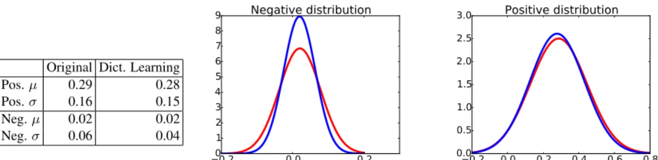
Our interpretation is that dictionary learning decreases the impact of features extracted from clutter patches be-cause they are not common across the image collection; i.e., it favors the frequent visual patterns in the image collec-tion. To explore this phenomenon further, we plot the dis-tribution of matching and non-matching vector similarities from Oxford5k using the original global descriptors. We repeat the same process using the reconstructed similarities from dictionary learning. As we see in Figure 2, both recon-structed similarity distributions have a lower variance than the original distributions. This is especially true for the non-matching distribution. This variance reduction increases the separation between the distributions, which translates to the better performance of our dictionary learning method. Sparsity of H is controlled by parameterm in dictionary learning (see Section 3.2). This is an important factor in the complexity ratioρ. The ratio between m and d contributes toρ independently from M . It is possible to set this ratio to a small value to eliminate its influence.
We compute a dictionary ofM atoms and we calculate several matrices H by applying OMP with differentm. We plot the retrieval performance for differentm and M in Fig-ure 3. In most cases, the performance does not vary much w.r.t.m. The biggest difference is observed for Oxford105k where largerm leads to better performance for small M . The dimensionality of the vectors is an important factor affecting the overall complexity. Lower dimensionality
im-Original Dict. Learning Pos.µ 0.29 0.28 Pos.σ 0.16 0.15 Neg.µ 0.02 0.02 Neg.σ 0.06 0.04 0.2 0.0 0.2 0 1 2 3 4 5 6 7 8 9 Negative distribution 0.2 0.0 0.2 0.4 0.6 0.8 0.0 0.5 1.0 1.5 2.0 2.5 3.0 Positive distribution
Figure 2. Distributions of matching and non-matching vector similarities from Oxford5k dataset. Red (blue) curves represent distributions of true (resp. reconstructed) similarities. The main improvement comes from the reduction of variance under the negative distribution.
m 25 1052 M/N 0.10 0.20 0.30 0.40 0.50 mAP 0.2 0.3 0.40.5 0.60.7 0.8
oxford5k
m 25 1052 M/N 0.02 0.04 0.06 0.08 mAP 0.0 0.1 0.20.3 0.40.5 0.6 0.7oxford105k
m 25 1052 M/N 0.10 0.20 0.30 0.40 mAP 0.45 0.500.55 0.60 0.650.70 0.75 0.800.85 0.90paris6k
m 25 1052 M/N 0.02 0.04 0.06 0.08 mAP 0.3 0.40.5 0.60.7 0.8 0.9paris106k
Figure 3. Retrieval performance with differentM and m. Varying m does not affect the performance in most cases, except for Oxford105k, where increasingm improves performance for small M .
plies lower complexity and less memory usage. Although our experiments up to now are done in what can be con-sidered as a low-dimensional feature space (d = 512), we evaluate our system with even smaller features, d = 256, in Figure 4. The results are similar to those ford = 512, although the accuracy of eigendecomposition increases at a slower rate for largeN .
The training stage computes Y and H and is performed only once and offline. However, it is important that this stage is scalable for updating the dictionary if needed. Ex-perimentally, a small number of iterations (≈ 100) is suf-ficient for dictionary learning. This does not require much training time. Using Mairal et al. ’s algorithm [19], we re-port the duration of the offline training on Figure 5. All ex-periments are done on a server with IntelrXeonrE5-2650 2.00GHz CPU and 32 cores. The training time is reasonable for all datasets, but it increases dramatically withM in large datasets. Other training procedures would be necessary for handling largeM and N .
Coresets, as explained in Section 3.3, reduce the training time even further for large datasets. Instead of using the entire dataset, we find a coreset C which represents the data with a few representatives vectors to train the dictionaries. We report results for coresets of different sizes in Table 1. Empirically, we achieve a similar performance by training on coresets of vectors. This allows us to train the dictionary for largerM in just a few minutes. Note that Paris106k has fast training time even without coresets. This is because the best performance for this dataset is obtained withM = 532, a rather small value. The drawback to using coresets
Oxford105k Paris106k
mAP Time mAP Time
|C| = N/10 60.1±1.1 14.6 78.3±1.0 1.8
|C| = N/5 62.1±1.2 16.9 79.2±0.8 2.3
|C| = N/2 62.7±0.4 23.9 79.5±0.4 3.3
X 65.5 45.5 81.2 5.3
Table 1. Performance and training time (in minutes) using coresets to train the dictionary.M is set to 5, 257 and 532 for Oxford105k and Paris105k respectively, andm = 50. Each experiment is run 5 times, and we report the mean and the standard deviation.
is that H is less sparse: m = 50. This results in the same performance but slightly higher complexity.
The search time is the average number of seconds to re-spond to a query. Although comparing vector operations is reliable in general, we also include the actual timings. Ex-haustive search takes 0.029s on Oxford105k and 0.03s on Paris106k (average per query). Our method takes 0.003s on Oxford105k (M = 5, 257), and 0.001s on Paris106k (M = 532), with higher mAP than exhaustive search.
5.3. Comparison with other methods
We compare our system with other image retrieval ap-proaches. First we compare with the popular FLANN tool-box [20] using Oxford105k and R-MAC features. We set the target precision to 0.95 and use the “autotuned” setting of FLANN, which optimizes the indexing structure based on the data. We repeat this experiment 5 times. The aver-age speed-up ratio provided by the algorithm is 1.05, which corresponds to a complexity ratio of 0.95. In other words, FLANN is ineffective for these R-MAC descriptors, most
0.2 0.4 0.6 0.8 0.1 0.2 0.3 0.4 0.5 mAP Complexity Ratio Oxford5k Base Eig DL LSH 0.1 0.2 0.3 0.4 0.5 0.6 0 0.1 0.2 0.3 0.4 0.5 mAP Complexity Ratio Oxford105k Base Eig DL LSH 0.2 0.4 0.6 0.8 0.1 0.2 0.3 0.4 0.5 mAP Complexity Ratio Paris6k Base Eig DL LSH 0.1 0.2 0.3 0.4 0.5 0.6 0.7 0 0.1 0.2 0.3 0.4 0.5 mAP Complexity Ratio Paris106k Base Eig DL LSH
Figure 4. Retrieval performance using smaller features:d = 256.
0 0.5 1 1.5 2 2.5 0.1 0.2 0.3 0.4 0.5 Minutes Complexity Ratio Oxford5k DL 20 0 40 60 80 100 120 140 160 180 0 0.05 0.1 0.15 0.2 Minutes Complexity Ratio Oxford105k DL 0 0.5 1 1.5 2 2.5 3 3.5 0.1 0.2 0.3 0.4 0.5 Minutes Complexity Ratio Paris6k DL 0 20 40 60 80 100 120 140 160 180 0 0.05 0.1 0.15 0.2 Minutes Complexity Ratio Paris106k DL
Figure 5. Offline training time needed for dictionary learning with 100 iterations.
Mem. Ratio Holidays Oxford5k UKB
Exhaustive 1.0 77.1 67.4 3.63
Iscen et al. [11]-Kmeans 1.4 76.9 67.3 3.63
Iscen et al. [11]-Rand 1.4 75.8 62.0 3.63
Shi et al. [27] w/ bp. 1.4 75.5 64.4 3.63
Borges et al. [5] 1.0 59.2 59.9 3.43
LSH [6] 0.4 73.9 65.8 3.61
PCA 0.4 75.4 64.3 3.61
Shi et al. [27] w/o bp. 0.4 8.7 24.1 1.33
Ours - Eigen. 0.4 76.9 67.7 3.63
Ours - Dict. Learn. 0.4 55.2 68.8 3.59
Table 2. Comparison in image retrieval for a given complexity ratio of 0.4. This experiment uses long t-embedding features (d = 8, 096). Eigendecomposition and dictionary learning gen-erally performs better at lower memory ratio.
Mem. Ratio Oxf5k Oxf105k Paris6k Paris106k
Exhaustive 1.0 66.9 61.6 83.0 75.7 [11]-Kmeans 1.1 65.6 61.2 79.7 75.7 [11]-Rand 1.1 25.1 43.7 21.2 44.4 [27] w/ bp. 1.1 15.4 28.1 18.7 37.7 [5] 1.0 8.5 22.7 8.2 18.9 LSH [6] 0.1 48.6 40.5 70.1 58.2 PCA 0.1 58.1 8.0 86.1 38.9 Ours-Eigen. 0.1 56.8 8.0 86.3 40.9 Ours-D.L. 0.1 73.7 65.5 85.3 78.9
Table 3. Comparison with R-MAC features (d = 512) and 0.1 complexity ratio.
likely due to their high intrinsic dimensionality (d = 512): as discussed by its authors [20], FLANN is not better than exhaustive search when applied to truly high-dimensional vectors. In contrast, our approach does not partition the feature space and does not suffer as much the curse of di-mensionality. Our descriptors are whitened for better per-formance [12], which tends to reduce the effectiveness of partitioning-based approaches.
Next we compare our method with other group testing
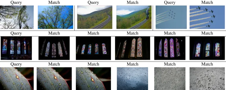
and indexing methods in the image retrieval literature. To have a fair comparison, we report the performance using the same high-dimensional features (d = 8, 064), same datasets, and the same complexity ratio as the group test-ing methods. Additionally, we also compare our scores to a dictionary learning-based hashing method [5], LSH [6] and PCA, where dimensionality of vectors is reduced such that d′ = 0.4d. Table 2 shows the comparison for a fixed complexity ratio. We outline two observations. First, eigen-decomposition works well in these experiments. This is es-pecially true for the Holidays dataset where N = 1, 491 andd = 8, 064; large M can be used while keeping the complexity ratio low since N < d. This is clearly a sce-nario where it is plausible to use the eigendecomposition approach. Second, dictionary learning performs poorly for Holidays. This dataset contains only1, 491 images, which constrains the size of the dictionaryM to be small and pre-vents sparsity: the best parameters (via cross-validation) are found to be M = 519 and m = 409, giving ρ = 0.4. Note that this experiment uses long t-embedding descriptors (d = 8, 096) in small and mid-scale datasets. Most likely, these features have low intrinsic dimensionality, and PCA and LSH are thus favored. Table 3 uses shorter R-MAC features (d = 512) for comparison. The increase in perfor-mance is more significant, especially for large datasets. Yahoo100M is a recently released large-scale dataset con-sisting of approximately 100M images. Since there is no manually annotated ground-truth, we use the following evaluation protocol: a dataset vector is considered to match the query if its cosine similarity is at least0.5. There are 112 queries randomly selected from the dataset. Each query has between 2 and 96 matches, and 11.4 matches on average. Table 5.2 shows visual examples of queries and matches.
This dataset is split into chunks ofN′ = 100k images. We run dictionary learning and OMP independently to learn matrices Y and H for each chunk, settingM′ = N′/100 and m = 100. Overall, it results in M = N/100. We
Query Match Query Match Query Match
Query Match Match Match Match Match
Query Match Match Match Match Match
Table 4. Some examples of match and query in Yahoo100M dataset. Two vectors are considered a match if their similarity is above 0.5.
M = N/200 M = N/100 M = N/50
mAP ρ mAP ρ mAP ρ
m = 100 85.7 0.105 89.4 0.11 92.8 0.12
m = 50 81.0 0.055 84.7 0.06 87.4 0.07
m = 20 61.8 0.025 71.4 0.03 78.2 0.04
Table 5. Performance (mAP) and complexity ratio (ρ) in Ya-hoo100M for differentM and m.
can perform this offline stage in parallel. At query time, we pool scores from each chunk together and sort them to determine a final ranking. When we evaluate the retrieval performance, we obtain a mAP of 89.4 withρ ≈ 1/10. This is a significant increase compared to running the same setup with LSH, which results in a mAP of70.9. Furthermore, it is still possible for the dictionary learning approach to obtain very good performance withρ < 1/10 by setting M andm to smaller values as shown in Table 5.3.
Similar to other datasets, we apply coresets for the Ya-hoo100M dataset. We learn a coreset for each chunk sepa-rately, which makes its calculation feasible. We set|C| = N/2, m = 100 and M = N/100, and obtain a mAP of 87.9 compared to a mAP of 89.4 using the entire chunks. Compatibility with coding methods. One of the main strengths of our method is its complementarity with other popular coding strategies in computer vision. We com-bine our method with PQ-codes [14] as explained in Sec-tion 4. We useℓ = d/b subvectors for different values of b andQ = 256 codewords per each subquantizer (except for Paris6k whereQ = 16 due to small M ). This reduces the termO(M × d) by a factor of b if we neglect the fixed cost of complexity of building the lookup table.
Table 6 shows the difference of performance with and without PQ-codes. Observe that the performance remains almost the same forb = 8. The compression factor by
PQ-Baseline Our Method b = 8 b = 64
Oxford5k 66.9 73.4 73.1 72.9
Paris6k 83.0 88.1 87.7 85.6
Oxford105k 61.6 65.5 63.1 30.4
Paris106k 75.7 81.2 80.9 76.8
Table 6. Combination of our method with PQ-codes. We use M = 350 for Oxford5k, M = 30 for Paris6k, M = 5257 for Oxford105k, andM = 532 for Paris106k.
code is significant (8 floats replaced by 1 byte).
6. Conclusion
This paper lowers the complexity of image search by re-ducing the number of vector comparisons. We formulate the image search problem as a matrix factorization prob-lem, which can be solved using eigendecomposition or dic-tionary learning. We show that the former is a plausible option for small datasets, whereas the latter can be ap-plied for large-scale problems in general. When apap-plied to real datasets comprising up to 108
images, our frame-work achieves a comparable, and sometimes better perfor-mance, than exhaustive search within a fraction of complex-ity. It is worth noting that this approach is complementary to other indexing/approximated similarity approaches such that it can be combined to further increase efficiency.
Acknowledgments
This work was supported, in part, by the Natural Sci-ences and Engineering Research Council of Canada through grant RGPAS 429296-12, and by the French National Project IDFRAud (ANR-14-CE28-0012). Portions of this work were completed while the first author was visiting McGill University.
References
[1] P. K. Agarwal, S. Har-Peled, and K. R. Varadarajan. Ap-proximating extent measures of points. Journal of the ACM, 51(4):606–635, 2004.
[2] R. Arandjelovi´c and A. Zisserman. Extremely low bit-rate nearest neighbor search using a set compression tree. IEEE Trans. PAMI, 2014.
[3] A. Babenko and V. Lempitsky. The inverted multi-index. In CVPR, June 2012.
[4] A. Babenko, A. Slesarev, A. Chigorin, and V. Lempitsky. Neural codes for image retrieval. In ECCV, 2014.
[5] P. Borges, A. Mour˜ao, and J. Magalh˜aes. High-dimensional indexing by sparse approximation. In Proceedings of the 5th ACM on International Conference on Multimedia Retrieval, 2015.
[6] M. S. Charikar. Similarity estimation techniques from round-ing algorithms. In STOC, pages 380–388, May 2002. [7] G. M. Davis, S. G. Mallat, and Z. Zhang. Adaptive
time-frequency decompositions with matching pursuit. In SPIE’s International Symposium on Optical Engineering and Pho-tonics in Aerospace Sensing, pages 402–413, 1994. [8] W. Dong, M. Charikar, and K. Li. Asymmetric
dis-tance estimation with sketches for similarity search in high-dimensional spaces. In SIGIR, pages 123–130, July 2008. [9] E. Elhamifar, G. Sapiro, and R. Vidal. See all by looking at
a few: Sparse modeling for finding representative objects. In CVPR, 2012.
[10] D. Feldman, M. Feigin, and N. Sochen. Learning big (image) data via coresets for dictionaries. Journal of Mathematical Imaging and Vision, 46(3):276–291, 2013.
[11] A. Iscen, T. Furon, V. Gripon, M. Rabbat, and H. J´egou. Memory vectors for similarity search in high-dimensional spaces. arXiv preprint arXiv:1412.3328, 2014.
[12] H. J´egou and O. Chum. Negative evidences and co-occurrences in image retrieval: The benefit of PCA and whitening. In ECCV, October 2012.
[13] H. J´egou, M. Douze, and C. Schmid. Hamming embedding and weak geometric consistency for large scale image search. In ECCV, October 2008.
[14] H. J´egou, M. Douze, and C. Schmid. Product quantization for nearest neighbor search. IEEE Trans. PAMI, 33(1):117– 128, January 2011.
[15] H. J´egou, M. Douze, C. Schmid, and P. P´erez. Aggregating local descriptors into a compact image representation. In CVPR, June 2010.
[16] H. J´egou and A. Zisserman. Triangulation embedding and democratic kernels for image search. In CVPR, June 2014. [17] D. G. Lowe. Distinctive image features from scale-invariant
keypoints. IJCV, 60(2):91–110, 2004.
[18] J. Mairal, F. Bach, and J. Ponce. Sparse modeling for im-age and vision processing. arXiv preprint arXiv:1411.3230, 2014.
[19] J. Mairal, F. Bach, J. Ponce, and G. Sapiro. Online learning for matrix factorization and sparse coding. The Journal of Machine Learning Research, 11:19–60, 2010.
[20] M. Muja and D. G. Lowe. Scalable nearest neighbor algo-rithms for high dimensional data. IEEE Trans. PAMI, 36, 2014.
[21] R. Negrel, D. Picard, and P.-H. Gosselin. Dimensional-ity reduction of visual features using sparse projectors for content-based image retrieval. In ICIP 2014, pages 2192– 2196, 2014.
[22] D. Nist´er and H. Stew´enius. Scalable recognition with a vo-cabulary tree. In CVPR, pages 2161–2168, June 2006. [23] Y. C. Pati, R. Rezaiifar, and P. Krishnaprasad.
Orthog-onal matching pursuit: Recursive function approximation with applications to wavelet decomposition. In ASILOMAR, pages 40–44, 1993.
[24] F. Perronnin and C. R. Dance. Fisher kernels on visual vo-cabularies for image categorization. In CVPR, June 2007. [25] J. Philbin, O. Chum, M. Isard, J. Sivic, and A.
Zisser-man. Object retrieval with large vocabularies and fast spatial matching. In CVPR, June 2007.
[26] J. Philbin, O. Chum, M. Isard, J. Sivic, and A. Zisserman. Lost in quantization: Improving particular object retrieval in large scale image databases. In CVPR, June 2008.
[27] M. Shi, T. Furon, and H. J´egou. A group testing framework for similarity search in high-dimensional spaces. In ACM Multimedia, November 2014.
[28] E. Spyromitros-Xioufis, S. Papadopoulos, I. Kompatsiaris, G. Tsoumakas, and I. Vlahavas. A comprehensive study over VLAD and product quantization in large-scale image retrieval. IEEE Trans. on Multimedia, 2014.
[29] B. Thomee, D. A. Shamma, G. Friedland, B. Elizalde, K. Ni, D. Poland, D. Borth, and L.-J. Li. Yfcc100m: The new data in multimedia research. Commun. ACM, 59(2), 2016. [30] G. Tolias, R. Sicre, and H. J´egou. Particular object retrieval
with integral max-pooling of cnn activations. ICLR, 2016. [31] R. Weber, H.-J. Schek, and S. Blott. A quantitative
analy-sis and performance study for similarity-search methods in high-dimensional spaces. In VLDB, pages 194–205, 1998. [32] Y. Weiss, A. Torralba, and R. Fergus. Spectral hashing. In
![Figure 1. Comparison of eigendecomposition, dictionary learning (DL), and LSH [6]. DL gives better performance, all the more so as the dataset is large](https://thumb-eu.123doks.com/thumbv2/123doknet/12450445.336166/6.918.84.817.107.225/figure-comparison-eigendecomposition-dictionary-learning-better-performance-dataset.webp)