FACULTY OF ECONOMICS AND MANAGEMENT
AGRARIAN PERSPECTIVES XXIX.
TRENDS AND CHALLENGES OF AGRARIAN SECTOR
PROCEEDINGS
of the 29
thInternational Scientific Conference
September 16 - 17, 2020
Prague, Czech Republic
Czech University of Life Sciences Prague Faculty of Economics and Management © 2020
PROCEEDINGS - of the 29th International Scientific Conference Agrarian Perspectives XXIX. Trends
and Challenges of Agrarian Sector
Publication is not a subject of language check.
Czech University of Life Sciences Prague, Faculty of Economics and Management
Agrarian perspectives XXIX. Trends and Challenges of Agrarian Sector
Programme committee
Martin Pelikán (CZU Prague) Milan Houška (CZU Prague) Jan Hučko (CZU Prague) Michal Lošťák (CZU Prague) Mansoor Maitah (CZU Prague) Michal Malý (CZU Prague) Ludmila Pánková (CZU Prague)
Peter Bielik (Slovak University of Agriculture in Nitra) Jarosław Gołębiewski (Warsaw University of Life Sciences) Elena Horská (Slovak University of Agriculture in Nitra) Irina Kharcheva (Russian Timiryazev State Agrarian University) Thomas L. Payne (University of Missouri)
Dagmar Škodová Parmová (University of South Bohemia in Ceske Budejovice)
Pavel Žufan (Mendel University in Brno)
Organizing Committee
Head: Ludmila Pánková Members: Renata Aulová
Hana Čtyroká Michal Hruška Jan Hučko Jiří Jiral Michal Malý Pavel Moulis Editorial Board
Chief Editor: Karel Tomšík (CZU Prague) Members: Martina Fejfarová (CZU Prague)
Heinrich Hockmann (IAMO) Milan Houška (CZU Prague)
Jochen Kantelhardt (Austrian Society of Agricultural Economics) Michal Malý (CZU Prague)
Walenty Poczta (Poznań University of Life Sciences) Libuše Svatošová (CZU Prague)
Hans Karl Wytrzens (University of Natural and Life Sciences in Vienna) Technical editor: Jiří Jiral, Tomáš Maier, Hana Čtyroká, Lenka Rumánková, Pavel Kotyza
Reviewers: Gabriela Kukalová, Pavlína Hálová, Jiří Mach, Věra Majerová, Michal Malý, Lukáš Moravec, Ladislav Pilař, Radka Procházková, Stanislav Rojík, Elizbar Rodonaia, Pavel Šimek, Miloš Ulman
Publisher
Czech University of Life Sciences Prague Kamýcká 129, Prague 6, Czech Republic
ETHICS GUIDELINES
The conference AGRARIAN PERSPECTIVES is committed to the highest ethics standards. All authors, reviewers, and editors are required to follow the following ethical principles. In case of any doubts do not hesitate to contact the editors of the conference AGRARIAN PERSPECTIVES.
The editors (co-editors) have the following responsibilities:
• The editor(s) clearly identify contributions that are fully with the scope and aim of the conference AGRARIAN PERSPECTIVES. The editor(s) should treat all contributions fairly without any favour of prejudice. The editor(s) only authorise for review and publication content of the highest quality.
• The editor(s) should recuse himself or herself from processing any contribution if the editor(s) have any conflict of interest with any of the authors or institutions related to the manuscripts.
• The editor(s) should provide advice to the author(s) during the submission process whennecessary.
• The editor(s) should be transparent with regards to the review and publication process withan appropriate care that individuals will not be identified when it is inappropriate to so do.
• The editor(s) should not use any parts or data of the submitted contribution for his or her ownfuture research as the submitted contribution is not published yet.
• The editor(s) should respond immediately and take reasonable action when ethical problemsoccur concerning a submitted or a published contribution. The editor(s) should immediatelycontact and consult these issues with the author(s).
The author(s) have the following responsibilities:
The author(s) ensure that submitted contribution is original, prepared to a high scholarly standard and fully referenced using the prescribed referencing convention. Therefore, the author(s) should carefully read the instructions for authors published on the website of the conference AGRARIAN PERSPECTIVES.
• The author(s) should not submit similar contributions (or contributions essentially describingthe same subject matter) to multiple conferences or journals. Furthermore, the author(s) should not submit any contribution previously published anywhere to the conferences orjournals for consideration.
• The author(s) are represented accurately and other appropriate acknowledgements are clearlystated including sources of funding if any.
• The author(s) state the source of all data used in the submitted contribution and how the datawas acquired. Moreover, the author(s) should clarify that all the data has been acquiredfollowing ethical research standards.
• The author(s) recognise that the editors of the conference AGRARIAN PERSPECTIVES. have the final decision to publish the submitted, reviewed and accepted contribution.
• The author(s) should immediately inform the editor(s) of any obvious error(s) in his or heraccepted contribution. The author(s) should cooperate with the editor(s) in retraction orcorrection of the contribution.
The reviewers have the following responsibilities:
• The reviewer(s) who feel unqualified to review the assigned contribution or if the reviewer(s) feel that cannot meet the deadline for completion of the review should immediately notify theeditor(s).
• The reviewer(s) should inform the editor(s) if there is any possible conflict of interest relatedto the assigned contribution. Specifically, the reviewer(s) should avoid reviewing anycontribution authored or co-authored by a person with whom the reviewer(s) has an obviouspersonal or academic relationship.
• The reviewer(s) should treat the contribution in a confidential manner. Read the contributionwith appropriate care and attention and use his or her best efforts to be constructively critical.The contribution should not be discussed with others except those authorized by the editor(s).
• The reviewer(s) should agree to review a reasonable number of contributions.
• The reviewer(s) should not use any parts or data of the reviewed contribution for his or herown future research as the reviewing contribution is not published yet.
• The reviewer(s) should immediately notify the editor(s) of any similarities between thereviewing contribution and another manuscript either published or under consideration byanother conference or journal.
Any report of possible ethics conflicts is a major issue for the conference AGRARIAN PERSPECTIVES. All ethics conflicts reported by reviewer(s), editor(s), co-editor(s) or reader(s) will be immediatelyinvestigated by the editors of the conference.
If misconduct has been committed the published contribution will be withdrawn. In addition, the author(s) may be excluded from having any future contribution reviewed by the conference AGRARIAN PERSPECTIVES.
FOREWORD
Agriculture, one of the oldest undertakings in recorded human history, still remains a strategic and integral part of every economy on earth. The 21st century, which has been characterized by turbulent changes in in every aspect of life, has brought a number of new challenges to the agricultural sector. It is not only the world's rapidly rising population and increasing demand on food supplies, but the sustainability of agricultural production that is closely intertwined with environmental and social requirements. The answers to these complex challenges require new and unorthodox approaches. The implementation of the latest scientific research findings, as well as comprehensive problem-solving utilizing the knowledge of various disciplines will be necessary to address the issues that currently face the agrarian sector.
Scientific conferences and professional seminars are an ideal platform for sharing opinions, experiences and the latest information in response to current challenges. The international scientific conference “Agrarian Perspectives”, organized by the Faculty of Economics and Management at the Czech University of Life Sciences Prague, has a long tradition in this regard that began in 1992. Since that time, the conference has become popular among scientists and experts from all around the world.
The 29th annual “Agrarian Perspectives” conference, held on the 16th and 17th of September 2020, will be focused on the topic of “Trends and Challenges in the Agrarian Sector”. Although the conference will not be held in its traditional format due to the current pandemic, the interest of the participants clearly demonstrates the usefulness and significance of this scientific meeting.
We strongly feel that the 29th annual Agrarian Perspectives conference will create an inspirational framework for all of the participants and contribute to the further development and expansion of agricultural research.
Karel Tomšík
Vice-dean for International relations
THE RELATIONSHIP BETWEEN CARBON DIOXIDE
EMISSIONS, ELECTRICITY CONSUMPTION,
AND ECONOMIC GROWTH IN SYRIA
Ahmed Altouma
Department of Economics, Faculty of Economics and Management, CULS Prague, Czech Republic
altouma@pef.czu.cz
Annotation: The 21st century has seen environmental degradation as one of the main challenges
experienced today. Syria, which is in a peculiar situation due to the ongoing war, is not exempt from this predicament. The objective of this article is to examine the relationship among carbon dioxide, electricity consumption, and economic growth for the time 1971 to 2014. In reaching this objective, the paper applied a cointegration test (which was done after the ARDL long- run bounds Test) and found the existence of cointegration amongst the variables, which was significant and adjusted to long-run equilibrium at -0.94 as expected consumption of electricity and economic growth all have a positive increment towards carbon dioxide emissions. These raise concern amongst policymakers who need to build environmentally friendly means of energy use and economic activities.
Key words: Carbon dioxide emissions, electricity consumption, economic growth, Syria. JEL classification: O13, F43
1. Introduction
There is no doubt that countries are striving for economic growth, achieving their goals in development, devoting all possible efforts to that. They sometimes overlook the environmental impacts of this growth. This issue gave continuous importance to navigating the relationship between environmental risks and economic variables and making them a major arrangement, decade after decade. (Ali, and de Oliveira, 2018).
Through the literature, the researchers developed three categories for the relationship between environmental pollutants and the economy (Heil, and Selden, 1999). The first one discusses the link between environmental pollutants and economic growth; in other words, it tests the Kuznets environmental curve. The second is economic development and energy consumption. The third is a common approach to both scenarios.
Andto understand the relationship between economic development and environment pollutants, both Dinda (2004) and Stern (2004) explain Kuznets curve model, the model has three stages. In the first stage, countries are working to increase economic growth and accompanied by energy consumption. Whereas countries use fossil energy to provide fair prices. Using this type of energy increases your CO2 emissions. In the second stage, despite the countries
According to IPCC, carbon dioxide emissions are the most prominent of these environmental hazards affecting climate change. IPCC has determined the distribution of global greenhouse gas emissions for the year 2010 at 25% for electricity and heat production, 24% for agriculture, forestry, and other land uses, 14% for transportation, 6% for buildings, and the remaining 10%. Mainly goes to fuel extraction, refining, treatment, and transportation.
According to the global carbon project, china tops the list of countries most contributing to carbon dioxide emissions, followed by the United States, India, and Russia.
In the past decade, Macao, Libya, Nauru, Ireland, and Northern Marian Islands and Rwanda have alternated over the pyramid of GDP growth countries. Where each of Macao, Libya, and Nauru remained for two years and one year for others according to the World Bank database.
In the past decade, China's consumption of electricity increased to 170% compared to 2010 as the most consumer of electricity globally, while the United States succeeded in maintaining almost the same consumption to remain second according to Global Energy Statistical yearbook, 2019.
Syria, like other countries in the Middle East, has worked to raise the economic growth, and after the crisis began in Syria in March 2011, the economic growth started to fall and reached the bottom in 2012 and 2013 in -26.3%. Then it started increasing and recovering until it reached -1.460% in 2017 according to ceicdata database. In regard to the consumption of electrical energy for the Syrian citizen's, It isn’t considered high compared to other countries of the world, with an average of 989 kWh per year per person according to the CIA, the World Factbook in the 2014 update.
Twenty-five conferences of parties were held starting in the nineties under the umbrella of the United Nations, which permeates the adoption of the Kyoto Protocol in 1997 which entered into force in 2005. However, the failure to reach an agreement binding on all parties continued until 2011, when an important shift occurred through the approval of a legally binding deal by all countries in 2015. All negotiations culminated in the Paris Climate Agreement, which was ratified by consensus of delegations.
Since the relationship between economic development and environmental pollutants was presented, many studies have discussed this relationship. Some researchers studied a single developing or developed country like Mikayilov, Galeotti, and Hasanov (2018) study about Azerbaijan. Some took a group of countries that have ties such as MENA countries like Farhani (2013).
Magazzino (2015) studied the Italian experience between 1970 and 2006 among economic growth, CO2 emissions, and energy consumption to examine the relationship between them by using Toda-Yamamoto approach and Granger causality test. Farhani (2013) studied the same variables as panel data for 12 MENA countries from 1975 till 2008 by using Pedroni cointegration test, Granger causality test, DOLS, and FMOLS to find linkages among the studied variables. Odugbesan and Murad (2019) added urbanization to the studied variables. The study discussed variables between 1993 and 2014 for 23 Sub-Saharan African countries by using pooled OLS regression test and fixed/random effect model. The purpose of this study was to explain interacting the combination of the studied variables. Mikayilov, Galeotti, and Hasanov (2018) investigated the relationship between economic growth and CO2 emissions
for the case study of Azerbaijan between 1992 and 2013 by implementing Johansen cointegration approach, ARDLBT, DOLS, FMOLS, and CCR. Bouznit and Pablo-Romero (2016) which talked about Algeria between 1970, 2010 using ARDL to examine the relationship between CO2 emissions and economic growth in Algeria, taking into account imports and exports in addition to energy use and electricity consumption. Shaari (2017) study which aims to investigate the effects of both electricity consumption and economic growth on carbon dioxide emission between 1971 to 2013 in Malaysia
This study consists of four parts. A theoretical discussion of the types of relationship between environmental pollutants and the economy and the form of the relationship according to Kuznets' environmental curve. It is followed by subtracting the main cause of global warming and distributing emissions according to industries in percentages. In addition, data is presented and explained regarding research variables globally in the last decade. The most important conferences related to climate change were discussed, and the purpose of the study was clarified. Besides, reviewing some previous studies discussed the same variables. The second section of the running paper is a description of the methods used. In the third part of the study, the results are presented and discussed with the results of previous studies. The last part of this study shows a summary of the study and the proposed topics for future studies.
2. Materials and Methods
Data set used in this study includes the period 1971-2014, and analyses have been studied on an annual data basis. CO2 emissions data have obtained from the world bank database as well as both economic growth from 1971 until 2007 have taken from the same source while years data from 2008 till 2014 have obtained from ceicdata database. While the electricity consumption data have obtained from trading economics data base. The researcher used both Excel 2010 and Eviews 11 for arranging the data and implementation of econometric analyses. Our empirical model examines the relationship among economic growth, and electricity consumption. The functional link between these variables yields:
CO = f(GDPt, ECt) (1)
Where, CO2, GDP, EC represent carbon dioxide emissions, economic growth, and electricity consumption.
The natural logarithmic transformation of Eq. (1) yields the following equation:
LnCO2 = α0 + α1LnGDPt +α2LnECt (2)
Where α0 = Intercept; α1,α2 are coefficients
In this paper, researcher uses ARDL cointegration approach to investigate the long-run relationship amongst CO2 emissions, economic growth, and electricity consumption.
H0: Series is not stationary (There is unit root). H1: Series is stationary (There is no unit root).
ARDL approach, the Autoregressive Distributed Lag is a cointegration test for examining long-run relationship that suggested by Persan and Pesaran (1997). We use this approach when dealing with variables that are I (0) or I (1) or fractionally integrated. Long run relationship of the series is acceptable when F-statistic exceeds the critical value band. The ARDL framework of Equation 3 of the model is as follows:
∆LnCO2t = a0 + ∑ a1i∆LnCO2t − 1 + ∑ a2i∆LnGDPt − 1 + ∑ a3i∆LnECt − 1 + λ ECMt − 1 (3) According to Woodridge (2004), the Model needs some extra tests for examining the quality of it. based on that, diagnostic tests particularly will be implemented for this purpose and mainly for the error term of the model. These tests included mainly the presence of autocorrelation in the error term, homoskedasticity, and for normality. H0 indicates the absence of serial correlation, heteroskedasticity, and the presence of normality. Moreover, for checking the model’s level of stability, the Cusum of squared test has done.
3. Results and discussion
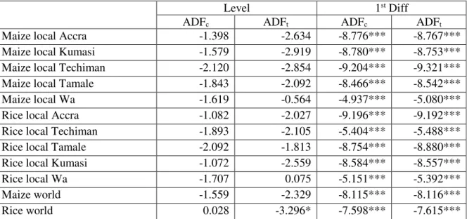
In this empirical study, we used Augmented Dickey-Fuller Stationary unit root tests to check for the integration order of each variable. Researcher has used the ADF unit root test to check for stationarity. The results in Table 1 indicate that all variables except GDP growth are non-stationary at their level form and stationery at their first differences.
Table 1. UNIT ROOT RESULTS (ADF RESULTS)
Variable Test Level 1st difference
Statistic 5% critical Statistic 5% critical
CO2 emissions (Kt) Cons -2.3988 -2.9314 -6.2191 -2.9332
Cons & Trend -0.0908 -3.5181 -7.8305 -3.5208
None 1.1897 -1.9487 -5.9797 -1.9489
Electric power consumption (kWh
per capita)
Cons -1.9038 -2.9332 -4.1871 -2.9332
Cons & Trend 0.7766 -3.5181 -4.7572 -3.5208
None 1.1590 -1.9489 -3.9335 -1.9489
GDP growth Cons -4.2807 -2.9332 - -
Cons & Trend -4.7250 -3.5208 - -
None 1.1590 -1.9489 - -
Source: Author computations (2020)
In this study, the computed F – statistic, which is greater than the upper critical values of entire significant levels. The guideline says that if the computed F- statistic is greater than I1 critical values, the results showed a cointegration status.
Table 2. ARDL LONG – RUN BOUNDS TEST OF COINTEGRATION F-Bounds Test Null Hypothesis: No levels relationship
Test Statistic Value Signif. I(0) I(1)
Asymptotic: n=1000 F-statistic 19.04137 10% 3.17 4.14 k 2 5% 3.79 4.85 2.5% 4.41 5.52 1% 5.15 6.36
With optimal lag length selected, the long – run equation was estimated using the ordinary least squares, its residue (error correction term) determined, and the error correction model estimated. The error correction model results are indicated in Table 4 below:
Table 3. VAR Lag Order Selection Criteria
Endogenous variables: LCO2 Exogenous variables: C LEC LGDP
Sample: 1971 2014 Included observations: 40
Lag LogL LR FPE AIC SC HQ
0 19.3404 NA 0.0259 -0.8170 -0.6904 -0.7712
1 31.5606 21.9963* 0.0148 -1.3780 -1.2091* -1.3170*
2 32.6173 1.8493 0.0147* -1.3809* -1.1698 -1.3045
3 32.6427 0.0432 0.0155 -1.3321 -1.0788 -1.2405
* indicates lag order selected by the criterion
LR: sequential modified LR test statistic (each test at 5% level) FPE: Final prediction error
AIC: Akaike information criterion SC: Schwarz information criterion HQ: Hannan-Quinn information criterion
Source: Author computations (2020)
The results in table 4 indicate that all estimated coefficients are statistically significant. Based on that, both economic growth and electricity consumption lead to increase in CO2 emissions. Moreover, the estimates indicate that 1% increase in economic growth leads to higher CO2 emissions by 0.61%, as well as 1% increase in electricity consumption leads to higher CO2 emissions by 0.37%.
Table 4. Long-run estimation results
Dependent variable Lco2
Variable Coefficie
nt
Std. Error t-Statistic Prob.
C 5.5348 1.0478 5.2829 0.0000
LEC 0.3765 0.1039 3.6249 0.0017
LGDP 0.6136 0.1146 5.3532 0.0000
Source: Authors computations (2020) Significance at 5 percent probability
As the results in Table 5 indicate, the effect of electricity consumption and economic growth on carbon emissions adjusted to long – run equilibrium at a speed of -0.94 and was significant. In addition, the coefficient of economic growth has a significant impact with a positive sign.
Table 5. Error correction model (ECM) for short-run elasticity ARDL
ARDL Error Correction Regression
Variable Coefficient Std. Error t-Statistic Prob.
C 5.5348 0.6981 7.9286 0.0000
D(LEC) -0.2184 0.2441 -0.8947 0.3816 D(LGDP) 0.1276 0.0240 5.3112 0.0000 CointEq(-1)* -0.9400 0.1186 -7.9270 0.0000
Table 6 shows the results of autocorrelation, heteroskedasticity, and abnormality. The tests indicate p – values of 0.5291, 0.1261, and 0.8235, respectively, which are all greater than 5 percent, which articulate the rejection of the N0.
Table 6. DIAGNOSTIC TESTS
Problem Test p-value
Autocorrelation Breusch-Godfrey LM 0.5291
Heteroskedasticity Breusch-Godfrey LM 0.1261 Normality Histogram (Jarque – Bera) 0.8235
Source: Author computations (2020) Significance at 5 percent probability
The figure below, which is cusum of squares, shows us stability.
Figure 1. Stability Test
Similar to the paper, Odugbesan and Murad (2019), Mikayilov, Galeotti, and Hasanov (2018) and Shaari (2017) research papers agreed with the results in regard to the cointegration. In contrast, Magazzino(2015) was non-cointegrated among the studied variables. Therefore, it can be concluded that there is a long run relationship among the variables in the first three studies.
Whereas Shaari (2017), Mikayilov, Galeotti, and Hasanov (2018) and this paper said that the increase in GDP leads to an increase in carbon emissions, Odugbesan and Murad (2019) indicated the opposite. With respect to the other variable, which changes from a study to another (the fixed variables usually economic growth and CO2 emissions), which is electricity consumption in this paper. Shaari (2017) and Bouznit and Pablo-Romero (2016) studied the same extra variable and indicated that an increase in electricity consumption could cause carbon dioxide emission, which has found in this paper. Apart from the long-run relationship, Shaari (2017) results show that economic growth and electricity consumption do not have any effect on carbon dioxide emissions on the short-run. In the running study, there is only effect between economic growth and carbon dioxide emission. While in Farhani (2013), there is an effect between CO2 emissions and renewable energy consumption.
4. Conclusion
This study aims to examine the relationship among electricity consumption and economic growth on carbon dioxide emission in Syria from 1971 to 2014. The analyses started with the unit root test, and the results showed that the studied variables used are stationary. Part of them are stationary at the form level and others at the first difference. Subsequently, the ARDL bound testing approach was implemented. The results indicated that in the long run,
-0.4 -0.2 0.0 0.2 0.4 0.6 0.8 1.0 1.2 1.4 1980 1985 1990 1995 2000 2005 2010
all variables are statistically significant, and each of them leads to lead to increasing CO2 emissions. In the short run, only economic growth has a significant impact with a positive sign. Policy makers can use these results as a justification to manage the electricity consumption and have environmentally friendly, sustainable electrical solutions
References
Ali, S. H. and de Oliveira, J. A. P. (2018), “Pollution and economic development: an empirical research review”, Environmental Research Letters, Bristol, vol. 13, no. 12, DOI 10.1088/1748-9326/aaeea7
Bouznit, M. and Pablo-Romero, M. D. P. (2016), CO2 emission and economic growth
in Algeria, Energy Policy, United Kingdom, vol. 96, pp. 93 – 104, ISSN 0301-4215, DOI 10.1016/j.enpol.2016.05.036
CEIC, Syria Real GDP Growth, 2020, [Online], Available: http://www.ceicdata.com/en/indicator/syria/real-gdp-growth ,[Accessed: 3 April. 2020]
Central Intelligence Agency, The World Factbook Archive, Middle East: Syria, 2015, [Online], Available: http://www.cia.gov/library/publications/the-world-factbook/geos/sy.html, [Accessed: 12 April. 2020]
Dinda, S. (2004), “Environmental Kuznets curve hypothesis: a survey". Ecological economics, vol.49, no. 4, pp. 431- 455, ISSN 0921-8009, DOI 10.1016/j.ecolecon.2004.02.011
Edenhofer, O. (2015), “Climate change 2014: mitigation of climate change”, vol. 3, Cambridge, Cambridge University Press, ISBN 978-1-107-05821-7
Farhani, S. (2013), “Renewable energy consumption, economic growth and CO2 emissions:
Evidence from selected MENA countries”, Energy Economics Letters, vol. 1, no. 2, pp. 24 – 41, E- ISSN 2308-2925
Global Carbon Project, CO2 emissions, 2019, [Online], Available: http://www.globalcarbonatlas.org/en/CO2-emissions, [Accessed: 1 April 2020]
Global Energy Statistical Yearbook, Electricity Consumption, 2019, [Online], Available: http://yearbook.enerdata.net/electricity/electricity-domestic-consumption-data.html,
[Accessed: 4 April. 2020]
Heil, M. T. and Selden, T. M. (1999), “Panel stationarity with structural breaks: carbon emissions and GDP”, Applied Economics Letters, vol. 6, E-ISSN 1466-4291, DOI 10.1080/135048599353384
IPCC, Intergovernmental Panel on Climate Change (2014), “Mitigation of climate change”, Contribution of working group III to the fifth assessment report
Magazzino, C. (2015), “Economic growth, CO2 emissions and energy use
in Israel”, International Journal of Sustainable Development & World Ecology, vol. 22, no. 1, pp. 89 - 97. ISSN 1350-4509, E-ISSN 1745-2627, DOI 10.1080/13504509.2014.991365 Mikayilov, J. I., Galeotti, M. and Hasanov, F. J. (2018), “The impact of economic growth on CO2 emissions in Azerbaijan”, Journal of Cleaner Production,vol. 197, pp. 1558 - 1572.
ISSN: 0959-6526, DOI 10.1016/j.jclepro.2018.06.269
Odugbesan, J. A. and Murad, B. (2019), “Economic Growth, CO2 Emissions, Energy
Consumptions and Urbanization in Sub-Sahargan Africa”, International Journal of Research in Social Sciences, vol. 9, no. 4, pp.635 – 653, ISSN 2454-4671. DOI 10.15640/jeds.v3n2a7 Pesaran, M. H. and Pesaran, B. (1997) “Working with Microfit 4.0: interactive econometric analysis; [Windows version]”, Oxford University Press,Oxford, United Kingdom.
Shaari, M. S., Razak, N. A. A. and Hasan-Basri, B. (2017), “The effects of electricity consumption and economic growth on Carbon Dioxide emission”, International Journal of Energy Economics and Policy, vol. 7, no. 4, pp. 287 - 290, ISSN 2146-4553
Stern, D. I. (2018), “The environmental Kuznets curve”, Companion to Environmental Studies”, vol. 49, no. 54, pp. 49 - 54. ROUTLEDGE in association with GSE Research, ISBN-13: 978-1138192201, ISBN-10: 1138192201
World Bank, GDP Growth, 2020, [Online], Available:
http://data.worldbank.org/indicator/NY.GDP.MKTP.KD.ZG, [Accessed: 6 April. 2020]. Yavuz, N. Ç. (2014), “CO2 emission, energy consumption, and economic growth for Turkey”:
Evidence from a cointegration test with a structural break”, Energy Sources, Part B: Economics, Planning, and Policy, vol. 9, no. 3, pp. 229 - 235. ISSN 1556-7249, E- ISSN 1556-7257, DOI 10.1080/15567249.2011.567222
THE INFLUENCE OF EXCHANGE RATE
ON ECONOMIC GROWTH: EVIDENCE FROM INDIA
Denim Umeshkumar Anajwala1 and Seth Nana Kwame Appiah-Kubi2
1, 2 Department of Economics, Faculty of Economics and Management, CULS Prague, Czech Republic 1denimanajwala91@gmail.com, 2appiah-kubi@pef.czu.cz
Annotation: In the globalization time frame conversion scale is the essential factor influencing
on financial development of each nation. This examination is embraced to inspect the effect of conversion scale on financial development of India during 1995 to 2018. As indicated by standard deviation it is seen that the GDP development is more predictable than conversion scale, loan cost and swelling rate during the examination time frame in India. The coefficient of connection 0.037426 demonstrates that the relationship between conversion standard and GDP development is sure however not critical. Be that as it may, the financing cost and expansion rate have reverse impact on monetary development of India during the examination time frame. It is watched structure the investigation that the conversion scale and loan cost has negative however not critical effect on financial development of India (Showing β = -0.0733305 and t = -0.4152 and β = -0.0113661, t = -0.07231 individually) during the examination time frame. In any case, it is discovered that the swelling rate has positive however not huge effect on financial development of India with (β = 0.0262511, t = 0.6584). Connection investigation shows positive, yet various relapse examination shows negative connection between swapping scale and GDP development in India during the investigation time frame.
Keywords: Exchange Rate, Inflation Rate, Interest Rate, GDP JEL classification: C01, F06, N01
1. Introduction
India has a free market and fare situated economy and is presently perhaps the best economy. There has been a significant enthusiasm among policymakers and specialists in India in understanding the effect of loan fee on India's monetary development. Be that as it may, writing of the exact econometric examination on monetary development changes as far as informational collections, econometric procedures, and regularly delivers clashing outcomes (Mussa, 1977). The nation's logical and innovative improvement is contended to be appealing to remote direct speculation.
Prior to moving to the exact examination, it is valuable to audit the writing on the nexus between genuine trade rates and monetary development, both hypothetical and experimental. Eichengreen (2008) offers an amazing survey of the discussion, including the job of conversion scale systems and swapping scale instability. Thusly, we center around later investigations and those closer to the target of this paper.
Jayachandran (2013) conducted a study on The Impact of Exchange rate on Trade and GDP for India a Study of Last four decade. This research has provided empirical estimates of the Economic relationship between Exchange Rate, Inflation, Government Revenue
Stotsky et al. (2012) examines the relationship between the foreign exchange regime and macroeconomic performance in India. They found that lagged inflation, broad money growth and fiscal position are key macroeconomic determinants of inflation. They observe that the actual exchange rate regime in place, with flexible and intermediate foreign exchange regimes producing lower inflation than the pegged exchange rate regime. They also found the evidence of a significant relationship between exchange rate movements and inflation, there is no evidence for full pass-through, both in the short and long run.
There is a direct relationship of inflation differential with domestic exchange rate (Alquist and Chinn, 2008). In other words, a higher domestic inflation relative to that of other nations results into depreciation of domestic currency (Soenen and Aggarwal, 1989). This is so because an increase in domestic inflation as compared to world inflation would increase the domestic demand for foreign commodities and lowers the foreigner and for domestic commodities, as more and more domestic consumer will shift toward foreign goods, supply of domestic currency in foreign exchange market will increase when these consumers will sell domestic currency for foreign currency (Babar and Khandare, 2012). This process would require depreciation of domestic currency to maintain the exchange rate as per the purchasing power theory. By same token, a decrease in domestic inflation as compared to world inflation causes appreciation of domestic currency. Therefore, the higher the inflation differential between domestic and foreign countries, the higher will be the depreciation of domestic currency and vice versa. This theory is called the Purchasing Power Parity. In another study Jain (2012) investigates the impact of bank rate policy of the Reserve Bank of India (RBI) and interest yield differentials between the India and the US securities. This paper also studied the impact of broad money supply and foreign exchange reserves.
Goyal (2010) concluded that exchange rate in India can be stabilized by raising interest rate. But even if the raising of interest rates lead to appreciation of exchange rate, the costs of raising interest rates in terms of large recession due fall in domestic consumption on account of reduced household borrowings, decline in business investment, corporate failures as many projects will turn unprofitable due to increase in discount rate, financial system bankruptcies or fragility may completely offset the benefits of an appreciated exchange rates So, there is cost of maintaining exchange rate by increasing the interest rate while the market determined exchange rates does not lead to such costs (Razzaque et al. 2017). However, in case of India, an increase in interest rates can lead to exchange rate appreciation without causing any adverse effects.
Higher government use account with enormous getting might contribute decidedly to the general execution of the economy. Government spending represses advancement. The private area continually arrangement for new thoughts, feelings and openings due to extreme fruition. For example, if government expands obtaining so as to back its enormous consumption, it will swarm out the private area, consequently decreasing private speculation or it might spend substantive sum on adjusting its current liabilities that can generally be utilized for venture. At the point when the administration acquires from another nation, financing cost in that nation goes up because an expansion popular for credits, subsequently pushing up the costs.
Moreover, in an offer to score modest notoriety and guarantee that they keep on staying in force, legislators and governments authorities here and there increment consumption and interest in useless undertakings or in products that the private area can create more proficiently. Along
these lines, government movement once in a while creates misallocation of assets and blocks the development of national yield (State Bank of India, 2012). In such cases, shockingly, rising open obligation for consistently mounting open use won't converted into significant development and advancement. This paper researches the impact of open obligation and open consumption independently on monetary development (GDP) in India.
While there have been various hypotheses and exact investigations the impacts of exchange on monetary development and its impact on general execution of the nation (Aggarwal, 1981), not many have tended to the significant issue of real estimations that plainly shows supportability. My goal here is to inspect whether loan fee is vigorous determinant of cross-country financial development.
This examination utilizes econometrics to investigations the effect of Interest rate on monetary development in India concentrating on today and tomorrow. This is on the grounds that econometrics is the unification of financial matters, arithmetic, and insights. This unification creates more than the total of its parts. Econometrics adds observational substance to monetary hypothesis enabling speculations to be tried and utilized for gauging and arrangement assessment.
2. Materials and Methods 2.1 Measurement of variables
The present study is based on secondary data collected from world data bank. The secondary data regarding GDP growth rate, Exchange rate, Interest rate and Inflation rate were collected from World Bank Data Publication. The required data collected for the period 1995 to 2018. For analysing growth performance of macroeconomic indicators average and compound annual growth rate has been used. The models used in this study are estimated using annual Indian data on some macro-economic indicators, which includes: Gross Domestic Products (GDP); Exchange Rate (EXR); Interest Rate (INR) and Inflation Rate (IFR) for the period 1995 to 2018. The correlation and multiple regression analysis of the ordinary least square (OLS) are used to determine the impact of exchange rate on economic growth of India. For determine the impact of selected macroeconomic indicators on economic growth of India the specifies model formulated as under;
GDP = f (EXR, INT, INF) GDP = β0 + β1 EXR + β2 INR + β3 INF
GDP = Gross Domestic Product EXR = Exchange Rate
INR = Interest Rate INF = Inflation Rate
with decrement of 0.34 occasions. While on a normal conversion scale was 48.92 per $ with increment of 1.8 occasions during 1995 to 2018 it was high than GDP development rate during this period. During the examination time frame on a normal Interest rate was 5.43 percent and Inflation rate was 6.88 percent. It is discovered that Interest rate and Inflation rates are diminished in 2018 with contrast with the underlying year 1995. It is seen from the information that the most noteworthy compound development rate recorded by Exchange rate for example 3.16 percent followed by GDP development rate -0.34 percent and Interest rate and Inflation rate recorded – 0.61 percent and – 1.24 percent compound yearly development rate individually during the investigation time frame. The Exchange rate developed during this examination period with a normal 3.46 percent every year while GDP developed by 8.62 percent, Interest rate and Inflation rate developed by – 1.24 percent every year during the investigation time frame. In this way, the conversion standard became so more than GDP development during the examination time frame. The Minimum and the most extreme trade rates were 32.43 and 68.39 separately. On account of this wide scattering of the conversion scale, the standard deviation 10.11 of the swapping scale from the mean conversion standard 48.92 was extremely high. Such high scattering of the information gives just feeble relationship and relapse coefficients. On account of swelling, the information was progressively dispersed.
Table 1. GDP growth rate, Exchange rate, Interest rate and Inflation rate in India
Year Exchange Rate Inflation Rate (%) Real Interest rate (%) GDP Growth Rate (%) 1995 32.43 10.22 5.86 7.57 1996 35.43 8.98 7.79 7.55 1997 36.31 7.16 6.91 4.05 1998 41.26 13.23 5.12 6.18 1999 43.05 4.67 9.19 8.85 2000 44.94 4.00 8.34 3.84 2001 47.19 3.78 8.59 4.82 2002 48.61 4.29 7.91 3.80 2003 46.58 3.80 7.30 7.86 2004 45.32 3.77 4.91 7.92 2005 44.10 4.24 4.85 7.92 2006 45.31 5.79 2.57 8.06 2007 41.35 6.37 5.68 7.66 2008 43.50 8.35 3.77 3.09 2009 48.40 10.88 4.80 7.86 2010 45.73 11.99 1.98 8.49 2011 46.67 8.86 1.32 5.24 2012 53.48 9.31 2.47 5.45 2013 58.60 10.91 3.86 6.38 2014 61.03 6.35 6.69 7.41 2015 64.15 5.87 7.55 7.99 2016 67.20 4.94 6.35 8.17 2017 65.12 2.49 5.46 7.17 2018 68.39 4.86 5.06 6.98 Average 48.92 6.88 5.43 6.68 Minimum 32.43 2.49 1.98 3.09 Maximum 68.39 13.23 9.19 8.85 CAGR 3.16 -3.05 0.61 -0.34 AAGR 3.46 3.32 1.24 8.62 Standard Deviation 10.11 3.04 2.57 1.70
The Minimum and the maximum exchange rates were 32.43 and 68.39 respectively. Because of this wide dispersion of the exchange rate, the standard deviation 10.11 of the exchange rate from the mean exchange rate 48.92 was very high. Such high dispersion of the data gives only weak correlation and regression coefficients. In the case of inflation, the data were more scattered.
The Minimum and the maximum rate of inflation were 2.49 percent and 13.23 percent respectively. However, the mean was 6.88 percent and the standard deviation was only 3.04 percent, which is more consistent. The data on growth rate of GDP were consistent. The Minimum and the maximum growth rate of GDP was 3.09 percent and 8.85 percent respectively. Average growth rate of GDP from 1995 to 2018 was 6.68 percent while the standard deviation was only 1.70 percent. The Minimum and the maximum rate of interest were 1.98 percent and 9.19 percent respectively. However, the mean was 5.43 percent and the standard deviation was only 2.57 percent, which is also more consistent. According to standard deviation it is observed that the GDP growth is more consistent than exchange rate, interest rate and inflation rate during the study period in India.
3. Results and Discussion
This chapter presents the results of the data analysis and discussion. The study provided two types of data analysis; namely descriptive analysis and inferential analysis. The descriptive analysis helps the study to describe the relevant aspects of the phenomena under consideration and provide detailed information about each relevant variable. For the inferential analysis, the panel regression was used. The first part highlights descriptive statistics. The second part focuses on the regression results of the fixed and random effect models. The last section presents the discussion of results.
3.1 Regression Results
Pearson coefficient of correlation between the exchange rate and the growth rate of GDP is 0.304 (30.4 percent) with a significance level of 0.149 or 14.9 percent. The coefficient of correlation 0.304 indicates that the correlation between exchange rate and GDP growth is negative but not significant. But the interest rate and inflation rate have inverse effect on economic growth of India during the study period. The correlation between interest rate and inflation is 0.906 and 0.165 respectively. This implies that the higher the interest rate and inflation rate the lower the level of gross domestic product of India.
Table 2. Correlation results GDP Growth Rate Exchange
Rate Interest Rate Inflation Rate GDP Growth Rate Correlation 1 -0.304 -0.025 0.165 Sig.(2-tailed) 0.149 0.906 0.441 N 24 24 24 24 Exchange Rate Correlation -0.304 1 -0.535 -0.008 Sig.(2-tailed) 0.149 0.007 0.969 N 24 24 24 24 Interest Rate Correlation -0.025 -0.535 1 -0.104 Sig.(2-tailed) 0.906 0.007 0.629 N 24 24 24 24 Inflation Rate Correlation 0.165 -0.008 -0.104 1 Sig.(2-tailed) 0.441 0.969 0.629
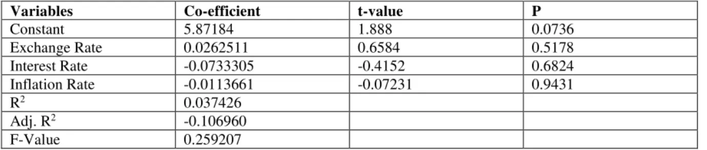
but not significant. The inflation rate shows that one percent decrease in inflation rate will 0.011 percent raise in economic growth of India. The value of R2 (coefficient of determination) in our model represents that 3.7 percent of the variations in the dependent variable (ln GDP) is due to independent variables included in the model.
Table 3. Summary of Regression Result of the model of the study
Variables Co-efficient t-value P
Constant 5.87184 1.888 0.0736 Exchange Rate 0.0262511 0.6584 0.5178 Interest Rate -0.0733305 -0.4152 0.6824 Inflation Rate -0.0113661 -0.07231 0.9431 R2 0.037426 Adj. R2 -0.106960 F-Value 0.259207
Source: Authors’ own calculation
4. Conclusion and Recommendation
This research study examined the impact of exchange rate on economic growth from 1995 to 2018. The result revealed that exchange rate has positive impact (β =0.0262511, t = 0.6584, Pns) this is not affirming previous studies that developing countries are relatively better off in the choice of flexible exchange rate regimes. The result also indicated that interest rate has negative impact on economic growth with (β = - 0.0733305, t = - 0.4152, Pns). The regression result indicated that the inflation rate has negative impact but not significant with (β = -0.0113661, t = -0.07231, Pns) on economic growth of India. From the empirical reviewed work, some authors argued that exchange rate is positively related to economic growth, while some authors argued that it is negatively related. However, from empirical analysis of the study, it was found that exchange rate is positively related to output growth. Therefore, this paper recommended that government should change the strategies in order to maintain sustainable interest rates in the country. It is also necessary to the government to take appropriate measures to control exchange rates through effective fiscal and monetary policy.
Suggestion for further studies:
This study only uses OLS to estimate the panel data. Future research can use the multiple method. Future research can include new variables and number of years to investigate the dividend policy decision. References
Alquist, R. and Chinn, M. D. (2008), “Conventional and unconventional approaches to exchange rate modelling and assessment”, International Journal of Finance & Economics, vol. 13, no. 1, pp. 2-13. E-ISSN 1099-1158, DOI 10.1002/ijfe.354
Aggarwal, R. (1981), “Exchange Rates and Stock Prices: A Study of The US Capital Markets Under Floating Exchange Rates”, Akron Business and Economic Review, vol. 12, pp. 7 - 12. ISSN 0044-7048, [Online], Available: https://www.sid.ir/en/journal/ViewPaper.aspx? ID=363021, [Accessed: 25 March, 2020]
Babar, S. N. and Khandare, V. B. (2012), “Structure of Foreign Direct Investment in India during globalization period”, Indian Streams Research Journal, vol. 2, no. 2, pp. 1-4. [Online], Available: https://d1wqtxts1xzle7.cloudfront.net/43359980, [Accessed: 25 March, 2020], ISSN 2230-7850, DOI 10.9780/22307850
Eichengreen, B. (2007), “The real exchange rate and economic growth”, Social and Economic Studies 56, pp. 7-20. [Online], Available: https://www.jstor.org/stable/27866525, [Accessed: 20 March, 2020], ISSN 0037/7651
Goyal, A. (2010). “Evolution of India's exchange rate regime”, Indira Gandhi Institute of Development Research (IGIDR), WP-2010-024. [Online], Available: http://www. igidr. ac. in/pdf/publication/WP-2010-024. pdf. , [Accessed: 20 March, 2020],
Gurusamz, J. (2013) “Impact of Exchange rate on Trade and GDP for India a study of last four decade”, International Journal of Marketing, Financial & Management Research, vol. 2, no. 9, pp. 154-170. [Online], Available: https://pdfs.semanticscholar.org/efde/ 8218a8cad3e3f106b918b9ad95e9f4cd13b6.pdf [Accessed: 10 Feb., 2020],
Jain, A. (2012), “Exchange Rate and Its Determinants in India”, [Online], Available: http://ssrn.com/abstract=2177284 [Accessed: 18 March, 2020], DOI 10.2139/ssrn.2177284 Mussa, M. (1977), “The exchange rate, the balance of payments and monetary and fiscal policy under a regime of controlled floating”, In Herin, J. “Flexible Exchange Rates and Stabilization Policy“, pp. 97-116, Palgrave Macmillan, London,ISBN 978-1-349-03359-1
Razzaque, M. A., Bidisha, S. H. and Khondker, B. H. (2017), “Exchange rate and economic growth: An empirical assessment for Bangladesh”, Journal of South Asian Development, vol. 12, no. 1, pp. 42-64. DOI 10.1177/0973174117702712
Soenen, L. A. and Aggarwal, R. (1989), “Financial Prices as Determinants of Changes in Currency Values, 25th Annual Meeting of Eastern finance Association, Philadelphia,
[Online], Available: http://www.iioa.org/conferences/17th/papers/4743149_090505_155551 [Accessed: 18 March, 2020]
Stotsky, J. G. and Ghazanchyan, M. and Adedeji, O. and Maehle, N. O. (2012), “The Relationship between the Foreign Exchange Regime and Macroeconomic Performance in Eastern Africa”, IMF Working Paper No. 12/148, [Online], Available: https://ssrn.com/abstract=2127040 [Accessed: 20 March, 2020]
POLICY DIVIDENDS AND PERFORMANCE:
A CASE STUDY OF LISTED AGRICULTURE FIRMS
IN GHANA
Seth Nana Kwame Appiah-Kubi1, Maitah Mansoor2, Karel Malec3, Sandra Boatemaa Kutin4,
Eylül Güven5 and Joseph Phiri6
1, 2, 3, 5, 6 Department of Economics, 4 Department of Humanities, Faculty of Economics and Management, CULS
Prague, Czech Republic
1appiah-kubi@pef.czu.cz, 2maitah@pef.czu.cz, 3maleck@pef.czu.cz, 4sbkutin@st.ug.edu.gh, 5guven@pef.czu.cz, 6phiri@pef.czu.cz
Annotation: This paper aims to assess the relationship between policy dividends and agribusiness
firms' performance in Ghana. The issue of dividend policy is one of the very essential elements in economics and business that cannot be overlooked. The dividend, which is the benefit of shareholders in return for their risk and investment, is determined by different factors in an organization. These factors include financing limitations, investment chances and choices, firm size, pressure from shareholders, and regulatory regimes, however, the dividend pay-out of agribusiness firms is not only the source of cash flow to the shareholders, but it also offers information relating to firm's current and future performance. Two specific objectives were coined to i) establish the relationship between dividend policy and agriculture firms' performance (ROE) for listed companies on GSE. ii) examine the effect of size, leverage, and growth on financial performance (ROE) of listed agriculture companies on GSE. The study used data collected from annual reports of five (5) agriculture companies listed on the Ghana Stock Exchange (GSE) for the period of nine (9) years (2010-2018) and employed panel data regression models to estimate the observed relationships. The study results show that dividend policy was a highly significant predictor in explaining the agriculture firms' performance (ROE). The firm size and leverage had a positive and statistically insignificant effect on the financial performance of listed agribusiness firms. The results seem to suggest that, for listed agriculture firms' on GSE, size and leverage do not necessarily influence their return on equity. The study recommended that listed agriculture firms should invest in profitable assets that will yield higher returns in the future to enhance their financial performance and attract investments in the future and investors should not rely on the number of dividends paid to ascertain the financial stability of the agribusiness firms.
Keywords: Ghana Stock Exchange, dividend, return on equity, leverage, panel data, firm size,
agribusiness
JEL classification: C1, M2, O1 1. Introduction
The payment of dividends is the most significant part of the company's decision-making since management must make an informed decision that benefits both the company and the shareholders (Adu-Boanyah, et al., 2015). Dividends are rewards, which are given to shareholders for the time and risks assumed when making investments with a company (Khan et al., 2016). It is believed to be one of the main decisions that management must make to ensure that the director of the going concern continues to maintain (Wahla et al., 2012). The Modigliani-Miller theorem (M&M) holds that the dividend payout policy does not affect dividends earned by shareholders, assuming there is a perfect market (Shisia et al., 2014). According to Bremberger et al., (2016), the assumption of bird in hand theory state that the relationship between the firm's valuation to dividends is determined by an individual investor's preference for dividends rather than capital gains.
A study by Shisia et al. (2014) in Kenya analyzed the effect of dividend policy on firm profitability. Their study concluded an occurrence of a significant association linking dividend payout ratio to the profitability of listed firms, but the study covered all the listed firms. Mashayekhi & Bazazb (2008) analyzed factors influencing profitability among Agricultural Firms listed on NSE where the study concluded that liquidity, firm size, and tangibility are the major determinants of profitability, but the study excluded dividend policy as a determinant. In Ghana, studies on dividend policy have been limited to the determinants of dividend payout ratios of listed firms (Adu-Boanyah et al, 2015), how does dividend policy affect the performance of the firm on Ghana Stock Exchange? (Amidu, 2007), dividend policy and share price volatility (Asamoah, 2010), dividend policy and bank performance (Marfo-Yiadom & Agyei, 2011), and dividend policy and firms' performance of listed banks in Ghana (Oppong, 2015).
Despite providing varied results on correlation linking dividend policies to profitability, there are few or no context of studies in Ghana that covers all the Agriculture Development Banks (ADB) listed on the Ghana Stock Exchange. This study again seeks to fill the gap by expanding the horizon to Agriculture firms listed on the Ghana Stock Exchange.
The main objective of the study is to examine the relationship between dividend policy and financial performance of Agriculture firms listed on the Ghana Stock Exchange (GSE) in Ghana. To wholly address the overall goal of the study, the following specific objectives have been coined to: i) Establish the relationship between dividend policy and Agriculture firm performance (ROE) for listed companies on GSE. ii)Examine the effect of size, leverage, and growth on financial performance (ROE) of listed Agriculture companies on GSE.
2. Materials and Methods
The study draws its population from companies listed on the Ghana stock exchange. To reach the objectives of the study, all five agriculture firms listed on the Ghana Stock Exchange (GSE) were sampled. Data for the study was collected from past annual reports which included Statement of Financial Position, Income Statement, Financial ratios and other information. The data was sampled over the recent years that is, 2010 – 2018.
This study adopts the panel data regression model since it is seen to be superior over time series and cross-sectional regression models. More specifically, fixed effects technique is used to examine the impact of dividend policy on the performance of Agriculture firms listed on the Ghana Stock Exchange (GSE). The fixed effects model was used in order to capture unobserved firm specific effects in the model. Also, to correct for both heteroskedasticity and autocorrelation, fixed effects model is most appropriate compared to OLS estimator. Upon conducting the Hausman test for random effects and fixed effects, we failed to reject null hypothesis meaning there is constant variance confirming the use of fixed effects methodology. The firms sampled include; Agricultural Development Bank Ltd (ADB), Benso Oil Palm Plantation Ltd (BOPP), Cocoa Processing Company Limited (CPC), Hoards Ltd (HORDS), and Samba Foods Limited (SAMBA). These agriculture firms were sampled because of data
Table 1. Variables, Measurement and Symbols used to represent them
Variable Measurement Symbol
Dependent Variable
Return on Equity The ratio of net profit after tax to total equity capital
ROE Independent Variable
Dividend Policy Dummy variable for dividend policy
1= Dividend payment policy 0= No dividend payment policy
DPOLICY
Payout Distributed Dividend/Number of Shares
DPOUT Control Variables
Firm size Natural logarithm of total assets SIZE Leverage The ratio of total liabilities to total
assets
LEV
Growth growth in sales for firm GRTH
Source: Authors’ own definitions
Model Specification
In concordance with the model used by Amidu, (2007), the specific panel regression equation used for the study is as follows:
ROEi,t = α + β1DPOLICYi,t + β2DPOUTi,t + β3SIZEi,t+ β4LEVi,t + β5GRTHi,t + ei,t Where:
ROEi,t = Ratio of Profit before interest and tax by the book value of assets for firm i in period t DPOLICYi,t = Dummy variable for dividend policy
DPOUTi,t = Dividend per share divided by earnings per share for firm i in period t; LEVi,t = The ratio of total debt to total assets for firm i in period t;
SIZEi,t = The natural logarithm of total assets for firm i in period t; GRTHi,t = Growth in sales for firm i in period t.
ei,t = ŋi + λt + ui,t
ŋi = the time invariant (firm effects) variables λt = the time effects
3. Results and Discussion
The study provided two types of data analysis; namely descriptive analysis and Regression analysis.
Descriptive Statisitics
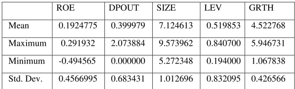
Table 2. Descriptive Statistics of the Dependent, Independent, and Control Variables
ROE DPOUT SIZE LEV GRTH
Mean 0.1924775 0.399979 7.124613 0.519853 4.522768 Maximum 0.291932 2.073884 9.573962 0.840700 5.946731 Minimum -0.494565 0.000000 5.272348 0.194000 1.067838 Std. Dev. 0.4566995 0.683431 1.012696 0.832095 0.426566
Source: Authors’ own calculation from annual reports of listed Agriculture firms
The table shows an average ROE of 19.24% for Ghanaian listed agriculture firms with a minimum and maximum returns of -49.5% and 29.2% respectively. This means that on average, stockholders receive Ghc0.19 of every Ghc1 invested annually. Some investors make profit while others incur losses on their investment. Firm size (SIZE) measures the spatial dimensions, proportions, and the magnitude of the firm.
Growth (GRTH) has been measured in relation to Amidu 2007, as the percentage increase in sales revenue over the previous year. The table shows that the listed agriculture companies were able to record a significant increase of 5.9 in revenue while observing a gradual movement in sales revenue of 1.1. On average, the agriculture firms recorded a substantial increase of 4.5 over the previous year. Leverage (LEV) measures the proportion of debt in the overall capital structure. This has been measured as the ratio of total liabilities to total assets of the company. From the table, the selected agriculture companies could be said to be less leveraged for a successful investment. However, a maximum and minimum of 84.1% and 19.4% were recorded respectively. This implies that agriculture firms are highly geared, and this makes it riskier for safe investments. On average, the firm is leveraged at 52%.
Discussion of Regression Results
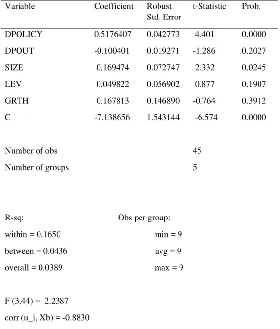
Table 3 reports regression results between the dependent variable and explanatory variables. An adjusted R square of 81.1% indicates that the model is strong fit and the variations in the dependent variable (ROE) can uniquely or jointly be explained by the independent variables (Pallant, 2007). The F-statistic (60.13) at p-value of 0.0000 explains the overall significance of the model. This indicates that there is a significance relationship between
Table 3. Summary of Regression Result of the model of the study
Variable Coefficient Robust Std. Error t-Statistic Prob. DPOLICY 0.5176407 0.042773 4.401 0.0000 DPOUT -0.100401 0.019271 -1.286 0.2027 SIZE 0.169474 0.072747 2.332 0.0245 LEV 0.049822 0.056902 0.877 0.1907 GRTH 0.167813 0.146890 -0.764 0.3912 C -7.138656 1.543144 -6.574 0.0000 Number of obs 45 Number of groups 5
R-sq: Obs per group:
within = 0.1650 min = 9 between = 0.0436 avg = 9 overall = 0.0389 max = 9 F (3,44) = 2.2387 corr (u_i, Xb) = -0.8830 Prob > F = 0.0003
Source: Authors’ own calculation from annual reports of listed firms
The results portray a positive and statistically significant relationship between Return on Equity (ROE) and dividend policy (DPOLICY). When dividend policy (DPOLICY) increases by 1% Return on Equity (ROE) increase by 51.56%. This implies that when a firm has a policy to pay dividend it influences its performance or profitability, and this may be a sign of good corporate governance system in place. This finding is consistent with empirical evidence of (Ross, et al 2002; Azam & Abbasi, 2011; Bremberger et. al, 2016). The results indicate a statistically insignificant and negative relationship between Return on Equity (ROE) and dividend payout (DPOUT). The negative coefficient means that if a firm pays more dividends relative to earnings, its performance deflates. High dividend payout agriculture firms in Ghana end up with low retained earnings for financing capital projects. Such agriculture firms may lack the financial capability to raise funds internally and may rely on debt financing to fund capital projects. The finding is congruent with the results of Amidu, (2007), Grullon et al., (2005)
and Farsio et al., (2004). However, it disaffirms the findings of Amidu (2007), Agyei and Marfo-Yiadom, (2011), and Adu-Boanyah et al., (2013).
Also, the results show that the coefficient of firm size and leverage are positive and statistically significant at 5%. A percentage increase of a firms’ size increases ROE by 16.95%. The results seem to suggest that, for listed Agriculture firms on GSE, leverage does not necessarily influence their return on equity. The positive association of a firm's size and return on equity indicates that increasing size is associated with an increase in performance (profitability). Growth (GRTH) in sales reports an insignificant positive relationship between ROE and growth. It reports a coefficient of (0.167813) from the regression table above. This indicates that as firms increase its sales revenue by 1%, the return of equity is more likely to increase. This is indicative of the fact that growing firms have a prospect of generating more returns for their owners. This is also consistent with studies by Marfo (2010) and Odalo et. al (2016). 4. Conclusion and Recommendation
The objective of the study was to establish the effect of dividend policy on the financial performance of listed Agriculture firms in Ghana. Dividend policy, dividend pay-out, firm size, leverage, growth were the independent variables and the dependent variable, return on equity. The results of the study revealed that dividend pay-out had no effect on the financial performance of listed Agriculture firms in Ghana. Thus, the number of dividends paid does not affect the financial performance of Agriculture firms but should pay dividends when they are financially strong. These findings were consistent with the research finding of Oppong (2015) which found that dividend policy does not affect companies' return on equity.
The findings of the study confirmed that dividend policy is a major factor that influences the financial performance of Agriculture firms. It was observed that dividend policy was a highly significant predictor in explaining the Agriculture firms' performance (ROE). Other factors such as firm size, leverage, and growth had an insignificant impact on the return of equity of listed Agriculture firms. Hence, agriculture firms should ensure that they have good and effective strategies that will lead to increased total assets and other factors that will result in the improved financial performance of banks and non-banking firms in the future.
The results of the study have these recommended policy implications. As dividend pay-out is still an important determinant of financial performance, management should, therefore, be mindful of the dividend policy decisions taken. Optimal dividend policy will better the lots of shareholders both in the short-run and long-run and more attract investors.
Also, agriculture firms should invest in profitable assets that will yield higher returns in the future to enhance their financial performance and attract investments in the future. Again, the research findings revealed that there was no weighty impact of dividend pay-out on the financial performance and hence, investors should not rely on the amount of dividend paid to ascertain the financial stability of firms.
References
Adu-Boanyah, E., Ayentimi, D. and Osei-Yaw, F. (2013), “Determinants of dividend payout policy of some selected Manufacturing firms listed on the Ghana Stock Exchange”, Research Journal of Finance and Accounting, vol. 4, no. 5, pp. 20-29. ISSN 2222-1697, E-ISSN 2222-2847
Agyei, S. K. and Marfo-Yiadom, E. (2011), “Dividend Policy and Bank Performance in Ghana”, International Journal of Economics and Finance, vol. 3, no. 4, pp. 20-31. DOI 10.5539/ijef.v3n4p202, ISSN 1916-971X, E-ISSN 1916-9728
Amidu, M. (2007) “How does dividend policy affect performance of the firm on Ghana stock Exchange”, Investment Management and Financial Innovations, vol. 4, no. 2, pp. 104 – 112, ISSN 1812-9358
Azam, M., Usmani, S. and Abassi, Z. (2011), “The impact of corporate governance on firm’s performance: Evidence from Oil and Gas Sector of Pakistan”, Australian Journal of basic and applied science, vol. 5, no. 12, pp. 2978 - 2983. [Online], Available: http://ajbasweb.com/old/ajbas/2011/December-2011/2978-2983.pdf, [Accessed: 25 Feb, 2020], ISSN 1991-8178
Bremberger, F., Cambini, C., Gugler, K. and Rondi, L. (2016). “Dividend policy in regulated network industries: Evidence from the EU”, Economic Inquiry, vol. 54, no. 1, pp. 408 - 432. E-ISSN 1465-7295, DOI 10.1111/ecin.12238.
Farsio, F., Geary, A. and Moser, J. (2004), “The relationship between dividends and earnings”, Journal for Economic Educators, vol. 4, no. 4, pp. 1 - 5. ISSN 0022-0485
Grullon, G., Michaely, R., Benartzi, S., and Thaler, R. H. (2005), “Dividend changes do not signal changes in future profitability”, The Journal of Business, vol. 78, no. 5, pp. 1659 - 1682. ISSN 0021-9398,DOI 10.1086/431438
Marfo, Y. (2010), “Dividend policy and the performance of banks in Ghana”, Journal of Economics and Accounting, vol. 10, no. 4, pp. 23 – 35, ISSN 0165-4101, DOI 10.22004/ag.econ.97084
Mashayekhi, B. and Bazazb, M. S. (2008), “Corporate governance and firm performance in Iran”, Journal of Contemporary Accounting & Economics, vol. 4, no. 2, pp. 156 - 172. ISSN 1815-5669, DOI 10.1016/S1815-5669(10)70033-3
Odalo, S. K., George, A. and Njuguna, A. G. (2016), “Relating Company Size and Financial Performance in Agricultural Firms Listed in the Nairobi Securities Exchange”, United States University of Africa Digital Resipotry, vol. 2, no. 4, pp. 6-15, ISSN 1916-971X, E-ISSN 1916-9728, DOI 10.5539/ijef.v8n9p34
Oppong, K. (2015), “Dividend policy and firms’ performance: a case of listed”, Doctoral Dissertation, Kwame Nkrumah University of Science and Technology, Kumasi- Ghana, [Online], Available: http://dspace.knust.edu.gh/handle/123456789/8651, [Accessed: 25 Feb, 2020], ISSN 1991-8178
Pallant, J. F. and Tennant, A. (2007), “An introduction to the Rasch measurement model: an example using the Hospital Anxiety and Depression Scale (HADS)”, British Journal of Clinical Psychology, vol. 46, no. 1, pp.1 - 18. 0144-6657, DOI 10.1348/014466506X96931 Shisia, A., Sang, W., Sirma, K. and Maundu, C. N. (2014), “Assessment of Dividend Policy on Financial Performance of Telecommunication Companies Quoted At the Nairobi Securities
Exchange”, International Journal of Economics, Commerce and Management, vol. 2, no. 10, pp. 1 - 21. ISSN 2348-0386, [Online], Available: http://ir.mksu.ac.ke/handle/123456780/4204, [Accessed: 28 Feb, 2020], ISSN 1991-8178
Wahla, K.-U.-R., Shah, S. Z. A. and Hussain, Z. (2012), “Impact of ownership structure on firm performance evidence from non-financial listed companies at Karachi Stock Exchange”, International Research Journal of Finance and Economics, vol. 84, pp. 6 - 13. ISSN 1450 2887, DOI 10.5296/ajfa.v6i1.4761