Piezoelectric-piezomagnetic behaviour of coated long fiber composites accounting for eigenfields

Science Arts & Métiers (SAM)

is an open access repository that collects the work of Arts et Métiers Institute of Technology researchers and makes it freely available over the web where possible.

This is an author-deposited version published in: https://sam.ensam.eu Handle ID: .http://hdl.handle.net/10985/16715

To cite this version :

George CHATZIGEORGIOU, Adil BENAARBIA, Fodil MERAGHNI - Piezoelectric-piezomagnetic behaviour of coated long fiber composites accounting for eigenfields Mechanics of Materials -Vol. 138, p.103157 - 2019

Piezoelectric-piezomagnetic behaviour of coated long fiber composites accounting for eigenfields

Journal Pre-proof

Piezoelectric-piezomagnetic behaviour of coated long fiber composites accounting for eigenfields

George Chatzigeorgiou, Adil Benaarbia, Fodil Meraghni

PII: S0167-6636(19)30550-2

DOI: https://doi.org/10.1016/j.mechmat.2019.103157

Reference: MECMAT 103157

To appear in: Mechanics of Materials

Received date: 28 June 2019

Revised date: 26 August 2019

Accepted date: 27 August 2019

Please cite this article as: George Chatzigeorgiou, Adil Benaarbia, Fodil Meraghni, Piezoelectric-piezomagnetic behaviour of coated long fiber composites accounting for eigenfields, Mechanics of Materials (2019), doi:https://doi.org/10.1016/j.mechmat.2019.103157

This is a PDF file of an article that has undergone enhancements after acceptance, such as the addition of a cover page and metadata, and formatting for readability, but it is not yet the definitive version of record. This version will undergo additional copyediting, typesetting and review before it is published in its final form, but we are providing this version to give early visibility of the article. Please note that, during the production process, errors may be discovered which could affect the content, and all legal disclaimers that apply to the journal pertain.

Highlights

• Micromechanical approach to evaluate the electro-magneto-inelastic properties in coated long fiber composites with transversely isotropic piezoelectric-piezomagnetic behaviour • Composite Cylinders Assemblage type of boundary conditions to obtain analytical

expres-sions of the dilute electro-magneto-mechanical concentration tensors

• Mori-Tanaka is adapted to identify i) the overall response of the composite, and ii) the various average electro-magneto-mechanical fields of the phases

• Ability of the proposed model to predict both macroscopic and average microscopic fields per phase when nonlinear fields take place

Piezoelectric-piezomagnetic behaviour of coated long fiber

composites accounting for eigenfields

George Chatzigeorgioua,˚_{, Adil Benaarbia}a_{, Fodil Meraghni}a

a_{Arts et M´etiers ParisTech, CNRS, Universit´e de Lorraine, LEM3, F-57000, Metz, France}

Abstract

A unified micromechanical approach is proposed to evaluate the electro-magneto-mechanical re-sponse of coated long fiber composites with transversely isotropic piezoelectric-piezomagnetic be-haviour. The developed framework takes into account the presence of electro-magneto-mechanical eigenfields. The multiscale strategy is based on solving specific boundary value problems in the same spirit as in the Composite Cylinders Assemblage technique. The solution of these prob-lems provides analytical expressions of the dilute electro-magneto-mechanical concentration ten-sors. With the help of the latter, the mean-field approach of Mori-Tanaka is adapted to identify i) the overall response of the composite, and ii) the various average electro-magneto-mechanical fields generated in the matrix, the fiber and the coating layers for known macroscopic fields. It is found that the novel approach has the same accuracy as existing homogenization techniques in terms of electro-magneto-mechanical properties. The ability of the proposed model to predict both macroscopic and average microscopic fields per phase when eigenfields take place is finally demonstrated.

Keywords: Composite Cylinders Assemblage; Coated long fiber composites; Piezoelectric-piezomagnetic materials, Electro-magneto-inelastic fields;

1. Introduction

Piezoelectric and piezomagnetic materials have received much attention in the last decades and are being increasingly used in various applications such as aerospace, biomedical, vibration

˚_{Corresponding author.}

Email addresses: georges.chatzigeorgiou@ensam.eu (George Chatzigeorgiou),

control and many others. These materials are extensively used as actuators, sensors and trans-ducers. Typically, active actuator materials have the capability to convert electrical and/or mag-netic energy into mechanical energy, while sensor materials provide an opposite conversion. To avoid the increased weight of conventional piezoelectric or piezomagnetic materials, these smart materials are generally combined with polymers in the form of composites. Such combination permits to develop new transducers and sensors with high strength, increased thermal conductiv-ity, low thermal expansion and advanced electromechanical behaviour. However, the co-existence of piezoelectic and piezomagnetic coupling effects in such composite materials and the involve-ment of many constituents-based parameters make the modelling of their multiphysical behaviour complex. From a micromechanics point of view, special techniques are required to investigate the coupling effects and the whole performance of the composite. Such modelling tools hold the key for using these smart composites in many applications in more intelligent ways.

The modelling of the piezoelectric-piezomagnetic composites is still an open topic (e.g., Nan, 1994; Wu and Huang, 2000; Bishay and Atluri, 2016; Ye et al., 2018; Kuo and Hsin, 2018, etc.). Within the last 30 years, significant progress has been made in the development of models that study the combined thermo-electro-magneto-elastic behaviour of composites (Tang and Yu, 2009; Bravo-Castillero et al., 2009; Akbarzadeh and Chen, 2014; Koutsawa, 2015). Most of the exist-ing models in literature were focused on the thermoelastic regime and have paid particular at-tention to the study of both piezoelectric and piezomagnetic coupling effects. Dunn and Taya (1993) have developed an Eshelby-type approach to investigate the electroelastic behaviour of piezoelectric composite materials by identifying appropriate Eshelby and concentration tensors. This approach has then been extended to consider electro-magneto-elastic responses (Huang and Kuo, 1997; Li and Dunn, 1998; Li, 2000). Huang et al. (1998) have identified electro-magneto-elastic Eshelby tensors for elliptical, rod, penny and ribbon shaped inclusions. Benveniste (1995) has studied the electro-magnetic effect in fibrous composites with piezoelectric and piezomag-netic phases using the composite cylinders assemblage method. Aboudi (2001) has developed a homogenization micromechanical method for the prediction of the effective moduli of coupled electro-magneto-thermo-elastic composites, while Lee et al. (2005) have proposed numerical and Eshelby-based analytical strategies for three phase electro-magneto-elastic composites. Moreover,

the electro-magneto-thermo-elastic composites have extensively been studied using the periodic homogenization theory (Bravo-Castillero et al., 2008, 2009; Challagulla and Georgiades, 2011; Hadjiloizi et al., 2013; Kuo and Peng, 2013). Pakam and Arockiarajan (2014) have developed a micromechanical scheme for studying ferroelectric and magnetostrictive composites reinforced with square cross section fibers and subjected to high electro-magnetic loading conditions. Using Hill’s interfacial operators, Dinzart and Sabar (2011) and Koutsawa et al. (2011) have proposed micromechanical models based on Mori-Tanaka and self consistent schemes to investigate the thermo-electro-magneto-elastic behaviour of magneto-piezoelectric composites with multi-coated ellipsoidal particles.

This work aims at developing a unified micromechanical approach in inelasticity to analytically express the electro-magneto-elastic and inelastic concentration tensors and effective material pa-rameters for coated long fiber composites with transversely isotropic piezoelectric-piezomagnetic behaviour. The coating between the matrix and the reinforcement is witnessing strong coupling effects with complex local behaviour. Inelastic deformation mechanisms such as plasticity and/or martensite transformation occur frequently at the coating region and strongly interact with the lo-cal damage of the matrix/reinforcement interface (Payandeh et al., 2010, 2012). To reiterate, one of the aims of this work is to develop appropriate tools to assess the electro-magneto-inelastic fields in the matrix, fibers and coating layers. The current work aims at elaborating multiscale approaches to design more accurate damage and failure criteria for piezoelectric-piezomagnetic composites.

A novel approach, adapted to the Mori-Tanaka homogenization scheme, is presented in this manuscript. The approach is based on solving specific boundary value problems, extending the composite cylinders model of Hashin and Rosen (1964) to account for the inelasticity. The latter effort can be considered as a generalization of the Dvorak and Benveniste (1992) methodology, providing analytical expressions of the dilute electro-magneto-mechanical concentration tensors, which can be utilized in classical micromechanical techniques, such as Mori-Tanaka or self con-sistent methods. The advantage of such information is that it permits to identify not only the overall response of the composite, but also the various average electro-magneto-mechanical fields generated in the matrix, the fiber and the coating layers for known macroscopic

mechanical conditions.

The effect of eigenfields (inelastic strains, electric or magnetic eigenfields) on the overall re-sponse, as well as in the average response of the phases, is important for the study of nonlinear behaviour of composites. Indeed, while in the current manuscript the described boundary value problems are linear, the provided solutions can be seen as the mean to include nonlinear mecha-nisms per phase. The latter should be described through evolution laws of the nonlinear fields and activation criteria. Via an appropriate incremental, iterative scheme, one can use the linearized mi-cromechanics solution provided here and adapt it to account for the constitutive laws of the phases (see for instance Pettermann et al., 1999 for purely mechanical multiscale analysis).

To fulfill the underlined objectives, a brief description of the Eshelby’s problem for coated in-homogeneity with eigenfields at the matrix fibers and coating layers is first presented. The Eshelby problem is then solved by considering special boundary condition problems analogue to those in-troduced by Hashin and Rosen. Then, numerical computations are conducted and discussed in detail. These computations have permitted to demonstrate the capabilities of the developed mi-cromechanics technique. Several conclusions, drawn from the findings, are finally put forward. 2. Preliminaries

For small deformations and rotations, electrostatic conditions with no electric charge and mag-netostatic conditions with no current density, the strain tensor, ε, the electric field vector, e, and the magnetic field vector, h, can be expressed with the help of the displacement vector, u, the elec-tric scalar potential, ae_{, and the magnetic scalar potential}1_{, a}m_{, respectively, through the tensorial}

relations

ε_“ 1

2 “

grad u ` rgrad usT‰_{, e“ ´grad a}e _{and h “ ´grad a}m_{, (1)}

1_{In classical magnetomechanics studies, the natural choice is to introduce a vector potential. When dealing with}

multiscale approaches, the absence of microscopic current density permits an alternative formalism with scalar poten-tial, which simplifies the calculations.

or the vector-type equations

ε _“ ” ε11 ε22 ε33 2ε12 2ε13 2ε23 ıT “ „ Bu1 Bx1 Bu2 Bx2 Bu3 Bx3 Bu1 Bx2 ` Bu2 Bx1 Bu1 Bx3 ` Bu3 Bx1 Bu2 Bx3 ` Bu3 Bx2 T , (2) e_“” e1 e2 e3 ıT “ „ ´Ba e Bx1 ´ Bae Bx2 ´ Bae Bx3 T , (3) h“” h1 h2 h3 ıT “ „ ´Bam Bx1 ´ Bam Bx2 ´ Bam Bx3 T , (4)

where the symbol r.sT _{stands for the usual vector/matrix transposes in orthogonal coordinates.}

On the other hand, the stress tensor, σ, the electric displacement, d, and the magnetic induc-tion, b, written in the vector-type forms

σ _“ ” σ11 σ22 σ33 σ12 σ13 σ23 ıT , d _“ ” d1 d2 d3 ıT , b_“” b1 b2 b3 ıT , (5)

obey the following equilibrium, electrostatic and magnetostatic equations

div σ “ 0, div d “ 0 and div b “ 0, (6)

or, in indicial form,

Bσ11{Bx1` Bσ12{Bx2` Bσ13{Bx3 “ 0,

Bσ12{Bx1` Bσ22{Bx2` Bσ23{Bx3 “ 0,

Bσ13{Bx1` Bσ23{Bx2` Bσ33{Bx3 “ 0,

Bd1{Bx1` Bd2{Bx2` Bd3{Bx3 “ 0,

Bb1{Bx1` Bb2{Bx2` Bb3{Bx3 “ 0. (7)

lowing constitutive laws, written in matrix-type notation2

σ_{“ L· rε ´ ε}p_{s ´ e· re ´ e}p_{s ´ f · rh ´ h}p_s, d“ eT·rε ´ εps ` κe·re ´ eps ` j· rh ´ hps,

b“ fT·rε ´ εps ` jT·re ´ eps ` κm·rh ´ hps, (8)

where the index p above a field denotes an eigenfield. Example of eigenfields are those

gener-ated by the presence of temperature (e.g. thermal expansion strain, etc.). In addition, L, κe_{, κ}m_,

e, f, j denote the elasticity, the dielectric properties, the magnetic permeabilities, the coupled

electro-mechanical, the coupled magneto-mechanical and the coupled electro-magnetic tensors, respectively. For transversely isotropic behaviour with axis of symmetry parallel to the direction 3, these tensors are expressed in the following matrix-type forms

L “ » — — — — — — — — — — — — — — — — — — — — — — — — – Ktr_{` µ</sub>tr <sub>K</sub>tr<sub>´ µ</sub>tr <sub>l 0 0 0</sub> Ktr<sub>´ µ</sub>tr <sub>K</sub>tr<sub>` µ}tr _{l 0 0 0} l l n 0 0 0 0 0 0 µtr _{0 0} 0 0 0 0 µax ₀ 0 0 0 0 0 µax fi ffi ffi ffi ffi ffi ffi ffi ffi ffi ffi ffi ffi ffi ffi ffi ffi ffi ffi ffi ffi ffi ffi ffi ffi fl , (9) e “ » — — — — — — — — — — — — – 0 0 e31 0 0 e31 0 0 e33 0 0 0 e15 0 0 0 e15 0 fi ffi ffi ffi ffi ffi ffi ffi ffi ffi ffi ffi ffi fl , f “ » — — — — — — — — — — — — – 0 0 f31 0 0 f31 0 0 f33 0 0 0 f15 0 0 0 f15 0 fi ffi ffi ffi ffi ffi ffi ffi ffi ffi ffi ffi ffi fl , (10)

2_{The symbol · in the matrix notation denotes the common matrix multiplication. The product between a scalar}

κe _“ » — — — – κe₁₁ 0 0 0 κe₁₁ 0 0 0 κe₃₃ fi ffi ffi ffi fl, κ m_“ » — — — – κ₁₁m 0 0 0 κm₁₁ 0 0 0 κm₃₃ fi ffi ffi ffi fl, (11) j “ » — — — – j11 0 0 0 j11 0 0 0 j33 fi ffi ffi ffi fl. (12) The constants Ktr_{, l, n, µ}tr_{, µ}ax_{, e}

31, e33, e15, f31, f33, f15, κe₁₁, κe₃₃, κ₁₁m, κm₃₃, j11 and j33 are material

parameters. Equation (8) can also be written in the following compact form

Σ“ L· rE ´ Eps , (13)

where L is the 12ˆ12 symmetric matrix given as L “ » — — — – L e f eT _´κe _{´ j} fT _{´ j}T _´κm fi ffi ffi ffi fl, (14)

and Σ, E, Ep_{the 12ˆ1 vectors defined as}

Σ“ ” σ d b ıT , E “” ε _{´e ´h} ıT , Ep “” εp _´ep _´hp ıT . (15)

Finally, the generalized vector

U “” u1 u2 u3 ae am

ıT

, (16)

is also introduced.

In the sequel, when dealing with various material phases, the following notation is postulated

for a quantity a: i) A superscript on the symbol of the form apqq _{denotes that the quantity a is}

spatially dependent. ii) A subscript on the symbol of the form aq is used for constant or average

value of the quantity. The index q can take the values 0, 1 or 2. 3. Coated long fiber composites with eigenfields

Identifying the overall properties of a composite sensitive to electro-magneto-mechanical load-ing conditions is the task of homogenization strategies and techniques. In this paper, the mean-field approach of the Mori-Tanaka method is followed. This method relies on two aspects:

• solving a basic (Eshelby-type) problem of a coated inhomogeneity embedded in an infinite medium, allowing to compute the so-called ”interaction” or ”dilute concentration” tensors. • using this information in the level of the composite for identifying the ”concentration”

ten-sors, whose knowledge leads to link the microscopic and macroscopic fields in order to

obtain the macroscopic matrix L and the macroscopic eigenfield Epof the overall

compos-ite.

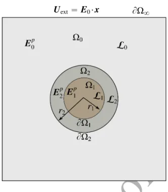
3.1. Eshelby’s problem for coated inhomogeneity with eigenfields in all phases

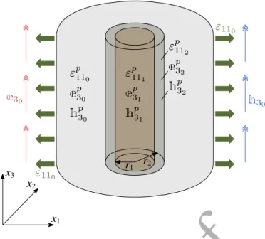
Consider a coated cylindrical inhomogeneity, embedded in an infinite medium. The medium, the inhomogeneity and the homothetic coated layer are characterized by constant generalized

mod-uli, L0, L1 and L2, respectively. The inhomogeneity occupies the space Ω1 with volume V1, is

bounded by the surface BΩ1 and is subjected to the uniform eigenfield E₁p. The coating layer

oc-cupies the space Ω2 with volume V2, is bounded by the surfaces BΩ1 and BΩ2 and is subjected

to the uniform eigenfield E₂p. The medium occupies the space Ω0, which is extended to infinity

(boundary surface BΩ8), and is subjected to the uniform eigenstrain E0p. At far distance, a linear

field Uext “ » — — — — — — — — — – u01 u02 u03 ae₀ am₀ fi ffi ffi ffi ffi ffi ffi ffi ffi ffi fl “ » — — — — — — — — — – ε110x1` ε120x2` ε130x3 ε120x1` ε220x2` ε230x3 ε130x1` ε230x2` ε330x3 ´e10x1´ e20x2´ e30x3 ´h10x1´ h20x2´ h30x3 fi ffi ffi ffi ffi ffi ffi ffi ffi ffi fl , (17)

with εi j0, ei0, hi0 (i, j “ 1, 2, 3) constant values, is applied (see Figure 1).

For this problem, which is a generalized version of the famous Eshelby inhomogeneity problem (Eshelby, 1957) accounting for multiphysics phenomena, the constitutive law is position depen-dent and reads

Σpxq “ $ ’ ’ ’ ’ ’ ’ & ’ ’ ’ ’ ’ ’ % L0·“Epxq ´ E₀p‰, x P Ω0, L1·“Epxq ´ E₁p‰, x P Ω1, L2·“Epxq ´ E₂p‰, x P Ω2. (18)

Figure 1: Cross section of coated cylindrical fiber with homothetic topology inside an infinite medium. All phases have homogeneous material properties and are subjected to uniform eigenfields. Moreover, the medium is subjected to linear displacement, electric potential and magnetic potential at far distance.

The boundary conditions correspond to uniform E0at far distance.

The main goal of this problem is to compute the average fields inside the inhomogeneity and inside the coating layer

E1 “ 1 V1 ż Ω1 Epxqdx and E2 “ 1 V2 ż Ω2 Epxqdx, (19)

respectively, when the applied field, E0, at far distance and the eigenfields E₀p, E₁p, E₂p are known.

In other words, the purpose is to evaluate the generalized, 12ˆ12 elastic and inelastic interaction tensors, Ti and Tp_q,ifor i “ 1, 2 and q “ 0, 1, 2, for which the following relations hold

Ei “ Ti· E0` 2 ÿ q_“0 Tp q,i· Eqp. (20)

The above expression is a direct extension of the corresponding one in the original Transformation Field Analysis approach of Dvorak and Benveniste (1992). In purely mechanical problems, the first term is the usual elastic interaction tensor of a phase, connecting the total strain in the phase

total strain in the phase i from the inelastic strains of all the phases in the representative volume element.

To assist the computations, the ratio φ “ V1{ rV1` V2s is identified.

3.2. Proposed methodology: analytical solutions in special boundary value problems

The proposed methodology is motivated by the studied boundary value problems by Hashin and Rosen (1964) in their famous composite cylinders assemblage theory. The necessary modifi-cations on these problems, discussed in the sequel, provide the exact solution for the interaction tensors. Similar technique has been utilized in various articles (Benveniste et al., 1989; Chatzige-orgiou et al., 2012; Wang et al., 2016; ChatzigeChatzige-orgiou and Meraghni, 2019; ChatzigeChatzige-orgiou et al., 2019) for studying the mechanical and piezoelectric response of long fiber composites.

Before passing to the actual boundary value problems, it is essential to express all the fields and the conservation laws in cylindrical coordinates.

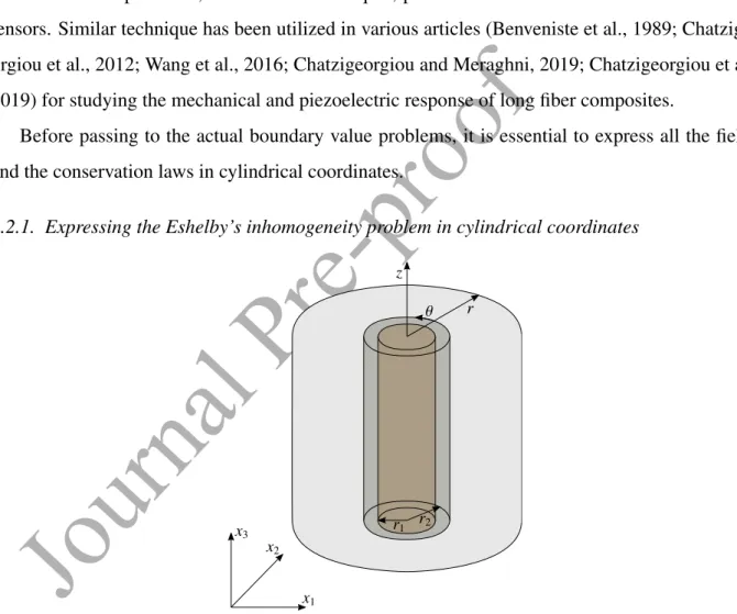
3.2.1. Expressing the Eshelby’s inhomogeneity problem in cylindrical coordinates

Figure 2: Coated cylindrical fiber with homothetic topology inside an infinite medium, which is represented as a concentric cylinder. All the fields are expressed in cylindrical coordinates.

Inside the representative volume element the various fields generated at every phase q (q “ 0, 1, 2) depend on the spatial position, i.e

Upqq_{pxq, E}pqq_{pxq, Σ}pqq_{pxq, E}ppqq_{pxq, @x P Ω}

q.

Due to the geometry of the inhomogeneities, the problem can be transformed in cylindrical co-ordinates, using a system of concentric cylinders for the inhomogeneity, the coating layer and the infinite matrix (see Figure 2). In cylindrical coordinates, the axes px, y, zq are transformed to pr, θ, zq, according to the relations

x1 “ r cos θ, x2 “ r sin θ, x3 “ z.

The vectors and tensors in cylindrical coordinates are noted with an arc above the symbol. Thus, in cylindrical coordinates, the fields are written as

(

Upqq_{pr, θ, zq,} E( pqq_{pr, θ, zq,} Σ( pqqpr, θ, zq,

(

Eppqq_{pr, θ, zq, @r, θ, z P Ω}q,

while the equilibrium, electrostatic and magnetostatic equations are re-expressed as Bσ( pqq_rr Br ` 1 r Bσ( pqq<sub>rθ</sub> Bθ ` ( σpqq_{rr ´}σ( pqq_θθ r ` Bσ( pqq<sub>rz</sub> Bz “ 0, Bσ( pqq<sub>rθ</sub> Br ` 1 r Bσ( pqq_θθ Bθ ` 2σ( pqq<sub>rθ</sub> r ` Bσ( pqq_θz Bz “ 0, Bσ( pqq_rz Br ` 1 r Bσ( pqq<sub>θz</sub> Bθ ` ( σpqq_rz r ` Bσ( pqq<sub>zz</sub> Bz “ 0, B ( dpqq<sub>r</sub> Br ` 1 r B ( dpqq_θ Bθ ` ( dpqq<sub>r</sub> r ` B ( dpqq_z Bz “ 0, B ( bpqq_r Br ` 1 r B ( bpqq<sub>θ</sub> Bθ ` ( bpqq_r r ` B ( bpqq_z Bz “ 0. (21)

In addition, the strain, electric and magnetic field components in each phase are given using the following expressions ( εpqq _“ ” ε( pqq_rr ε( pqq_θθ ε( pqq_zz 2ε(pqq_rθ 2ε(pqq_rz 2ε(pqq_θz ıT “ « Bu(pqq_r Br 1 r Bu( pqq_θ Bθ ` ( upqq<sub>r</sub> r Bu(pqq<sub>z</sub> Bz Bu(pqq<sub>θ</sub> Br ` 1 r Bu( pqq_r Bθ ´ ( upqq_θ r Bu( pqq_z Br ` Bu( pqq<sub>r</sub> Bz 1 r Bu( pqq<sub>z</sub> Bθ ` Bu( pqq_θ Bz ffT , (22)

( epqq“” e( pqq_r e( pqq_θ e( pqq_z ıT “ „ ´Baepqq Br ´ 1 r Baepqq Bθ ´ Baepqq Bz T , (23) ( hpqq_“” ( hpqq_r ( hpqq_θ ( hpqq_z ıT “ „ ´Bampqq Br ´ 1 r Bampqq Bθ ´ Bampqq Bz T . (24)

The inhomogeneity is considered to have radius r equal to r1 and the coating layer has external

radius r2(see Figure 1). Using the radii of the concentric cylinders, one obtains φ “ r₁2{r₂2.

The continuity conditions between i) the inhomogeneity and the coating layer, and ii) the coating and the matrix are expressed through the relations

( up1q_{s pr}1, θ,zq “ ( up2q_{s pr}1, θ,zq, s “ r, θ or z, ( up2q_{s pr}2, θ,zq “ ( up0q_{s pr}2, θ,zq, s “ r, θ or z, asp1q_pr1, θ,zq “ asp2qpr1, θ,zq, s “ e or m, asp2q_pr2, θ,zq “ asp0qpr2, θ,zq, s “ e or m, (25) and ( σp1q_{S pr}1, θ,zq “ ( σp2q_{S pr}1, θ,zq, S “ rr, rθ or rz, ( σp2q_{S pr}2, θ,zq “ ( σp0q_{S pr}2, θ,zq, S “ rr, rθ or rz, ( dp1q_{r pr}1, θ,zq “ ( dp2q_{r pr}1, θ,zq, ( dp2q_{r pr}2, θ,zq “ ( dp0q_{r pr}2, θ,zq, ( bp1q_{r pr}1, θ,zq “ ( bp2q_{r pr}1, θ,zq, ( bp2q_{r pr}2, θ,zq “ ( bp0q_{r pr}2, θ,zq. (26)

Due to the transverse isotropy of all phases, the generalized modulus, L, retains the same form in cylindrical coordinates.

In the following subsections, the boundary value problems are presented and the analytical form of the solution (in terms of the generalized vector

(

Upqq) is given. 3.2.2. Analytical boundary value problems

The four boundary value problems which allow to compute the interaction tensors are the following:

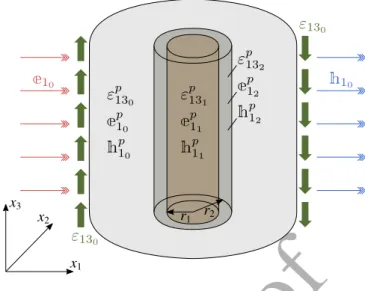
• Axial shear / in-plane electric and magnetic field

ε130 ε130 e1 0 h10 h εp₁₃₀ e p 10 h p 10 e h εp₁₃₁ e p 11 h p 11 e h εp₁₃₂ e p 12 h p 12 e h

Figure 3: Boundary value problem for axial shear / in-plane electric and magnetic field conditions.

Displacement, electric and magnetic potential boundary conditions at far field (when rext

tends to infinity) are expressed using the following formulas

(

u_rext “ u(_θext “ 0,

(

u_zext “ βrextcos θ,

aeext “ ´βerextcos θ,

amext “ ´βmrextcos θ, (27)

where β, βe _{and β}m _{are considered known. In addition, all phases are subjected to the}

fol-lowing eigenfields ( εppqq _{“ s}q ” 0 0 0 0 cos θ ´ sin θ ıT, ( eppqq “ seq ” cos θ ´ sin θ 0 ıT, ( hppqq “ smq ” cos θ ´ sin θ 0 ıT, (28)

for q “ 0, 1, 2 and the values of sq, seqand smq being known. The latter expressions correspond

x1 direction (see Figure 3). The analytical solution for the displacement field, the electric

potential and the magnetic potential at every r, θ and z takes the form

( upqq_r “ u( pqq_θ “ 0, ( upqq_{z “ r} 2 ÿ i“1 Ξq,i „ r r1 ξi´1 cos θ, aepqq _{“ ´r} 2 ÿ i“1 Ξe_q,i „ r r1 ξi´1 cos θ, ampqq _{“ ´r} 2 ÿ i“1 Ξm_q,i „ r r1 ξi´1 cos θ, (29)

with ξ1 “ 1 and ξ2 “ ´1. The unknown coefficients Ξq,i, Ξe_q,i and Ξm_q,i are determined

from the boundary conditions, the interface relations (25), (26) and the condition that the displacements, the magnetic potential and the electric potential are finite at r “ 0.

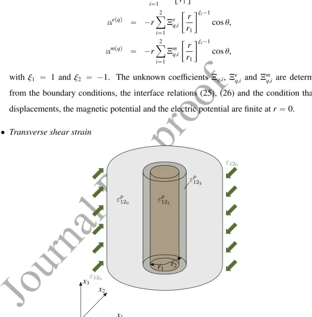
• Transverse shear strain e h e h ε120 ε120 e h e h εp₁₂₀ e h e h ε p 121 e h e h εp₁₂ 2

Figure 4: Boundary value problem for transverse shear strain conditions.

using the following equations

(

u_{rext “ γr}extsin 2θ,

(

u_{θext “ γr}extcos 2θ,

(

u_{zext “ 0,} (30)

where γ is known. All phases are also subjected to the eigenstrains

( εppqq _{“ 2s}q „ 1 2sin 2θ ´ 1 2sin 2θ 0 cos 2θ 0 0 T , (31)

for q “ 0, 1, 2 and the value of sqbeing known. The latter expression corresponds to uniform

shear strain on the plane x1´ x2(see Figure 4). The analytical solution for the displacement

field at every r, θ and z takes the following form

( upqq_r “ r 4 ÿ i“1 Ξq,iψq,i „_r r1 ξi´1 sin 2θ, ( upqq_θ “ r 4 ÿ i“1 Ξq,i „ r r1 ξi´1 cos 2θ, ( upqq_{z “ 0,} (32) with ξ1“ 3, ψq,1 “ Kq´ µq 2Kq` µq, ξ2“ 1, ψq,2 “ 1, ξ3 “ ´3, ψq,3 “ ´1, ξ4 “ ´1, ψq,4 “ Kq` µq µq . (33)

In such loading case, the unknown coefficients Ξq,i are determined from the boundary

con-ditions, the interface relations (25), (26) and the condition that the displacements are finite at r “ 0.

h ε110 ε110 e3 0 h3 0 e h εp₁₁₀ e p 30 h p 30 e h εp₁₁₁ e p 31 h p 31 e h εp₁₁₂ e p 32 h p 32

Figure 5: Boundary value plane strain / axial electric and magnetic field conditions. Case of uniaxial strain in the x1

direction.

Displacement, electric and magnetic potential boundary conditions at far field (when rext

tends to infinity) are expressed as follows

(

u_{rext “ βr}ext` γrextcos 2θ,

(

u_{θext “ ´γr}extsin 2θ,

(

u_{zext “ 0,} aeext “ ´βez,

amext “ ´βmz, (34)

where β, γ, βe _{and β}m_{are assumed known. All phases are subjected to the eigenfields}

( εppqq _{“ s}q,β ” 1 1 0 0 0 0 ıT `2sq,γ „ 1 2cos 2θ ´ 1 2cos 2θ 0 ´ sin 2θ 0 0 T , ( eppqq “ seq ” 0 0 1 ıT, ( hppqq “ smq ” 0 0 1 ıT, (35)

correspond to uniform biaxial strain state with normal components on the x1 and x2

direc-tions, and uniform electric and magnetic fields in the x3 direction. Two special cases are

considered here:

– uniform strain at the x1 direction, which is obtained by setting γ “ β and sq,γ “ sq,β

(see Figure 5),

– uniform strain at the x2direction, which is obtained by setting γ “ ´β and sq,γ “ ´sq,β.

The analytical solution for the displacement field, the electric potential and the magnetic potential at every r, θ and z takes the following form

( upqq_{r “ r} 4 ÿ i“1 Ξq,iψq,i „_r r1 ξi´1 cos 2θ ` r 2 ÿ i“1 Zq,i „_r r1 ζi´1 , ( upqq_θ “ ´r 4 ÿ i“1 Ξq,i „_r r1 ξi´1 sin 2θ, ( upqq_{z “ 0,} aepqq _{“ ´β}ez, ampqq _{“ ´β}mz. (36)

In the above expressions, ζ1 “ 1 and ζ2 “ ´1, while ψq,i and ξi for i “ 1, 2, 3, 4 are given

by the relations described in the previous boundary value problem. Moreover, the unknown

coefficients Ξq,i, Zq,i are determined from the boundary conditions, the interface relations

(25), (26) and the condition that the displacements are finite at r “ 0. • Hydrostatic strain / axial inelastic strain

Displacement boundary conditions at far field correspond to hydrostatic strain where

(

u_{rext “ βr}ext,

(

u_{θext “ 0 and} u(_{zext “ βz}ext. (37)

All phases are subjected to the eigenstrains

(

εppqq _{“ s}q

”

h ε110 ε110 e h ε220 ε220 ε330 “ ε110 ε330 “ ε110 “ “ e h e h εp₃₃₀ e h e h εp₃₃₁ e h e h εp₃₃ 2

Figure 6: Boundary value problem for hydrostatic strain / axial inelastic strain conditions.

for q “ 0, 1, 2 and the value of sqbeing known. The latter expression corresponds to uniform

inelastic strain in the x3direction (see Figure 6). The analytical solution for the displacement

field at every r, θ and z takes the following form

( upqq_{r “ r} 2 ÿ i“1 Zq,i „ r r1 ζi´1 , u( pqq_{θ “ 0 and} u( pqq_{z “ βz,} (39)

with ζ1 “ 1 and ζ2 “ ´1. The unknown coefficients Zq,i are determined from the boundary

conditions, the interface relations (25), (26) and the condition that the displacements are finite at r “ 0.

3.2.3. Computing the interaction tensors

Solving the previously described boundary value problems, the fieldsE( pqqcan be computed in

both the fiber and its coating. Consequently, the average values E1and E2, expressed in Cartesian

coordinates, can be evaluated analytically with the help of the expressions (19). In these studies, the values of β, γ, βe_{, β}m_{, s}

q, sq,β, sq,γ, seqand smq can be chosen properly in order to “construct” the

interaction tensors (for instance, setting one equal to 1 and zero to the rest). The four discussed

boundary value problems are sufficient for identifying all the terms of Ti and Tp_q,i. The

described in Chatzigeorgiou and Meraghni (2019); Chatzigeorgiou et al. (2019).

It is important to note that the general forms of the elastic and inelastic interaction tensors in all phases are given by the expressions

T “ » — — — — — — – T00 _T0e _T0m Te0 _Tee _Tem Tm0 _Tme _Tmm fi ffi ffi ffi ffi ffi ffi fl , Tp _“ » — — — — — — – Tp00 _Tp0e _Tp0m Tpe0 _Tpee _Tpem Tpm0 _Tpme _Tpmm fi ffi ffi ffi ffi ffi ffi fl , (40)

where the various submatrices are written as

T00_“ » — — — — — — — — — — — — — — — — — — — — — – 1 2 “ rTxxsmec` rTxysmec ‰ 1 2 “ rTxxsmec´ rTxysmec ‰ rTzzsmec´ rTxxsmec 0 0 0 1 2 “ rTxxsmec´ rTxysmec ‰ 1 2 “ rTxxsmec` rTxysmec ‰ rTzzsmec´ rTxxsmec 0 0 0 0 0 1 0 0 0 0 0 0 rTxysmec 0 0 0 0 0 0 rTxzsmec 0 0 0 0 0 0 rTxzsmec fi ffi ffi ffi ffi ffi ffi ffi ffi ffi ffi ffi ffi ffi ffi ffi ffi ffi ffi ffi ffi ffi fl , (41) Tp00_“ » — — — — — — — — — — — — — — — — — — — — — – 1 2 ” rTp xxsmec` “<sub>T</sub>p xy ‰ mec ı 1 2 ” rTp xxsmec´ “<sub>T</sub>p xy ‰ mec ı rTp zzsmec´ rTxxpsmec 0 0 0 1 2 ” rTp xxsmec´ “ Tp xy ‰ mec ı 1 2 ” rTp xxsmec` “ Tp xy ‰ mec ı rTzzpsmec´ rTxxpsmec 0 0 0 0 0 0 0 0 0 0 0 0 “Txyp‰_mec 0 0 0 0 0 0 rTp xzsmec 0 0 0 0 0 0 rTxzpsmec fi ffi ffi ffi ffi ffi ffi ffi ffi ffi ffi ffi ffi ffi ffi ffi ffi ffi ffi ffi ffi ffi fl , (42) Te0 “ » — — — — — — – 0 0 0 0 “Te xz ‰ mec 0 0 0 0 0 0 “Te xz ‰ mec 0 0 0 0 0 0 fi ffi ffi ffi ffi ffi ffi fl , (43)

Tpe0 “ » — — — — — — – 0 0 0 0 _rTxzpesmec 0 0 0 0 0 0 _rTxzpesmec 0 0 0 0 0 0 fi ffi ffi ffi ffi ffi ffi fl , (44) Tm0 _“ » — — — — — — – 0 0 0 0 “Tm xz ‰ mec 0 0 0 0 0 0 “Tm xz ‰ mec 0 0 0 0 0 0 fi ffi ffi ffi ffi ffi ffi fl , (45) Tpm0 _“ » — — — — — — – 0 0 0 0 _rTxzpmsmec 0 0 0 0 0 0 _rTxzpmsmec 0 0 0 0 0 0 fi ffi ffi ffi ffi ffi ffi fl , (46) T0e_“ » — — — — — — — — — — — — — — — — — — — — – 0 0 rTxxselc 0 0 rTxxselc 0 0 0 0 0 0 rTxzselc 0 0 0 rTxzselc 0 fi ffi ffi ffi ffi ffi ffi ffi ffi ffi ffi ffi ffi ffi ffi ffi ffi ffi ffi ffi ffi fl , Tp0e_“ » — — — — — — — — — — — — — — — — — — — — – 0 0 rTxxpselc 0 0 rTxxpselc 0 0 0 0 0 0 rTxzpselc 0 0 0 rTxzpselc 0 fi ffi ffi ffi ffi ffi ffi ffi ffi ffi ffi ffi ffi ffi ffi ffi ffi ffi ffi ffi ffi fl , (47)

T0m_“ » — — — — — — — — — — — — — — — — — — — — – 0 0 _rTxxsmag 0 0 _rTxxsmag 0 0 0 0 0 0 rTxzsmag 0 0 0 _rTxzsmag 0 fi ffi ffi ffi ffi ffi ffi ffi ffi ffi ffi ffi ffi ffi ffi ffi ffi ffi ffi ffi ffi fl , Tp0m_“ » — — — — — — — — — — — — — — — — — — — — – 0 0 _rTxxpsmag 0 0 _rTxxpsmag 0 0 0 0 0 0 rTp xzsmag 0 0 0 _rTp xzsmag 0 fi ffi ffi ffi ffi ffi ffi ffi ffi ffi ffi ffi ffi ffi ffi ffi ffi ffi ffi ffi ffi fl , (48) Tee _“ » — — — — — — – “ Te xz ‰ elc 0 0 0 “Te xz ‰ elc 0 0 0 1 fi ffi ffi ffi ffi ffi ffi fl , Tpee _“ » — — — — — — – rTxzpeselc 0 0 0 _rTxzpeselc 0 0 0 0 fi ffi ffi ffi ffi ffi ffi fl , (49) Tmm _“ » — — — — — — – “ Tm xz ‰ mag 0 0 0 “Tm xz ‰ mag 0 0 0 1 fi ffi ffi ffi ffi ffi ffi fl , Tpmm _“ » — — — — — — – rTxzpmsmag 0 0 0 _rTxzpmsmag 0 0 0 0 fi ffi ffi ffi ffi ffi ffi fl , (50) Tme_“ » — — — — — — – “ Tm xz ‰ elc 0 0 0 “Tm xz ‰ elc 0 0 0 0 fi ffi ffi ffi ffi ffi ffi fl , Tpme “ » — — — — — — – rTxzpmselc 0 0 0 _rTxzpmselc 0 0 0 0 fi ffi ffi ffi ffi ffi ffi fl , (51) Tem_“ » — — — — — — – “ Te xz ‰ mag 0 0 0 “Te xz ‰ mag 0 0 0 0 fi ffi ffi ffi ffi ffi ffi fl , Tpem _“ » — — — — — — – rTxzpesmag 0 0 0 _rTxzpesmag 0 0 0 0 fi ffi ffi ffi ffi ffi ffi fl . (52)

In the above formulas, the symbols rt‚usmec, rt‚uselc and rt‚usmag denote quantities that are

ac-tivated by the presence of strains, electric fields and magnetic fields, respectively. Appendix A presents the computational details for obtaining the various T terms.

3.3. Alternative approach: Hill’s interfacial operators

The solution to the original problem proposed by Eshelby (1957) is valid for uncoated inho-mogeneities of ellipsoidal shape inside a matrix material. In the case of coated inhomogeneity, the Eshelby approach provides information for the average strain inside the inhomogeneity/coating system. To identify the strains at each phase, one can use the concept of the interfacial operators (Walpole, 1978; Hill, 1983). This technique has been widely utilized in the literature for com-posites with mechanical (Cherkaoui et al., 1995; Berbenni and Cherkaoui, 2010; Chatzigeorgiou and Meraghni, 2019), piezoelectric (Chatzigeorgiou et al., 2019), thermo-piezoelectric (Koutsawa et al., 2010), piezoelectric-piezomagnetic (Dinzart and Sabar, 2011), and thermo-piezoelectric-piezomagnetic (Koutsawa et al., 2011) behaviour.

The computational steps for obtaining the elastic and interaction tensors for a composite with pure mechanical behaviour have been described in detail in Chatzigeorgiou and Meraghni (2019). For a piezoelectric-piezomagnetic composite the procedure is similar, with the only difference that the fields have the extended form presented in section 2. It is important to point out that the use of Hill’s interfacial operators implies implicitly the hypothesis that in the Eshelby problem the total fields inside the inhomogeneity are uniform. As has been illustrated in Chatzigeorgiou and Meraghni (2019), under transverse shear conditions this hypothesis is violated in long fiber composites and thus can provide inaccurate results in certain cases.

3.4. Mori-Tanaka approach

Once the tensors Tiand T_q,ip are identified with one of the two approaches discussed previously,

one can pass to the next step and consider the composite.

A direct approach, like for instance the generalized self consistent composite cylinders method (Christensen, 1979), is applicable for the problem under investigation. It provides the local distri-bution of the fields in the representative volume element, but it is quite limited, since it is designed exclusively for unidirectional fiber composites with random distribution of the fibers. The current work considers the Mori-Tanaka method for identifying the macroscopic response of the com-posite. A mean-field approach is more flexible in terms of microstructural characteristics; it can account for non-uniform distributions of the fibers, or the presence of different types of

ment. The restriction of the proposed methodology is that it estimates only average fields per material phase and not their actual spatial distribution, which is the case for full field approaches.

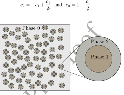
A unidirectional coated fiber composite consists of a matrix phase in which coated fibers are distributed randomly (see Figure 7). In this three-phase composite, the volume fractions of the

matrix, the fibers and their coating are denoted as cq, q “ 0, 1, 2. Using the ratio, φ, the following

relations can be given

c2 “ ´c1` c1 φ and c0 “ 1 ´ c1 φ. (53) h e h e h e h e h e h e h e h Phase 0 Phase 1 Phase 2

Figure 7: Cross section of unidirectional fiber composite. The fibers are coated and all phases exhibit piezoelectric-piezomagnetic behaviour.

According to the basic principle of all multiscale methods, the macroscopic fields at a macro-scopic point are equal to the average of the corresponding micromacro-scopic fields over the representa-tive volume element linked with the specific macroscopic point. In the composite considered here, the macroscopic fields, E and Σ, are given by

E “ c0E0` c1E1` c2E2,

Σ “ c0Σ0` c1Σ1` c2Σ2. (54)

Moreover, the constitutive law for each phase can be written in its average form

In the Mori-Tanaka method, the far field, E0, and the eigenfield, E₀p, of the expressions (20)

correspond to the average field and the average eigenfield of the matrix phase of the composite.

Combining (20) and (54)1, and after some algebra, the following relations are derived for r “

0, 1, 2 Er“ Ar· E ` 2 ÿ q“0 Ap q,r· Eqp, (56) with A0 “ « c0I ` 2 ÿ i“1 ciTi ff´1 , As “ Ts· A0, A_q,p_{0 “ ´A}0· 2 ÿ i“1 ciT_q,ip , Aq,sp “ Tpq,s´ As· 2 ÿ i“1 ciT_q,ip , (57)

for q “ 0, 1, 2 and s “ 1, 2. In the above expression, I is the 12ˆ12 identity matrix. Moreover,

combining equations (20), (56), (57) and (54)2, yields

Σ“ L·rE ´ Eps, (58) with L “ 2 ÿ i“0 ciLi· Ai, Ep “ 2 ÿ q“0 Ap q· Epq, Aqp “ L´1· « cqLq´ 2 ÿ i“0 ciLi· Aq,ip ff . (59)

It is worth noting that non-uniform distributions of fibers can be accounted for by introducing appropriate orientation distribution functions in the expressions (57) and (59). One should bear in mind that the Mori-Tanaka scheme for reinforced composites with non-uniform alignment may lead to non-symmetric macroscopic magneto-electro-mechanical matrix L. The symmetry issue could be potentially resolved by choosing another mean-field approach with similar structure, for example the Casta˜neda and Willis method (Ponte-Casta˜neda and Willis, 1995; Giordano, 2017). The latter assumes a unified ellipsoidal shape for the distribution of heterogeneities, which pro-vides a consistent homogenization scheme and ensures the symmetry of the macroscopic matrix L for non-uniform alignment of the fibers.

4. Numerical applications

The purpose of this section is to demonstrate the developed micromechanics technique

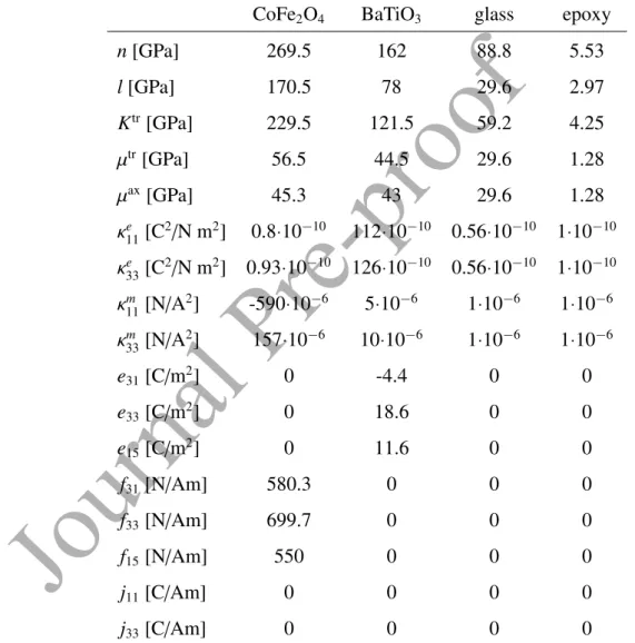
capa-bilities. For the needs of the numerical examples, four different materials are examined: CoFe2O4,

BaTiO3, glass and epoxy. The first one exhibits piezomagnetic behaviour, the second has

piezo-electric characteristics and the last two present a typical mechanical response without magnetome-chanical or electromemagnetome-chanical couplings. The material parameters of these materials are summa-rized in Table 1.

CoFe2O4 BaTiO3 glass epoxy

n[GPa] 269.5 162 88.8 5.53 l[GPa] 170.5 78 29.6 2.97 Ktr _{[GPa] 229.5 121.5 59.2 4.25} µtr[GPa] 56.5 44.5 29.6 1.28 µax[GPa] 45.3 43 29.6 1.28 κe₁₁[C2_{/N m}2_{] 0.8¨10}´10 _112¨10´10 _0.56¨10´10 _1¨10´10 κe₃₃[C2/N m2] 0.93¨10´10 126¨10´10 0.56¨10´10 1¨10´10 κm₁₁[N/A2_{] -590¨10}´6 _5¨10´6 _1¨10´6 _1¨10´6 κm₃₃[N/A2] 157¨10´6 10¨10´6 1¨10´6 1¨10´6 e31[C/m2] 0 -4.4 0 0 e33[C/m2] 0 18.6 0 0 e15[C/m2] 0 11.6 0 0 f31[N/Am] 580.3 0 0 0 f33[N/Am] 699.7 0 0 0 f15[N/Am] 550 0 0 0 j11[C/Am] 0 0 0 0 j33[C/Am] 0 0 0 0

Table 1: Electro-magneto-mechanical properties for the materials utilized in the numerical examples. The properties of CoFe2O4, BaTiO3and epoxy have been obtained from Lee et al. (2005). The material parameters for the glass have

4.1. Validation

In the first subsection, the electro-magneto-elastic properties of long fibers composites with and without coating layer are computed with the proposed method and are compared with the predictions of other methods in the literature.

Fiber volume fraction

0 0.2 0.4 0.6 0.8 1

Effective elastic moduli [Pa]

×1011 0 0.5 1 1.5 2 2.5 3 L11 L33 L12 L13 L55 d b b d

b Fiber volume fraction

0 0.2 0.4 0.6 0.8 1

Effective piezoelectic moduli [C/m

2] -5 0 5 10 15 20 e31 e33 e15 d b b d b (a) (b)

Fiber volume fraction

0 0.2 0.4 0.6 0.8 1

Effective magneto-electric modulus [C/m

2] _×10-9 0 0.5 1 1.5 2 2.5 3 j33 d b b d b (c)

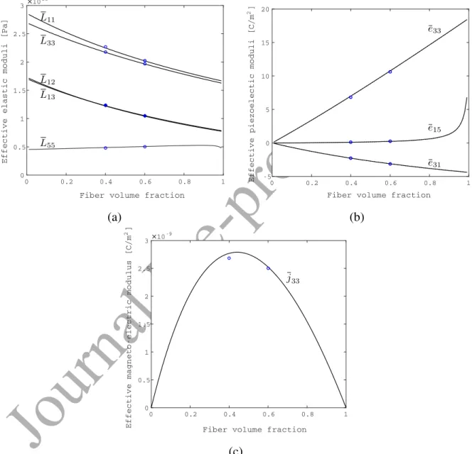
Figure 8: Material properties as a function of the fiber volume fraction for a composite consisting of CoFe2O4matrix

and BaTiO3 long fibers: (a) mechanical, (b) piezoelectric and (c) electromagnetic coefficients. Comparison of the

In the first example, a composite consisting of CoFe2O4 matrix and BaTiO3 long fibers is

analyzed and the results are compared with the periodic homogenization predictions provided by Lee et al. (2005). The mechanical stiffness coefficients, the piezoelectric coupling terms and the electromagnetic coupling terms are demonstrated in Figure 8 as a function of the fiber volume fraction. The numerical results for the periodic homogenization analyses have been obtained only for two different volume fractions, 40% and 60% percent. As it can be observed, the new model simulations are in excellent agreement with the full field homogenization results.

Coated fiber volume fraction

0 0.2 0.4 0.6 0.8 1

Effective magneto-electric modulus [C/m

2 ] ×10-12 0 0.5 1 1.5 j11[new approach] j11[DinSab] d b b d

b Coated fiber volume fraction

0 0.2 0.4 0.6 0.8 1

Effective magneto-electric modulus [C/m

2 ] ×10-10 0 0.5 1 1.5 2 2.5 3 3.5 4 j33[new approach] j33[DinSab] d b b d b (a) (b)

Figure 9: Electromagnetic properties as a function of the coated fiber volume fraction of a composite consisting of CoFe2O4matrix and glass fibers coated with BaTiO3coating layer: Comparison of the developed method predictions

(solid lines) with numerical results obtained by Dinzart and Sabar (2011) (points).

The second example illustrates results from studies in Dinzart and Sabar (2011). In that paper, an Eshelby-based micromechanics technique was developed using the Hill’s interfacial operators.

In their analysis, glass fibers coated with BaTiO3coating layer are embedded in CoFe2O4 matrix.

The aspect ratio of the fibers (length to radius diameter) is 100, which is quite large and can serve for the purpose of this paper as almost long fiber. The ratio φ for the coated fibers is taken equal to 82.645%. Figure 9 illustrates the electromagnetic coupling terms of the composite as a function of the fiber volume fraction. The results of both methods are in good agreement and the small

difference is mainly due to the finite value of the fibers’ aspect ratio.

The above preliminary examples demonstrate that the new approach has the same accuracy with existing homogenization techniques in terms of electro-magneto-mechanical properties. The following numerical studies demonstrate the ability of the model to predict both macroscopic and average microscopic fields per phase when nonlinear fields take place.

4.2. Applied thermal strains

A typical example of inelastic deformation is the appearance of thermal strains. Consider

a composite made of CoFe2O4 matrix and glass fibers coated with BaTiO3 coating layer. The

composite is assumed free from external loading and only a temperature difference of 1 K is applied. The thermal expansion coefficients for the matrix, the fiber and the coating are taken

equal to 10´5_{1/K, 5 ¨ 10}´6_{1/K and 6.4 ¨ 10}´6_{1/K respectively.}

According to the general principles of homogenization of composites subjected to thermome-chanical processes, the microscopic and macroscopic temperature coincide (Chatzigeorgiou et al., 2018), i.e. all material phases in the RVE are subjected to the same temperature difference of 1 K. This leads to the development of inelastic (thermal) strains in all phases:

ε₀p _“ ” 10´5 ₁₀´5 ₁₀´5 _{0 0 0} ıT_,

ε₁p _“ ” _{5 ¨ 10}´6 _{5 ¨ 10}´6 _{5 ¨ 10}´6 _{0 0 0} ıT_,

ε₂p _“ ” _{6.4 ¨ 10}´6 _{6.4 ¨ 10}´6 _{6.4 ¨ 10}´6 _{0 0 0} ıT_.

Figure 10 illustrates the non zero terms of the macroscopic stress tensor, the electric displace-ment vector and the magnetic induction vector that are generated due to the thermal strains as a function of the fiber volume fraction. Considering the coating, two different ratios φ are consid-ered: φ “ 50% and φ “ 80%. From these results one observes that the stresses and the magnetic

induction increase with the increase of c1, while the electric displacement initially has a small

Fiber volume fraction [%]

0 10 20 30 40 50 Macroscopic fields -7 -6 -5 -4 -3 -2 -1 0 1 σ11[MPa] σ22[MPa] σ33[MPa] d3[10´5C/m 2_] b3 [10´2N/Am] b d

b Fiber volume fraction [%]

0 20 40 60 80 Macroscopic fields -7 -6 -5 -4 -3 -2 -1 0 1 σ11[MPa] σ22[MPa] σ33[MPa] d3[10´5C/m 2_] b3[10´2N/Am] b d b (a) (b)

Figure 10: Composite consisting of CoFe2O4matrix and glass fibers coated with BaTiO3coating layer. Macroscopic

stress, electric displacement and magnetic induction fields, caused by thermal strains: (a) ratio φ_{“ 50% and (b) ratio} φ_{“ 80%.} 0.00 Microscopic fields (c1 “ 20%, φ “ 50%) σ11 [MPa] d3 [10 ´5 _C/m2_] b3 [10´2 N/Am] b d b

Figure 11: Composite consisting of CoFe2O4 matrix and glass fibers coated with BaTiO3 coating layer. Average

microscopic stress, electric displacement and magnetic induction fields per phase, caused by thermal strains, for fiber volume fraction 20% and ratio φ_{“ 50%.}

The average microscopic fields per phase for fiber volume fraction 20% and ratio φ “ 50% are demonstrated in Figure 11. As it can be observed, the electric displacement for the matrix and the fiber are zero. This phenomenon is explained by the structure of the interaction tensors (40) and the constitutive relations (8). The terms Te0_{and T}pe0_{are linked with the development of electric fields}

inside the fiber and the coating due to the presence of mechanical strains. Similarly, the terms Tm0

and Tpm0 _{are linked with the development of magnetic fields inside the fiber and the coating due}

to the presence of mechanical strains. As it can be seen by the expressions (43), (44), (45) and (46) for these terms, elastic or inelastic normal strains cannot produce electric or magnetic field in the phases. Thus, according to the constitutive law relations (8), the development of electric displacement can appear only in phases with non zero piezoelectric coupling tensor e, as it is the

case for the coating (BaTiO3). The glass and the CoFe2O4have zero piezoelectric coefficients, and

thus no electric field can be generated in these materials under only thermal strain conditions. For

completely analogous reasons, magnetic induction can only be generated in the matrix (CoFe2O4)

and not in the fiber or the coating. Contrarily to the microscopic scale, electric displacement and magnetic induction parallel to the fiber axis direction are generated at the macroscopic response, as it has already been shown in Figure 10.

4.3. Applied inelastic fields

Thermal strains are a special case of eigenfields. When nonlinear mechanisms like plasticity are activated, the mechanical inelastic strains may appear only on certain phases and do not act as a volumetric expansion.

Consider a composite consisting of epoxy matrix and CoFe2O4 fibers coated with BaTiO3

coating layer. For this material system, two specific cases where the matrix phase is subjected to inelastic strains are discussed:

• Case 1: Inelastic normal strains ε₁₁p_{0 “ ´2ε22}p_{0 “ ´2ε33}p_{0 “ 0.001.}

Figure 12 shows the macroscopic and average microscopic responses of the investigated composite under inelastic normal strains in the matrix. The evolution of the macroscopic normal stresses, axial electric displacement and axial magnetic induction with respect to the

Fiber volume fraction [%]

0 10 20 30 40 50 Macroscopic fields -3 -2.5 -2 -1.5 -1 -0.5 0 0.5 1 1.5 σ11[MPa] σ22[MPa] σ33[MPa] d3 [10´5C/m 2_] b b3[10´3N/Am] d b (a) 0.00 -1.68 0.00 Microscopic fields (c1 “ 20%, φ “ 50%) σ11 [MPa] d3 [10 ´5 _C/m2_] b b3 [10´3 N/Am] d b (b)

Figure 12: Composite consisting of epoxy matrix and CoFe2O4fibers coated with BaTiO3coating layer, subjected to

inelastic normal strains. Stress, electric displacement and magnetic induction, caused by inelastic normal strains, for ratio φ_{“ 50%: (a) macroscopic fields and (b) average microscopic fields per phase for fiber volume fraction 20%.}

fiber volume fraction c1 is illustrated in Figure 12a for ratio φ “ 50%. It can be noticed

that all macroscopic fields present significant change tendency at very high fiber volume fractions (i.e., when the matrix volume fraction is close to zero). For the microscopic fields

(Figure 12b), similar results to those of the previous study (presence of thermal strains) are

observed. Thus, electric displacement and magnetic induction parallel to the fiber axis di-rection are generated only in phases where piezoelectric and piezomagnetic coupling terms, respectively, are non zero.

• Case 2: Inelastic shear strain ε₁₃p₀ “ 0.001.

Figure 13 shows the macroscopic and average microscopic responses of the investigated composite under inelastic axial shear strains in the matrix. The evolution of the macro-scopic axial shear stress, transverse electric displacement and transverse magnetic induction

with respect to the fiber volume fraction c1 is given in Figure 13afor ratio φ “ 50%. It can

be noticed that all macroscopic fields present significant change tendency at very high fiber volume fractions (i.e., when the matrix volume fraction is close to zero). For the

micro-scopic fields (Figure 13b) one observes that all phases experience electric displacement and

magnetic induction. This is explained by the fact that, according to the interaction tensors forms (43), (44), (45) and (46), axial shear strain can activate electric and magnetic field. Thus, electric displacement and magnetic induction can also be generated in phases where electromechanical or magnetomechanical couplings do not exist.

5. Concluding comments

A micromechanical method was proposed for the evaluation of the electro-magneto-inelastic properties of coated long fiber composites with transversely isotropic piezoelectric-piezomagnetic behaviour. The method was based on solving specific boundary value problems (axial shear/in plane electric and magnetic field, transverse shear strain, plane strain/axial electric and magnetic field, hydrostatic strain/axial inelastic strain) and was adapted to the Mori-Tanaka homogenization scheme. The capabilities of the proposed micromechanics technique were verified through several

Fiber volume fraction [%]

0 10 20 30 40 50 Macroscopic fields -2.5 -2 -1.5 -1 -0.5 0 0.5 1 d b b σ13[MPa] d1[10´5C/m 2_] b1[10 ´4_N/Am] (a) Microscopic fields (c1 “ 20%, φ “ 50%) d b b σ13 [MPa] d1 [10 ´5 _C/m2_] b1 [10 ´4 _N/Am] (b)

Figure 13: Composite consisting of epoxy matrix and CoFe2O4fibers coated with BaTiO3coating layer, subjected to

inelastic normal strains. Stress, electric displacement and magnetic induction, caused by inelastic axial shear strains, for ratio φ_{“ 50%: (a) macroscopic fields and (b) average microscopic fields per phase for fiber volume fraction 20%.}

numerical applications. Four materials with different behaviours have been examined (CoFe2O4

as a piezomagnetic material, BaTiO3 as a piezoelectric material and both glass and epoxy as

me-chanical material without magneto- or electro-meme-chanical coupling) for the needs of the numerical applications. A comparison with existing homogenization techniques in terms of electro-magneto-mechanical properties of long fiber composites was first conducted. The simulation results of the proposed approach were in good agreement with the full field homogenization results. Small difference has been observed when comparing the electromagnetic coupling terms with studies conducted by Dinzart and Sabar (2011). This difference was mainly attributed to the finite value of the fibers’ aspect ratio. The ability of the model to predict both macroscopic and average mi-croscopic fields per phase when nonlinear fields are activated was then demonstrated. Three cases of applied inelastic fields were considered: thermal strains, inelastic normal strains and inelastic shear strains. The effect of the inelastic fields on the overall response, as well as in the average response of the phases, was then explicitly investigated. The proposed micromechanics approach is able to handle microstructures with aligned or non-aligned fiber composites with piezoelectric-piezomagnetic behaviour under inelasticity conditions.

A. Computational steps for obtaining the interaction tensors

The unknown constants Ξq,i and Zq,i of the boundary value problems presented in subsection

3.2 are identified using i) the boundary conditions at r “ rext Ñ 8, ii) the consistency condition

that the fields should be finite at r “ 0, and iii) the interface conditions (25) and (26) between the material phases.

Before presenting the solution of the four boundary value problems, the following helpful matrices and vectors are introduced: Let’s consider an arbitrary material parameter ω. For the

three phases this parameter becomes ωq for q “ 0, 1, 2. The next matrices and vectors

K_{ω “} » — — — — — — — — — — — — — – 1 _{´1 ´1} 0 ω1 ´ω2 ω2 0 0 1 φ _´φ 0 ω2 ´ω2φ ω0φ fi ffi ffi ffi ffi ffi ffi ffi ffi ffi ffi ffi ffi ffi fl , Kmix_{ω “} » — — — — — — — — — — — — — – 0 0 0 0 ω1 ´ω2 ω2 0 0 0 0 0 0 ω2 ´ω2φ ω0φ fi ffi ffi ffi ffi ffi ffi ffi ffi ffi ffi ffi ffi ffi fl , (A.1) F_{ω “} » — — — — — — – 0 0 1 ω0 fi ffi ffi ffi ffi ffi ffi fl , Fmix_{ω “} » — — — — — — – 0 0 0 ω0 fi ffi ffi ffi ffi ffi ffi fl , F0_{ω “} » — — — — — — – 0 0 0 ´ω0 fi ffi ffi ffi ffi ffi ffi fl , F1_{ω “} » — — — — — — – 0 ω1 0 0 fi ffi ffi ffi ffi ffi ffi fl , F2_{ω “} » — — — — — — – 0 ´ω2 0 ω2 fi ffi ffi ffi ffi ffi ffi fl , (A.2)

have general description for the arbitrary ω and they become specific, once the ωqare assigned to

proper material parameters.

A.1. Axial shear / in-plane electric and magnetic field

For this boundary value problem, the boundary conditions and the fact that all fields should be finite at r “ 0 yield

Ξ1,2 “ Ξe1,2“ Ξm1,2“ 0, Ξ0,1 “ β, Ξe0,1 “ βe, Ξm0,1 “ βm. (A.3)

The rest of unknown constants are given by the solution of the system

Kq_xz·Ξ<sub>q “ βFqxz` β</sub>e<sub>Fq</sub>e xz` βmFq m xz` 2 ÿ q<sub>“0</sub> ” sqFq<sub>xz</sub>p,q` seqFqpe,qxz ` smqFqpm,qxz ı , (A.4) where Ξq “ » — — — — — — – Ξ Ξe Ξm fi ffi ffi ffi ffi ffi ffi fl , Fq_{xz “} » — — — — — — – Fxz Fe xz Fm xz fi ffi ffi ffi ffi ffi ffi fl , Fqe_{xz “} » — — — — — — – ´Fe xz Fee xz Fem xz fi ffi ffi ffi ffi ffi ffi fl , Fqm_{xz “} » — — — — — — – ´Fm xz Fem xz Fmm xz fi ffi ffi ffi ffi ffi ffi fl , (A.5)

Fqp,q xz “ » — — — — — — – Fp,q xz Fpe,q xz Fpm,q xz fi ffi ffi ffi ffi ffi ffi fl , Fqpe,q_xz “ » — — — — — — – ´Fpe,q xz Fpee,q xz Fpem,q xz fi ffi ffi ffi ffi ffi ffi fl , Fqpm,q_xz “ » — — — — — — – ´Fpm,q xz Fpem,q xz Fpmm,q xz fi ffi ffi ffi ffi ffi ffi fl , (A.6) and K q_xz“ » — — — – Kxz ´Kexz ´Kmxz Ke xz Keexz Kemxz Km xz Kemxz Kmmxz fi ffi ffi ffi fl, (A.7) with Ξ“ » — — — — — — – Ξ1,1 Ξ2,1 Ξ2,2 Ξ0,2 fi ffi ffi ffi ffi ffi ffi fl , Ξe _“ » — — — — — — – Ξe_1,1 Ξe_2,1 Ξe_2,2 Ξe_0,2 fi ffi ffi ffi ffi ffi ffi fl , Ξm _“ » — — — — — — – Ξm_1,1 Ξm_2,1 Ξm_2,2 Ξm_0,2 fi ffi ffi ffi ffi ffi ffi fl . (A.8)

The various vectors and matrices are given in Table A.1 The solution of this system can be written in the form

Ξq “ βΞq_mec` βeΞq<sub>elc</sub>` βmΞq_mag`

2 ÿ q“0 ” sqΞqp,qmec` seqΞq p,q elc ` smqΞq p,q mag ı , (A.9)

which can be split in three parts,

Ξ “ βΞmec` βeΞelc` βmΞmag`

2

ÿ

q_“0

“

sqΞmecp,q ` seqΞelcp,q` smqΞmagp,q

‰ ,

Ξe “ βΞe_mec` βeΞe<sub>elc</sub>` βmΞe_mag`

2 ÿ q“0 “ sqΞmecpe,q` seqΞ pe,q elc ` smqΞ pe,q mag‰,

Ξm “ βΞm_mec` βeΞm<sub>elc</sub>` βmΞm_mag`

2

ÿ

q“0

“

sqΞmecpm,q` seqΞelcpm,q` smqΞpm,qmag‰. (A.10)

The average strains, electric fields and magnetic fields in the fiber and the coating are given by εi “ Λixz ” 0 0 0 0 1 0 ıT, ei “ Λe,ixz ” 1 0 0 ıT, hi “ Λm,ixz ” 1 0 0 ıT, i_{“ 1, 2,} (A.11)