Analysis of efficiency and fairness in stochastic ground holding models

Analysis of Efficiency and Fairness in Stochastic

Ground Holding Models

by

Karthik Kavassery Gopalakrishnan

B.Tech., Indian Institute of Technology Madras (2014)

Submitted to the Department of Aeronautics and Astronautics

in partial fulfillment of the requirements for the degree of

Master of Science in Aeronautics and Astronautics

at the

MASSACHUSETTS INSTITUTE OF TECHNOLOGY

MASSACHUSETTS INTUTE I OF TECHNOLOGY

JUN

28 2016

LIBRARIES

ARCHIVES

June 2016

o

Massachusetts Institute of Technology 2016. All rights reserved.

AuthorSignature

red acted

Author

...

-ig

- -

e

e d -

t

Department of Aeronautics and Astronautics

May 20, 2016

Certified by...

Signature redacted

Hamsa Balakrishnan

Associate Professor

Thesis Supervisor

Accepted

by

Signature redacted

Acetdby ...

...

...

auo .Lail

Associate Professor of Aeronautics and Astronautics

Chair, Graduate Program Committee

Analysis of Efficiency and Fairness in Stochastic Ground

Holding Models

by

Karthik Kavassery Gopalakrishnan

Submitted to the Department of Aeronautics and Astronautics on May 20, 2016, in partial fulfillment of the

requirements for the degree of

Master of Science in Aeronautics and Astronautics

Abstract

Allocating limited resources in a fair and efficient manner is crucial to the functioning of the air transportation system. Limited arrival and departure capacity at airports is one of the major drivers of congestion. The Ground Holding Problem refers to the problem of efficiently allocating landing slots during periods of reduced capacity. In this thesis, we propose a new model of the Ground Holding Problem. This formulation accounts for fairness in slot allocation and operational constraints, while being robust to the duration and severity of the disruption. The performance of this new method is evaluated using operational flight data.

Thesis Supervisor: Hamsa Balakrishnan Title: Associate Professor

4

Acknowledgments

I thank my adviser Hamsa Balakrishnan for introducing me to exciting problems in

the field of operations research and guiding me throughout this work.

It has been a pleasure interacting with Varun, who has provided numerous insights

and suggestions while developing the model. Thank you for your time and advice.

Thanks to my friends in ICAT, especially Patrick, Jacob, Yash and Sandeep for

creating a wonderful atmosphere in the lab.

Finally, I am glad to have a wonderful set of room mates and friends at MIT with

Contents

1 Introduction

2 Ground Delay Programs

2.1 Structure of a GDP . . . .

2.1.1 Ground Holding Problem . . . .

2.1.2 Collaborative Decision Making . . . .

2.2 Prior work on modeling GDPs . . . .

2.3 Scenario trees . . . . 2.4 GHP formulations . . . . 2.4.1 Static model . . . . 2.4.2 Dynamic model . . . . 2.4.3 Hybrid model . . . . 2.4.4 Exam ple . . . .

2.5 Collaborative Decision Making (CDM) formulation . 2.5.1 Intra-airline slot exchange . . . .

2.5.2 Slot Credit Substitution . . . .

3 Receding Horizon Static Ground Holding Problem

3.1 RH S m odel . . . .

3.1.1 Terminology . . . .

3.1.2 M odel . . . .

3.1.3 Number and time of updates . . . .

3.2 Intra-airline substitution under the RHS formulation

13 15 15 16 18 19 . . . . 21 . . . . 22 . . . . 22 . . . . 24 . . . . 25 . . . . 26 . . . . 29 . . . . 29 . . . . 31 33 . . . . 34 . . . . 35 . . . . 36 . . . . 40 . . . . 41

3.3 Integrated optimization formulation 3.4 Discussions . . . . 46 4 Results 49 4.1 Preliminaries . . . . 49 4.1.1 Data set . . . . 49 4.1.2 GDP parameters . . . . 50 4.1.3 Probability distributions . . . . 51

4.2 Pre-CDM costs for existing models . . . . 53

4.3 RHS model . . . . 55

4.4 Intra-airline substitutions . . . . 56

4.5 Effect of cost variation . . . . 60

4.6 Slot credit substitution . . . . 62

4.7 Discussion . . . . 65

5 Conclusions 67

8

List of Figures

2-1 Overview of a GDP.. . . . . 16

2-2 Example scenario tree with a low capacity (10), and high capacity (20). The probability of occurence (p) of each of the five scenarios is shown on the right [25] . . . . 22

2-3 Scenario tree for comparison of the three existing GHP models [25]. 26 3-1 Example of resolved and unresolved scenarios. . . . . 36

4-1 ASPM data for LGA arrivals on Feb 17, 2014. . . . . 50

4-2 The 2T - 1 probability distributions, with T = 5. . . . . 52

4-3 Static model costs for T = 7 (left), and T = 15 (right). . . . . 53

4-4 Hybrid model costs for T = 7 (left), and T = 15 (right) . . . . 54

4-5 Dynamic model costs for T = 7, (left) and T = 15 (right). . . . . 54

4-6 One update RHS for T = 7 (left), and T = 15 (right). . . . . 57

4-7 Two update RHS costs for T = 7 (left), and T = 15 (right) with s = 1. 58 4-8 Two update RHS costs for T = 7 (left), and T = 15 (right) with s = T. 58 4-9 Two update RHS costs for T = 7 (left), and T = 15 (right) with s = 2T - 1. . . . . 58

4-10 Cost of the RHS model in comparison to the static and dynamic model, for T = 7 (left), and T = 15 (right). . . . . 59

4-11 Optimal cost for different number of updates. Zero updates means that it is a static model. The different probability scenarios plotted are s = 1 (left), s = 7 (center), and s = 13 (right). T = 7 for all the three cases. . . . . 59

4-12 Post-CDM cost of all the four models for T = 7 (left), and the per-centage improvement over the worst model (right). The missing bars correspond to the model with the highest cost. . . . . 61

4-13 Post-CDM cost of all the four models for T = 15 (left), and the per-centage improvement over the worst model (right). The missing bars correspond to the model with the highest cost. . . . . 61

4-14 Actual costs (left), and percentage improvement over the worst model (right), for T = 10, coeff. of variation = 10%. . . . . 62

4-15 Actual costs (left), and percentage improvement over the worst model (right), for T=10, coeff. of variation = 30%. . . . . 62

4-16 Additional air holding (left), and ground holding (right) costs for the canceled flight. . . . . 64 4-17 Mean benefit for other flights (left), and for the system (right), when

an SCS is triggered. . . . . 64

List of Tables

2.1 _{Example of a deterministic Ground Holding Problem. The initial (left),}

and revised schedule (right) is shown. . . . . 18

2.2 Example flight schedule. . . . . 26

2.3 Static slot reallocation. . . . . 27

2.4 Dynamic slot reallocation for Flight A. . . . . 27

2.5 Dynamic slot reallocation for Flight B. . . . . 27

2.6 Hypothetical case where Flight A takes the slot assigned to B, through a dynamic model. . . . . 28

2.7 Hybrid slot reallocation for Flight A. . . . . 28

2.8 Hybrid slot reallocation for Flight B. . . . . 28

2.9 Hypothetical case where Flight A takes the slot assigned to B, through a hybrid m odel. . . . . 29

3.1 Example of a RHS solution. . . . . 42

3.2 Comparison of the four GHP models. . . . . 47

4.1 Expected duration of reduced capacity for all the nine probability dis-tributions. . . . . 51

Chapter 1

Introduction

Airports have a limited capacity in terms of how many aircraft can land or take off in a

particular time interval. Estimating the capacity of the airport is non trivial because

of several interacting factors 126, 16, 24]. The specific runway configuration being

used, the weight of the landing aircraft, and the meteorological conditions (Visual

or Instrument Flight Rules) all determine the minimum spacing required between

aircraft. In addition, the landing and takeoff capacity of an airport is coupled because

of the shared use of runways, taxiways and terminal regions. The above factors all

constrain capacity. With growing air traffic, the number of operations is getting closer

to this capacity limit.

During poor weather conditions, the capacity of the airport is further reduced.

When such a capacity drop occurs, we have a demand-supply imbalance. A

combi-nation of several undesirable conditions may occur: departure queues getting built

up, flights getting rerouted and the growth of airborne queues. In fact the effect of

reduced capacity in a single airport can even cause delays at different airports

be-cause of passenger, crew and flight connectivity. Airlines, in coordination with the

air traffic managers need to strategically respond in order to minimize disruptions.

Congestion management involves multiple time-scales. At the most fundamental

level, demand forecasts (which occur upto a year in advance) helps airlines determine

flight schedules. An estimate of capacity of the airport along with any existing slot

indi-vidual airline efficiency are the primary drivers at this stage. On a more tactical level, which involves 2-10 hours into the future, a lot of new information becomes available.

This includes details like weather forecasts, information regarding flight cancellations, mechanical faults and runway configurations. A revised demand and capacity

esti-mate is generated. Traffic managers have several tools to manage congestion at this

time-scale. On the airspace side, Traffic Flow Management programs may be put into

place that restrict aircraft movements into an airspace. On the airport side, takeoffs

destined for the congested airport may be restricted or completely stopped. These

are known as Ground Delay Programs (GDP) and Ground Stops respectively. This

thesis develops a methodology to model a GDP, accounting for fairness, efficiency

and Collaborative Decision Making (CDM) among the stakeholders. Finally, at the

shortest time scales of around 5-30 minutes, safety is the dominating factor in ATC

decisions. Ensuring minimum separation and assigning a safe trajectory to each

air-craft is the primary concern of Traffic Managers. They can hold arriving airair-craft in

the air, reroute them, divert them in case of emergencies, or assign different headings

and altitudes to ensure separation.

To plan for a Ground Delay Program, traffic managers must first solve the Ground

Holding Problem (GHP), which is a mathematical abstraction of the GDP. This is

the focus of Chapter 2, in which the current methods to solve the GHP are described.

The ideas behind CDM and its role in GDP planning is also illustrated. Chapter 3

describes a Receding Horizon Static (RHS) model which is the main contribution of

this thesis. In Chapter 4, the proposed model is evaluated using operational data

from LaGuardia airport in New York City, and comparisons are made with existing

models. Chapter 5 summarizes RHS formulation, and also provides directions for

further research.

Chapter 2

Ground Delay Programs

A GDP is initiated when the FAA's Enhanced Traffic Management System (ETMS)

and Flight Schedule Monitor (FSM) projects a demand-capacity mismatch at a

par-ticular airport. When projected arrival traffic at an airport is greater than the number

of aircraft that can land (Airport Arrival Rate or AAR), the Air Traffic Control

Sys-tem Command Center (ATCSCC) may issue a Ground Delay program. The aim is

to reduce the number of arriving aircraft at the affected airport. Flights headed to

the affected airport are given a revised departure time so that the aircraft arrival rate

at the affected airport is reduced. This Traffic Management Initiative is called as

a Ground Delay Program(GDP). In this chapter, we present an overview of GDPs,

review the prior work in modeling GDPs, and discuss the importance of efficiency

and fairness in GDP implementation.

2.1

Structure of a GDP

There are two steps in a Ground Delay Program (as described in Figure 2-1). They

are:

1. Ground Holding Problem (GHP)

2. Collaborative Decision Making (CDM)

In the first step, the central planner (for instance, the FAA) uses flight schedules

-Flight Capacity

schedule forecast

Central planner solves GHP

/

Revised flight schedule

Private

information - Intra-airline slot substitution

with airlines - I

0 L

1.0 U M1h

Slot Credit Substitution

Figure 2-1: Overview of a GDP.

and capacity forecasts to solve the Ground Holding Problem and allocate an initial slot

assignment to flights. In the second step (Collaborative Decision Making), airlines,

who are stakeholders in the system, can modify the slot allocation to suit their needs.

In this section, we will discuss these two steps in greater detail.

2.1.1

Ground Holding Problem

The Ground Holding Problem (GHP) can be described in the simplest form as follows:

Given an anticipated decrease in airport capacity, how do we recompute a flight

schedule that minimizes delay. The delays can be absorbed on the ground if the

departure time is postponed. Or the delay can be absorbed in flight, for example,

when the aircraft is put on hold in an airborne queue. If an aircraft has a revised

departure time, the extra amount of time it spends at the airport before taking off

is called the ground delay. When there are not enough available landing slots at

an airport, an aircraft arriving to land has to wait for the next available slot in a

holding pattern, which is usually a First In First Out (FIFO) queue. The amount

of time between landing at the airport and joining the airborne queue is called the

airborne delay of a flight. Typically airborne delays are more expensive than ground

delays because of fuel and maintenance costs. The ground holding problem takes into

account the cost of air and ground holding in order to compute a minimum cost flight

schedule.

GHPs can be formulated for two different cases, depending on how many airports

are considered. The Multi Airport Ground Holding Problem deals with rescheduling

flights when there is a decrease in capacity at several airports

134,

with computational intractability [12]. In this thesis, we focus on the Single Airport

Ground Holding Problem (SAGHP), where there is a decrease in capacity is expected

at only at one airport. Henceforth, when we use the term GHP, we mean the SAGHP.

If the capacity prediction is deterministic, the problem is relatively

straightfor-ward. For example, consider the arrival schedule at an airport given in Table 2.1.

Under normal operations, the capacity of the airport is 6 arrivals/hour, or an arrival

every 10 minutes. Suppose the capacity from 7-8 pm is predicted to be 3 arrivals/hour

because of a storm, and will be restored at 8 pm to 6 arrivals/hour. If no action is

taken, flights F2 - F6 will have to wait in the air until a slot becomes available. The

solution is to spread the flight arrivals such that the new arrival rate does not exceed

capacity. The result is shown in Table 2.1. The initial order of flights is maintained

and some flights are assigned ground delays. Maintaining the initial order of flights

in the reassignment is considered to be fair by stakeholders. Later, we will generalize

this notion of fairness to the stochastic problem. Also note that the deterministic

solution in Table 2.1 is also a minimum cost solution (assuming that air hold costs

are greater than ground hold costs).

However, capacity estimates are not deterministic. Weather forecasts and

conse-quent arrival capacity estimates have a probability distribution that assign likelihood

values to different capacities. This introduces a stochastic element to the problem.

A GDP issued by the ATCSCC for a particular airport will prescribe the following:

Flight Code

[

j

Table 2.1: Example of a deterministic Ground Holding Problem. The initial (left), and revised schedule (right) is shown.

will be controlled. It can range from one hour to several hours.

" Scope of the GDP: Every GDP will have a scope, or the set of affected flights. It

is common practice to exclude flights already in the air or international flights (except from Canada) from the GDP. The scope of a GDP is usually limited to airports within a certain radius of the issuing airport.

* Controlled Time of Departures: For flights within the scope of the GDP, a revised departure time is assigned. There are two possible approaches to doing this. The flight times may be assigned irrespective of which capacity scenario materializes or the flight time assignment may vary based on partial observation of realized capacities. These are referred as the static and dynamic formulation respectively. They are described in more detail later.

2.1.2

Collaborative Decision Making

In 1993, the FAA initiated the Federal Data Exchange project and this was the first step in the CDM approach. The idea behind CDM is to involve all the stakeholders in the decision making process. By sharing information and understanding the impact of decisions made at every level, it is expected that decisions will be closer to optimal. In the context of the ground delay program, CDM involves two processes - Intra-airline

substitutions and Slot Credit Substitutions (SCS).

Intra-airline substitutions : The slots assigned to flights belong to the airline. This rule allows the airline to swap slots among its flights. Consider an airline with two of

its flights affected by a GDP and one flight being more delay sensitive than the other.

There could be several reasons for the higher delay sensitivity. The flight could have

a lot of passengers who will miss their connections in case of a delay. The aircraft

could be larger and hence impact more passengers. This kind of information (value of

individual flights) is proprietary to the airline and the CDM framework should allow

the airline to accommodate varying flight priorities.

Slot Credit Substitution (SCS) : This aspect of CDM deals with flight cancellations

and slot forfeiting. If an airline cancels its flight because it is unable to use the slot

assigned to it, the schedule is compressed so that other aircraft can be pushed forward

and the system benefits. In order for the airlines to be incentivized to reveal slot

forfeitures or cancellations, the SCS mechanism ensures that the airline gets some

benefit. A possible incentive that we discuss in this thesis is that an airline can

request for any later slot it desires.

To summarize, we outline the process by which a GDP is issued and implemented.

When the FAA predicts a demand supply imbalance at an airport, it issues a GDP

at the airport. Based on the anticipated imbalance, the duration and score of the

GDP is issued. A centralized optimization problem is solved involving all the flights

in the scope. The result is an allocation of Controlled Departure Time (CDT) for

the aircraft. The optimization is done such that the sum of the ground delay and

airborne delay experienced by an airline is minimized. Each airline owns proprietary

information regarding the relative value of each flight. Under the CDM paradigm, the

airline can now swap slots internally. Further incentives are provided so that flight

cancellations and slot forfeitures are reported.

In the next section, an overview of the literature on GDP's is presented.

2.2

Prior work on modeling GDPs

The deterministic ground holding problem is well studied [9, 30]. By deterministic, we mean that the estimates of future capacity are known exactly. Although this is a

when we do a multi-airport formulation 110], or include objectives such as minimizing passenger missed connections [51, and hubbing operations of airlines [181. Heuristics

have been proposed for the multi-airport GHP by Brunetta et al. and Vranas et al.

[12, 34].

In the stochastic version of the ground holding problem, the airport capacities are

described in the form of scenario trees. We describe scenario trees further in Section

2.3. In short, they assign a probability for each predicted AAR. Scenario free

mod-els [201 have not been widely implemented because of the computational difficulties.

The earliest stochastic model was proposed by Richeta and Odoni [28]. It was a

static model, wherein the GHP is solved and a Controlled Time of Departure (CTD)

is assigned to every aircraft irrespective of how the capacity actually materializes.

Thus, a fixed schedule is provided to the flights, that best accounts for the stochastic

capacity, air hold and ground hold costs. In general, the static stochastic GHP

for-mulation is not computationally tractable. However, when the ground holding costs

are marginally non-decreasing, the LP relaxation has been shown to be integral [19].

Dynamic models, in contrast to static models, can make use of updated forecast

in-formation, and prescribe a more efficient ground hold. They do this by allocating a

revised departure time for an aircraft at the latest possible moment, i.e., just before

its scheduled departure. At this time, the maximum information regarding the state

of the system would be available. Such a model was first proposed by Richeta and

Odoni [29],' and extended to the multi-airport case by Vranas et al.

1351.

by Richetta and Odoni [29], once a ground delay is assigned to a flight, it cannot

be revised. Although this constraint results in more predictability, we can still

re-plan the schedule of an aircraft until it takes off under the revised schedule. This

observation was made by Mukherjee and Hansen [22], who also proposed an alternate

dynamic formulation. The benefits of the Mukherjee and Hansen formulation over

the Richetta Odoni model was shown to be the highest when either of the following

occurred: Stringent ground holding, early cancellation of the GDP, or significantly

reduced capacity. At this stage, a natural question that needs to be answered is:

Why should the original static solution (that is computed before any scenario

materi-20

IF R91P 9 I Fllllllipim

alizes), be followed even after new information is available? This question was partly

answered by Mukherjee et al. [231 where the static solution was recomputed at every

time interval in the GDP. This approach is called a Quasi Dynamic Stochastic

Opti-mization (QDSO). There are several questions we need to still answer regarding such

an approach. Is rerunning the static problem at every time instant the best strategy?

What would happen if the static model was rerun a fewer number of times? How will

these models integrate with the existing CDM paradigm? These questions motivate

the development of the Receding Horizon Static (RHS) model that we will pursue.

Work has been done to address the challenges of fairness and equity in constrained

resource allocation [6, 8, 71. The centralized GHP problem has been reformulated such

that the slot allocation can be subject to swaps or modifications by airlines. This

could involve aggregate demand formulations [4], explicitly enforcing equality among

flights of different duration [17], reducing exemption bias [32], incorporating a Ration

By Distance formulation [2], or other rationing schemes [21]. From a implementaion

perspective, the mediated bartering model [31, 331 and Top Trading Cycles Algorithm

[1] address the intra-airline slot exchanges and compression step. Recent work by

Cox and Kocenderfer [13, 14] proposes a CDM compliant Markov Decision Model.

However the computational complexity of such an approach poses a challenge, even

when simple cost functions are chosen.

2.3

Scenario trees

Scenario trees are one way to model stochastic capacity forecasts. Although scenario

free methods for solving the GHP have been proposed [201, they present computational

challenges. In this thesis, we use a similar structure of scenario trees as done by

Ramanujam [271 (Figure 2-2).

The numbers in the circle denote the expected arrival capacity of the airport

at that particular time. Every branch of the tree is a particular realization of the

capacity. For example, the capacity estimate (10, 10, 20, 20, 20) occurs with a

100 S5 p=0.1 S4 p=0.2 S3 p=0.4 S2 p=0.2 S1 p=0.1 ti t2 t3 t4 t5

Figure 2-2: Example scenario tree with a low capacity (10), and high capacity (20). The probability of occurence (p) of each of the five scenarios is shown on the right

[25]

at t3 is 0.4. We assume that the time intervals between successive ti's is 1 hour. In

general they can be of any duration. The capacity at the end of a GDP is assumed

to be large enough that any flight still delayed at the entire of the GDP can land

immediately once the GDP is over (capacity at t6 ~ 00) .

Generating scenario trees may not be easy in practice. For example, we would

require probabilistic forecasts of when a storm might clear. Also, translating a weather

forecast to capacity estimates involves several factors such as intensity of the storm,

runway configuration used and arrival-departure tradeoffs [25].

Now, we present the optimization formulations for the static, dynamic and hybrid

models.

2.4

GHP formulations

2.4.1

Static model

The static GHP model with aggregate demands [3, 28] is presented.

Input data: The GHP is planned for time t = 1, ... , T. The stochastic capacity

forecast has Q = {1, ... , T} scenarios. M' is the capacity of the airport at time t

under scenario q and rq is the probability that scenario q materializes. Nt is the total number of aircraft that are scheduled to land at t. The average ground holding cost

per aircraft for n time periods is Cg,n and the average air holding cost per aircraft for

a unit tine period is Ca. F is the set of all flights in the GHP.

Decision Variables: Xi, is the number of aircraft that were scheduled to land

at time period i but are rescheduled to land at

j.

are airborne at time t in scenario q.

T T+i T T

min

i=1 j=i q=1 t=1

subject to

T+1

SXij,

j=i t Wt > X Xit + W-1 - Mt Vt = {1,..,T}, q c Q (2.3) i=1 WO=O qEQ (2.4) Wt > 0 Vt = {1,.., T}, q E Q (2.5) Xi'i > 0 Vi = {Il.., T}, j = {1,.., T + 1} (2.6) (2.7)

The objective function (2.1) has two terms. The first is the deterministic cost that

will come from the ground hold. The second term is the expected air holding cost.

The airborne queue is scenario dependent, making it a random variable. Constraint

(2.2) accounts for all aircraft in the GDP. Constraint (2.3) updates the airborne

queue. When C9, is a monotonically increasing function of n, we obtain a solution

2.4.2

Dynamic model

We describe the dynamic model of Mukherjee and Hansen [22]. Some additional

variables are used in this model and they are explained below.

Notation: The arrival time for every flight

f

is durf. Gt is the set of all scenarios still indistinguishable at time period t.

Decision variable : Xt E {0, 1} is a binary decision variable. It is 1 when the

flight

f

T T+1 T mM E 7rq(E( E Cg,t-arrfX),t)+Ca>W ) (2.8) q=1 fEF t=arrf t=1 such that T+1 E X =1 Vq E Q,Vf E F (2.9) t=arrf Wt ;> Wt-1 + E X,t -- Mt Vt = 1, .., T},q E

Q

E Z+

By using flight specific decision variables that can assign revised schedules until

the takeoff time (arrf - durf), lower costs than the static model can be achieved.

Constraint (2.9) requires that every scheduled flight gets a revised landing time, and

Constraint (2.10) governs the queue dynamics for all scenarios. Decisions for any

flight cannot be taken based on information not yet available (Constraint (2.11)).

Constraints (2.12), (2.13) and (2.14) initialize the variables. The landing slots

as-signed by the dynamic model are dependent on flight-specific information, specifically

the flight duration. We will see in Section 2.5 how this fact constrains the flight slot

swaps in the CDM step.

2.4.3

Hybrid model

The hybrid model described by Ramanujam and Balakrishnan [27 is now presented.

Notation: In addition to all the terms defined for the static and dynamic

formu-lation, maxdur is the maximum flight duration among all flights that are considered

for the GDP.

Decision Variable : Xq is the number of flights that were scheduled to land at

i, that are now rescheduled to land at

j

T T+1 T

Minimize E rg( C Xy + Ca W) (2.15)

qEQ i=1 j=i t=1

such that T+1

S

Q

The use of aggregate decision variables, along with consideration of maxdur

instead of durf, makes the formulation independent of individual flight schedules.

Flight Name Departure Time Arrival Time Flight Duration

A 1 3 2

B 3 4 1

Table 2.2: Example flight schedule.

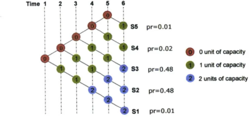
Time 1 2 3 4 5 6

S5 pr=0.01

S4 pr=0.02

*

S3 pr=O.48

~

S2 pr=0.48

Si pr=0.01

Figure 2-3: Scenario tree for comparison of the three existing GHP models

F251.

2.4.4

Example

Ramanujamn [251 describes the three models with the help of this example. Consider

the scenario tree given in Figure 2-3 and the flight schedule of two aircraft described

in Table 2.2.

If there was no ground holding policy, flight A would arrive at its destination at

t = 3. With a probability 0.51, the capacity will be 0. When this happens, the flight

will be put on an air hold until a landing slot is available. Suppose the ground holding

cost be 1/ aircraft /hour and air holding cost be 5

/aircraft/

problem is presented in Table 2.3. Both aircraft are given a deterministic ground

hold of 1 time period each. The aircraft arrive at t = 4 and t = 5 now. It is certain

that there will be a ground hold of 1 time period for both the flights. However,

there will be an air hold only in scenarios S4 and S5 (with probabilities 0.02 and 0.01

respectively).

The dynamic solution is presented in Table 2.4 and 2.5. Flight B gets different

26

Flight Original Arrival Time Ground Hold Revised Arrival Time

A 3 1 4

B 4 1 5

Table 2.3: Static slot reallocation.

S1 S2 S3 S4 S5 Original Departure 1 1 1 1 1 Original Arrival 3 3 3 3 3 Ground Hold 1 1 1 1 1 Revised Departure 2 2 2 2 2 Revised Arrival 4 4 4 4 4

Table 2.4: Dynamic slot reallocation for Flight A.

_________ _I

Table 2.5: Dynamic slot reallocation for Flight B.

amount of ground holds depending on the scenario. The scheduled takeoff time for

B is 3. At this time, S1 and S2 would have resolved themselves. If the scenario is

S1, then B takes off on time. Else, it is ground held. At t = 4, if the scenario is S2 or S3, the flight takes off or else it is ground held. Att = 5, if updated information

indicated the realization of S4, then B takes off, else it takes off at t = 6. Note that

we assume a very high capacity at t = 7, so that any remaining flights affected by

the GDP can land at that time.

Let us look at how an airline would swap slots under both the static and dynamic

allocation. Suppose that Flights A and B are operated by the same airline, and

that Flight B has a higher delay cost because it has a lot of connecting passengers.

Swapping is straightforward in the static assignment. Flight A and Flight B are

allotted a landing slot at t = 4 and t = 5 respectively. We will interchange these two

Table 2.6: Hypothetical case where Flight A dynamic model.

takes the slot assigned to B, through a

IS1 S2 I S3 S4 S5

Ground Hold

1

1

1

1

1

Revised Departure 2 2 2 2 2

Revised Arrival 4 4 4 4 4

Table 2.7: Hybrid slot reallocation for Flight A.

___________S1 S2I S3 IS4 S]

Ground Hold 0 1 1 1 1

Revised Departure 3 4 4 4 4

Revised Arrival 4 5 5 5 5

Table 2.8: Hybrid slot reallocation for Flight B.

B will land at t = 4, incurring a ground delay of 0. Thus, Flight B

and the airline can attain its objective.

takes off on time

On the other hand, we will not be able to perform this slot swap for the dynamic

allocation. This is because of the unequal flight durations associated with the two

slots. If Flight A was to take the slot assigned to B, the schedule would look as

shown in Table 2.6. This is an infeasible assignment since Flight A cannot distinguish

between Scenario S4 and S5 at departure time 4. The slot was meant to be for a flight

of duration 1, and not for a flight of duration 2. Thus swaps can only be made between

flights of same duration.

The hybrid formulation addresses this limitation of the dynamic model. The

resulting solution is presented in Table 2.7 and 2.8. If flight A were to take the slot

for B, there would be no ambiguity in resolving any scenario (as seen in Table 2.9).

The optimal pre-CDM costs in the static, hybrid, and dynamic allocations in this

28 IS1 S2 S3 S4 S5 Original Departure 1 1 1 1 1 Original Arrival 3 3 3 3 3 Ground Hold 1 2 3 4 5 Revised Departure 2 3 3 4 5 Revised Arrival 4 5 5 6 7

SI S2 S3 S4 5

Ground Hold 0 1 1 1 1

Revised Departure 2 3 3 3 3

Revised Arrival 4 5 5 5 5

Table 2.9: Hypothetical case where Flight A takes the slot assigned to B, through a hybrid model.

example are found to be 2.4, 2.39, and 2.23, respectively. The pre-CDM cost is lowest

for the dynamic model, followed by the hybrid and static model.

2.5

Collaborative Decision Making (CDM)

formula-tion

The response of the airlines to the initial slot allocation is discussed. This was first

presented by Ramanujam (2011) [251. We formulate the intra-airline slot

substitu-tion as an assignment problem. Then we discuss the incentives required for truthful

reporting of slot cancellations.

2.5.1

Intra-airline slot exchange

Once a GHP is solved by the FAA (using nominal values for C, and Cg,n), the following

information is sent to airlines for each of their flights

1. Minimum ground holding time: The minimum ground hold that will be assigned

to a slot s across all scenarios is grdmjn(s) .

2. Expected ground holding time: This is the average ground holding time that

will be assigned to the slot. For a slot s, the expected time is grd(s).

3. Expected air holding time: The airborne queue that a slot will experience is

dependent on the scenario. The scenario probability weighted mean wait time

The airlines have flight-specific delay costs. For each flight

f,

original schedule, every flight also has a departure time dep(f), along with a flight duration dur(f). The aim is to find a minimum cost matching of flights to slots.

Let Fa be the set of flights assigned to airline a. Denote the flight corresponding

to slot k as fk. The cost of assigning a flight

f

Cf,k = Cg grd(sk) + Cair(sk) f, fA G Fa (2.22) We define a 0-1 indicator variable to determine the feasibility of a slot swap.

feas(f, k) is 1 if the flight

f

feasibility is that the flight cannot take off before its original published time. This is

used as a surrogate for the earliest possible departure time of the flight. The necessary

condition for feasibility of swaps (feas(f, k) = 1), is dep(f) > dep(fk) + grdmin(sk). For the static and hybrid formulation, this is also a sufficient condition. For the

dynamic formulation, we have an additional restriction on the flight duration, i.e.,

dur(f) - dur(fk).

The optimization problem finds the minimum cost, scenario-independent

assign-ment of flights to slots.

min

E F

Xf,k < feas(f, k) Vf E -Fa, {k: fk E Fa} (2.26)

Xf,k C {0, 1} Vf E .Fa, {k: fk E Fa} (2.27)

Equations (2.24) and (2.25) are required so that a one-one mapping between flights

and slots is maintained. Equation (2.26) ensures only feasible swaps.

2.5.2

Slot Credit Substitution

Airlines might also respond to GDPs by canceling flights. Sometimes, it may be

cheaper to cancel a flight instead of delaying it by a lot. Since a flight has multiple

legs in its journey, it is also possible that an aircraft might not be able to use a slot

assigned to it. The Slot Credit Substitution (SCS) mechanism is triggered whenever

an airline decides to forfeit a slot. This is in contrast to the earlier compression

algorithms that were run in batches.

Ramanujam [25] describes three essential features of a SCS mechanism in the

stochastic context:

1. An airline which forfeits a slot c can request any later slot k.

2. All other flights see a decrease in air and ground delay (Pareto improvement for

all other flights).

3. The benefit of a cancellations must be distributed to all the flights in a equitable

manner.

The first two conditions ensure an incentive compatible mechanism for the airlines

to report slot cancellations, since they are going to be strictly better off if they report

a cancellation, or request a later slot. The last feature refers to the equitable manner

in which the benefits of a slot forfeiture are distributed among other airlines. Pareto

improvement requires that each flight has no increase in both the airborne queue

and the ground hold. This is a strong requirement. Although not addressed in this

thesis, it is possible to develop a broad definition of "improvement" in terms of airline

benefits. In the simulations described in Chapter 4, we will compute the system wide

benefits of implementing the SCS algorithm described in [25].

* The flight that is forfeiting its current slot assignment, c, and the later time slot that it requests, k

* Information regarding all the other flights

- _{ETA(slotf): The earliest arrival time of each aircraft assigned to slot f}

-W: The airborne queue length

- dur(slotf): Duration of the slot assigned to flight

f

- arrq(slotf): Arrival time of flight

f

The SCS optimization will try to allot a slot at time k or later to the airline that vacates c, and decrease the delay for all other feasible flights. The benefit (decrease in delay) for the canceled flight, the non-canceled flights, and the entire system, are computed in Chapter 4.

Chapter 3

Receding Horizon Static Ground

Holding Problem

In this chapter, we introduce the Receding Horizon Static (RHS) formulation for the

stochastic SAGHP. In the previous chapters, we studied the features of the static, dynamic and hybrid models. The static model was found to provide the least

pre-CDM benefits. However, it is the most flexible in terms of slot exchanges, and gives

the most benefit during the CDM step. By contrast, the dynamic model has the best

pre-CDM performance because it takes advantage of the latest capacity forecasts. But

the flight duration-specific slot assignment constrains slot swaps, resulting in the least

CDM benefits. This tradeoff motivated the development of the hybrid formulation

[27].

The hybrid formulation can make use of dynamic information available at every

time step and also ensure that slot substitutions are not restricted. Like the dynamic

model, there is a large communication overhead associated with it. At every time

step, the capacity estimates need to be shared among all the stakeholders. The

current branch of the scenario tree must also be common knowledge. Operationally, this can pose a challenge. Airlines cannot plan for future time steps because of the

uncertainties involved.

" Minimum cost: The primary aim of the optimization is to try and transfer all the delay to the ground instead of the air, and balance it against the risk

of starving the arrival runway. The Post-CDM cost is the primary metric for

evaluation (as opposed to the pre-CDM cost)

" Fair allocation of resources: This is an important feature for airlines. The ideal

allocation will not distinguish between flights of different duration, or airlines

with different market shares. Ration-By-Schedule (RBS) is accepted as a fair

allocation procedure by the airline industry.

" Robustness of algorithm: The length, severity (reduced capacity to nominal

capacity ratio), and scope of GDPs vary widely. The algorithm must therefore

show consistent performance in a wide range of scenarios

" Predictability: Airlines would like to know the departure time of their flights

well in advance. As per this consideration, static models are most preferable.

Also, once assigned, the schedule should preferably not change (which supports

the dynamic formulation of Richetta and Odoni [29] over that of Mukherjee and

Hansen [22]).

" Computational tractability of the formulation: The problem should not scale

exponentially with the number of flights involved.

3.1

RHS model

The RHS model is motivated by the following two favorable features of existing

mod-els:

o The static model gives a slot assignment well in advance of the GDP, and also

provides maximum flexibility to make intra-airline slot substitutions. Further, the static solution will also be a fair RBS allocation if the ground holding costs

are marginally non-decreasing [191.

* The strength of the dynamic formulation comes from its ability to use updated

capacity forecasts. We incorporate this feature into the RHS model by allowing

for multiple runs of the static model. Whenever a static solution is obtained, it

is implemented by airlines until the next run of the static optimization.

In this process, we hope to develop an alternative to the hybrid model which tries

to achieve the same purpose: a low post-CDM cost.

3.1.1

Terminology

Let the length of the GDP be T. The discrete time-steps are {1, 2, ... , T}. The static optimization is re-solved with updated information at specific times, denoted as the

"update times". Therefore, if we have k update times, ti, .., tk, with 1 < t1 < ... <

tk < T, then the static model will be run at times 1, t1, t2,..., tk. Whenever the static

model is run at time ti, a schedule is planned for times tj through T. The period

between two updates is denoted as a stage. The first stage is therefore from t = 1 to

t =t - 1, the second stage from t = ti to t = t2 - 1, and the (k + 1)th stage is from

t = tk to t = T.

Consider the scenario tree in Figure 3-1. Let the update times be t1 = 2 and t2 = 4. At t1 = 2, the occurrence or non-occurrence of S1 is known. Scenario S1 is

said to be resolved at time t=2. Scenarios S2 to S6 are still indistinguishable and are

said to be unresolved at that time. Now when the second update happens at t2 = 4,

S2 and S3 will get resolved (in addition to S1, which was already resolved). At t2,

scenarios S4 to S6 remain unresolved. In general, at any time t, scenarios S1,...,S(t-1)

would have been resolved.

We define a k-stage RHS formulation as one where the static model is run k times.

Since the model is always run at t = 1, there will be k - 1 update times. Specifically,

a 2-stage RHS model has one update time.

t, t2 t3 t4 t5 t6 S6 55 4C4 S4 S3 S2 OS1 Unresolved scenarios at t=4 Scenarios resolved at t=4 Scenario resolved at t=2

I

Figure 3-1: Example of resolved and unresolved scenarios.

3.1.2

Model

The RHS formulation is similar to the static model in many aspects. We however do

not use the decision variable Xij as shown in Section 2.4.1. In RHS implementation,

we need to keep track of flights across stages, and it is therefore important to know

the flight duration. We will instead use the variable X,,ij (defined below). It is to

be noted that this decision variable is not flight-specific. The formulation will not

distinguish between flights of different durations, unlike the dynamic model. This

variable is just needed for book-keeping purposes.

The RHS model is a generic framework based on rerunning the static model.

However, we will only present the details for a 2-stage version. The basic ideas

developed here can be generalized for any number of updates.

Step 1: Solve the static model at t=1

T T T+1 T

Minimize Cg,jiX9 Ii,j + E 7rq(Ca W' (3.1)

s=1 i=1 j=i qEQ t=1

T+1 subject to E X = Ns,, Vs E {1, ... , T},Vi E {1, ..,T} (3.2) j=i T t WI'>> X , + ' - M, Vt E {1,..,T},qEQ (3.3) s=1 i=1 W '4 = 0, Vq E Q (3.4)

Xf8,,

Q

X iij : Number of flights scheduled to take off at s and land at i, which are rescheduled to

land at

j.

W '4 : Airborne queue at time t for scenario q (decision variable for stage I of the GDP) t :Update time for the 2-stage RHS model

Ns,,i :Number of flights scheduled to takeoff at time s and land at time i (given from the original schedule)

Q

Equations (3.1)-(3.5) are similar to the static formulation in Section 2.4.1.

Step 2: Implement the solution until -I 1

X ij and W is the solution to the first optimization. All flights with a resched-uled take off time before i will follow the static solution. At t = t, the optimization

is going to be rerun.

Step 3: Run the second static optimization

The second run of the static model needs to consider the following issues at i:

1. Flights that have been ground held in stage I and have not yet departed: A

flight ground held through the first stage is reconsidered in the second stage

optimization problem. They are considered as new flights scheduled to take -1-1 - I 1 1, ,- -,

off at t. By revising their take off time to t, these flights will get preference over the other second stage flights and we retain the RBS property of the static formulation. It will get a revised takeoff time depending on capacity estimates. Define an auxiliary flight schedule matrix for stage II as NZ.

N8 {= N,i Vs i>t (3.6)

N!_, =Nil iX', Vs <t, (s + j-i) t (3.7)

Equation (3.6) considers the original schedule and (3.7) accounts for flights which are ground held.

2. Flights that have taken off at stage I but are currently airborne: Let the variable Rt E Z+, t > t denote the number of airborne flights from stage I which will be

landing in stage II. It is calculated according to (3.8)

Rt = Rt + Xs,i,t , t > i, { (s, i) : (s + t - 0) < i < t} (3.8)

3. The airborne queue from the first stage which gets handed over to the second

stage solver: We add the constraint that the initial queue for the second stage

is equal to that obtained form the first stage solution.

4. Scenario tree update: The second stage optimization ((3.11)-(3.15)) involves two

possibilities: a specific scenario is realized, or scenarios are unresolved. When a specific scenario, say q* gets resolved, then Q = {q*} and ireq = 1 (because it reduces to a deterministic problem). The probability of a scenario being unresolved at t = t is denoted by punres and in this case, we have Q = {t, ... , T}. The probabilities being used in the formulation are then conditionally updated as described in (3.9)-(3.10).

T

Punres = 7rq (3.9)

q=i 38

7rq

irq = Pr Vq c{t, ..., T}

Punres

(3.10)

5. Total cost of the two stage solution: This is evaluated after we have both the

stage solutions.

The second stage of the static optimization is solved considering the updated

inputs. The main difference in the second stage formulation are the use of the

up-dated flight schedule (Constraint (3.12)) and explicit accounting of airborne flights

(Constraint (3.13)).

T T T T

Minimize C ,_iX>, + 1 frq(Ca

>3

s=t i=t j=t qeQ t=t T subject to X " Nf, Vs, i > W

~

~

X E 2+, +/I,q E Z+,Vt,s,ij tVEQ,

(3.11) (3.12) (3.13) (3.14) (3.15) Notation:

XI,,: Flights scheduled to take off at s and land at i, which are rescheduled to land at j.

This solution is in stage II of the GDP (decision variable).

W I' : Airborne queue for stage II of the GDP planning at time t for scenario q (decision

variable).

N8'(: Number of flights scheduled to takeoff at time s and land at time i in the second

stage (from Equation (3.6) and (3.7)).

Q: Denotes the set of scenarios that are considered for the second stage.

irq: _{Probabilities associated with the resolved or unresolved scenarios in set}

Q.

W~*'Q: Optimal solution of the first stage airborne queue in scenario q.

The total delay cost for a 2-stage RHS is computed as the sum of the Stage I

stages are X*, 8,2,3 , 8,113 , W47*', and W'. ; I W The stage I cost is the ground holding

costs from t = 1 to t I

- 1 and the expected air delay for the same time period.

T-1

Cost=ZZZ Cmin(j-iS) _1X, + E 7Wq(Ca W (3.16)

S<i i>8 j':i qEQ t=1

The Stage II cost has two cases, one in which the scenario is resolved, and another

in which the scenarios are unresolved. When a particular scenario q is resolved in

Stage II, the cost is given by:

COSt Iq=

S S S

s>i i>s j i t>i

When the scenarios are not resolved, we update the expected cost as:

COStHI,unresolved =

5 5

s>t i>8 j>i qEQ t>i

The total cost of stage II is therefore a probability-weighted sum of the resolved

and unresolved scenarios:

Cost1 1 = Punres * COSt1I,unresolved +

5

q=1

The total cost of the solution is:

Total Cost = Cost1 + Cost11 (3.20)

3.1.3

Number and time of updates

An important question regarding the RHS model is the choice of the update time.

If the update time is t = 1, then we gain no additional information about scenario

occurrences. Further, if the update time is t = T, then all flights have already

followed the schedule decided by the first stage. Despite of the ability to identify the

scenario precisely, there are no flights that can benefit. There is a tradeoff between

early updates, with which we can potentially control a lot of flights in stage II, and

waiting for better capacity estimates. This optimal update time depends on the flight

schedules, reduced capacity estimates, probability distribution among the scenarios, and the length of the GDP. We do not study theoretical estimates, or formulate this

as an optimization problem in this thesis. Instead, we identify the optimal update

times through simulations. We illustrate this process with an example in the next

chapter.

The other important parameter is the number of updates. We described the

2-stage RHS model. If we increase the number of 2-stages, we obtain better capacity

forecasts, which will decrease the pre-CDM costs. Intuitively, if we have a static

update at every time step, we will have the lowest cost. However, this solution still

has a higher cost than the dynamic solution. When we have multiple updates to

make, we need to search from all possible permutations to find the optimal update

times. For example, if we decide to have k updates for a GDP of time horizon T, we

must find the update times from T! combinations. To summarize, the pre-CDM

costs have the following order

Cost [dynamic GHP] Cost [T-updates] <

... Cost[2-updates] Cost[static GHP]

3.2

Intra-airline substitution under the RHS

formu-lation

We will first summarize how the 2-stage RHS formulation is implemented. Suppose

a GDP of a certain duration and scope has been called due to a predicted

supply-demand imbalance. Since the system operator does not have airline-specific costs for

ground and air delays, for the sake of fairness, it assumes the same value for all flights.

It then solves a 2-stage RHS model, and determines the minimum delay cost solution

and the optimal update time. The system operator has the solution for the first stage, and a scenario-specific solution for the second stage. The following information is now