Application of an inverse model in the community modeling effort results

APPLICATION OF AN INVERSE MODEL IN THE

COMMUNITY MODELING EFFORT RESULTS

by

Huai-Min Zhang

M.S. in Physical Oceanography, MIT/WHOI Joint Program, 1991 Submitted in partial fulfillment of the

requirements for the degree of DOCTOR OF PHILOSOPHY

at the

MASSACHUSETTS INSTITUTE OF TECHNOLOGY and the

WOODS HOLE OCEANOGRAPHIC INSTITUTION February 1995

Q)Huai-Min Zhang 1994 The author hereby grants to MIT

and to distribute copies of this

Signature of Author ...

and to WHOI permission to reproduce thesis document in whole or in part.

Joint Program in Physical Oceanography Massachusetts Institute of Technology Woods Hole Oceanographic Institution December 14, 1994 Certified by... ... ... Nelson G. Hogg Senior Scientist Thesis Supervisor Accepted by... ... Carl Wunsch Chairman, Joint Committee for Physical Oceanography it; Massachusetts Institute of Technology

WVIT

APPLICATION OF AN INVERSE MODEL IN THE COMMUNITY MODELING EFFORT RESULTS

by

Huai-Min Zhang

Submitted in partial fulfillment of the requirements for the degree of Doctor of Philosophy at the Massachusetts Institute of Technology

and the Woods Hole Oceanographic Institution Dec. 12, 1994

Abstract

Inverse modeling activities in oceanography have recently been intensified, aided by the oncoming observational data stream of WOCE and the advance of com-puter power. However, interpretations of inverse model results from climatological hydrographic data are far from simple. This thesis examines the behavior of an inverse model in the WOCE CME (Community Modeling Effort) results where the physics and the parameter values are known. The ultimate hypotheses to be tested are whether the inferred circulations from a climatological hydrographic data set (where limited time means and spatial smoothing are usually used) represent the climatological ocean general circulations, and what the inferred "diffusion" coeffi-cients really are.

The inverse model is first tested in a non-eddy resolving numerical GCM ocean. Numerical/scale analyses are used to test whether the inverse model properly represents the GCM ocean. Experiments show how biased answers could result from an incorrect model, and how a correct model must produce the right answers.

When the inverse model is applied to the time-mean hydrographic data of an eddy-resolving GCM ocean in the fine grid resolution of the GCM, the estimated horizontal circulation is statistically consistent with the EGCM time means in both patterns and values. Although the flow patterns are similar, the uncertainties for the GCM time means and the inverse model estimates are different. The former are very large, such that the GCM time-mean circulation has no significance in the deep ocean. The latter are much smaller, and with them the estimated circula-tions are well defined. This is consistent with the concept that ocean mocircula-tions are very energetic, while variations of tracers (temperature, salinity) are low frequency. The inverse model succeeded in extracting the ocean general circulation from the

"climatological" hydrographic data.

The estimated vertical velocities are also statistically indistinguishable from the GCM time means. However, significant differences between the estimated

"dif-fusion" coefficients and the EGCM eddy diffusion coefficients are found at certain locations. These discrepancies are attributed to the differences in physics of the inverse model and the EGCM ocean. The "diffusion" coefficients from the inversion parameterize not only the eddy fluxes, but also (part of) the temporal variation and biharmonic terms which are not explicitly included in the inverse model.

Given the essentially red spectrum of the ocean, it makes sense to look for smooth solutions. Aliasing due to subsampling on a coarse grid and the effects of spatial smoothing are addressed in the last part of this thesis. It is shown that this aliasing could be greatly reduced by spatial smoothing. The estimated horizontal circulation from the spatially smoothed time-mean EGCM hydrographic data with a coarse grid resolution (2.40 longitude by 2.0* latitude) is generally consistent with the spatially smoothed EGCM time means. Significant differences only occur at some grid points at great depths, where the GCM circulations are very weak.

The conclusions of this study are different from some previous studies. These discrepancies are explained in the concluding chapter.

Finally, it should be pointed out that the issue of properly representing a GCM ocean by an inverse model is not identical to the issue of representing the real ocean by the same inverse model, since the GCM ocean is not identical to the real ocean. Numerical calculations show that both the non-eddy resolving and the eddy-resolving GCM oceans used in this work are evolving towards a statistical equilibrium. In the real ocean, the importance of temporal variation terms in the property conservation equations should also be analyzed when a steady inverse model is applied to a limited time-mean (the climatological) data set.

Thesis Supervisor: Dr. Nelson G. Hogg Senior Scientist

Table of Contents

Abstract

1. INTRODUCTION

1.1 INVERSE MODELING IN PHYSICAL OCEANOGRAPHY .... 1.2 EXAMINATION OF INVERSE MODELS...

1.3 THE APPROACH OF THIS WORK ... 2. THE MODELS

2.1 INTRODUCTION ...

2.2 THE NUMERICAL OCEAN GENERAL CIRCULATION MODEL 2.3 THE INVERSE MODEL ...

2.3.1 Introduction ...

2.3.2 Formulation of the Equations ... 2.3.3 Surface Layer Model ... 2.3.4 Finite Difference Formulation ... 2.4 SUM M ARY ...

3. APPLICATION OF THE INVERSE MODEL RESOLVING NUMERICAL GCM OCEAN 3.1 INTRODUCTION ...

IN A NON-EDDY 44

44 3.2 ACCURACY OF THE INVERSE MODEL ASSUMPTIONS IN THE

NON-EDDY RESOLVING GCM OCEAN ... 46

3.2.1 Dynamic Equation ... 46

3.2.2 Conservation Equation for Water Properties ... 50

3.3.1 Introduction . . . . 3.3.2 Upper-Layer Model Results Without Surface Frictional Layer

(U L M ) . . . . 3.3.3 _{Experiments on the Ekman Pumping Velocity Constraint . .} 3.3.4 Model with Frictional Surface Layer-Determine the Air-Sea

F luxes . . . .. . . . . 3.3.5 Deep-Layer Model (DLM) . . . . 3.3.6 A Full-Layer Model-Can We Make Consistent Estimates? 3.4 EXPERIMENTS ON THE PARAMETERIZATION . . . .

3.4.1 Introduction . . . . 3.4.2 A, K, w and Air-Sea Fluxes as 3rd Order Polynomials-PAR I 3.4.3 A, K and Air-Sea Fluxes as 3rd Order Polynomials while w is

a Point-wise Unknown-PAR II . . . . 3.4.4 D iscussion . . . . 3.5 SUMMARY AND CONCLUDING REMARKS . . . .

56 62 69 83 91 93 110 110 112 120 125 126

4. APPLICATION OF THE INVERSE MODEL IN AN EDDY-RESOLVING

NUMERICAL GCM OCEAN 132

4.1 INTRODUCTION ... ₁₃₂

4.2 THE NUMERICAL GCM OCEAN ... 135

4.3 _{INVERSION OF THE TIME-MEAN FIELDS ... 145}

4.3.1 Introduction ... . 145

4.3.2 _{Accuracy of the Inverse Model in the Time Mean Fields of} the EGCM Ocean ... ... 147

4.3.3 _{Inverse Model Results of the Time-Mean Fields ... 153} 4.3.4 Summary and Discussion ... 1777

4.4 APPLICATION OF THE INVERSE MODEL IN THE SPATIALLY SMOOTHED TIME-MEAN FIELDS OF THE EDDY-RESOLVING GCM OCEAN ... ... 180 4.4.1 Introduction ... . 180 4.4.2 Subsampling Aliasing-the Accuracy of the Inverse Model in

a Coarse-grid Resolution ... 182 4.4.3 Inverse Model Results in the Spatially Smoothed Time-Mean

O cean . . . 196 4.4.4 _{Sensitivity of the Inverse Model Results on the Vertical Level}

(Layer) Number ... ... 218 4.4.5 Summary and Discussion ... ... 221

5. CONCLUSION AND DISCUSSION 225

APPENDIX A: SPATIAL SMOOTHING AND FINITE-DIFFERENCE

GRADIENT ₂₄₆

Acknowledgments ₂₅₃

Chapter 1. INTRODUCTION

This thesis extensively examines one of the many inverse models used in the field of physical oceanography in the context of the WOCE CME results (Community Modeling Effort of the World Ocean Circulation Experiment). This chapter describes the motivations, background, and methodology as well as the organization of this thesis.

1.1

INVERSE MODELING IN PHYSICAL

OCEANOG-RAPHY

Inverse methods have been widely used in many fields of science and en-gineering. As one example, the use of inverse methods in medical imaging has recently been reviewed by Louis (1992). Their use in geophysics was described by, for example, Backus and Gilbert (1967), and was summarized in a textbook by Menke (1984). The introduction and systematic study of inverse methods in physi-cal oceanography has been carried out by Wunsch (e.g., Wunsch, 1977, 1978, 1984, 1988a, 1994) and other physical oceanographers (e.g., Bennett, 1992).

Inverse models in physical oceanography address of the inadequacies of tradi-tional methods (the descriptive method and the dynamic method) for determining the ocean circulations. One of the major goals of physical oceanography is to de-scribe the large-scale time-mean circulation in the world oceans. Determining the general ocean circulation is an important step toward understanding the global climate system (e.g., the global budget of heat, fresh water, C02, etc.), the

distri-bution of water properties (temperature, salinity, etc.) and chemical tracers as well as biological nutrients and sediment movement in the oceans.

Unfortunately, compared to atmospheric observations, direct measurements of the circulation in the world oceans are much more difficult and costly. Typically available are the in situ measurements of hydrographic data and chemical tracers from individual cruises. The two traditional means to deduce the oceanic circulation from these available information are the so called descriptive method and dynamic method. The descriptive method uses the spatial distribution of water proper-ties to "draw" the directions of the water movement qualitatively (e.g., Wfist's, 1935, core-layer analysis; Montgomery's, 1938, isentropic analysis). No quantita-tive computations can be made from these methods. In addition, as the water property distributions involve both advective and diffusive processes, the "arrows" drawn along a water "tongue" can be incorrectly interpreted. Examples of similar property fields resulting from different physical processes were found in Zhang and Hogg's (1992) inversion in the Brazil Basin. Although coincidence of flows along temperature (and salinity) tongues on the isopycnals was found in one region, cases of flows along isotherms were also found in other regions.

The dynamic method utilizes the density field of observations to calculate the vertical shear of the horizontal velocities through the geostrophic and hydro-static balances (the thermal wind relation). Both theory (e.g., Pedlosky, 1987) and observations (e.g., Bryden, 1977) show that the large scale oceanic circulations are mainly in geostrophic balance, although there are violations of this assump-tion in some regions of the ocean (e.g., in the boundary layers). But there is a difficult issue to deal with in this method. Intrinsically the dynamic method can only give us the vertical shears or differences of the lateral velocities between two

surfaces. To determine the absolute velocities in the water column (assuming the geostrophic assumption is valid), the absolute velocity at a certain depth must also be prescribed. This traditionally involves the so-called "level-of-no-motion" or the velocity at the "reference level". Although various ways to determine the "level of no motion" have been proposed (e.g., the ocean bottom or at certain deep depth, or an interface of two different water masses which appear to be flowing in opposite directions), there are neither theoretical, nor observational justification for the ex-istence of a level of no motion. Small errors in the reference velocities can produce large errors in calculating the heat and other water property transports across a basin scale hydrographic section.

The determination of the "reference level" velocity stimulated the growth of inverse models in physical oceanography (Wunsch, 1977, 1978; Stommel and Schott, 1977; Schott and Stommel, 1978). The velocities calculated from the dy-namic method alone (from the thermal wind relation) do not ensure flows consistent with the distribution of tracer fields. Inverse models sought to remove these inconsis-tencies by requiring the circulation to simultaneously satisfy a variety of constraints deduced from the observed property distributions. Multiple conservation equations to determine water transports were also used in earlier work by Hidaka (1940), Riley (1951) and Wright (1969).

Since the pioneering work of Wunsch (1978) and Schott and Stommel (1978), a variety of inverse models have been developed with differing degrees of complexity applied mainly in the North Atlantic (due to the relatively dense coverage of hy-drographic sections in this ocean basin), and a few of other basins. Wunsch (1980) described the problem of combining hydrography with marine geodesy and satellite altimetry for the purpose of determining the general circulation of the oceans,

defin-ing the eddy field, and improvdefin-ing the marine geoid. In early box inverse models, it appears that the problem is underdetermined, leading to a range of circulation patterns compatible with geostrophic balance and the conservation of mass (e.g., Wunsch and Grant, 1982). In this case one usually gets an infinite set of solutions instead of getting the solution. Wunsch (1984) argued that the range of possible oceanic solutions could be narrowed by adding to the inversion information derived from other data sets (direct velocity or tracer measurements). Using an eclectic model, Wunsch (1984) succeed in putting useful bounds on the meridional flux of heat in the North Atlantic ocean. Olbers et al. (1985) applied the beta-spiral method to the North Atlantic data and, in addition to the determination of the absolute flow field, showed that the method could be used to infer diffusion rates. The method appeared to work well in areas where diffusion was a dominant process in the tracer balance, but the results were less compelling where this was not the case. In Joyce et al.'s (1986) work, data from a shipborne acoustic profiling device have been combined with hydrographic sections across the Gulf Stream and are used to estimate the absolute flow fields. The inverse results for the Gulf Stream transports are plausibly close to previous calculations. Inversions were also done individually on the Doppler data and the hydrographic data. They concluded that the inversion of the combined data sets produces results much improved over those using either acoustic or hydrographic constraints in isolation.

The more complicated inverse models are designed to infer not only the ab-solute velocities, but also the mixing rates in the ocean. Mixing has been proven to be an important process in water property balances, especially in the deep ocean where advection is weak. Using simple models, Tziperman (1987) also showed the importance of mixing processes in driving the deep thermohaline circulation and for

determining the basic vertical density stratification of the wind driven circulation. Knowledge of mixing rates are also important for (forward) numerical ocean mod-eling, such as the CME, as experiments have shown that GCM results are sensitive to the specific parameterization of the eddy diffusivity (Bryan, 1987). However, in practice the eddy diffusion coefficients from the inversions are very sensitive to data noise (e.g., Olbers, 1989). Oxygen, nutrients, tritium, radiocarbon and other tracers have all been used to constrain the inverse model solutions for these pa-rameters (Wunsch, 1984; Olbers et al, 1985; Hogg, 1987; Jenkins, 1987; Schlitzer, 1987; Spitzer et al, 1989). Their usefulness is usually determined by adequacy of knowledge of the measurement errors (e.g., instrumental and sampling problems) and of the sources and sinks for the tracers. The use of transient tracers for de-termining ocean transport is a more difficult problem. A first step towards making inference from sparse transient tracer information was taken by Wunsch (Wunsch, 1988a). Later he treated this problem using control theory (Wunsch, 1988b). These approaches are reviewed, together with other inverse problems and techniques, in a lecture in the NATO-Advanced Study Institute (Wunsch, 1989). A later application in the North Atlantic ocean was carried out by Memery and Wunsch (1990).

Development of inverse models in oceanography has taken more complicated forms. An example of the use of linear programming methods in the context of oceanographic tracer models in studying nutrient and carbon cycles in the North Atlantic is shown in Schlitzer (1989). Linear programming appears to be a pow-erful tool to examine the whole range of possible solutions. The method provides diagnostics to identify how well the model parameters are determined and which parts of the data provide important/redundant information. It is often possible to determine what additional information is needed to improve the solutions for

cer-tain parameters. Taking account the errors associated with each data set explicitly (by allowing the density field to be adjusted by the inverse model), Mercier (1986, 1989, 1993) formulated nonlinear inverse problems. Nonlinear optimization was also used by Wunsch more recently in the North Atlantic (Wunsch, 1994). Methods based on adjoint equations are not new but have recently attracted much interest as they become feasible to large systems. They are particularly appropriate for time-dependent systems with a large numbers of variables (e.g., initial or bound-ary conditions) for which optimum values are sought, and are widely used in data assimilation. Examples are Tziperman et al (1989), Marotzke (1992), Marotzke and Wunsch (1993), Schlitzer (1993), Schiller and Willebrand (1994), and Schiller (1994).

The recent increase of inverse model applications in oceanography is linked to the availability of more accurate data to constrain the parameter solutions. In the early stages of inverse modeling in physical oceanography, extensively used were the "box" inverse models due to the fact that the observations in the ocean were rarely adequate to compute the gradients needed in the "finite difference" mod-els. WOCE provides the opportunity to utilize the finite difference inverse models more efficiently in the ocean (one of the recent examples was Martel and Wunsch, 1993a,b). In fact, in addition to the observations, ocean modeling is another goal of WOCE. The two key modeling objectives of WOCE are to develop ocean models for predicting climate change and to develop methods for analyzing the WOCE field data. The analyzed WOCE data sets will be used to initialize and test models and to study long term changes in the ocean circulation. (WCRP, WOCE Report No.

In WOCE, temperature and salinity fields are measured to give information on the large scale baroclinic (vertically varying) velocity field. Surface drifters and other floats are being released to obtain direct information about the absolute velocity field. Satellites are being used to measure the wind stress on the ocean and also the ocean surface topography (giving the surface geostrophic velocity field). The data sets anticipated from WOCE will come close to defining the physical and chemical state of the ocean. A combination of in situ observations of hydrography and chemistry with altimetry, windfields (from both scatterometry and conventional analyses), float trajectories (e.g., Owens, 1991), current meter measurements, and direct estimates of water mass fluxes across various straits and sills (e.g., Bryden et al, 1994) ought to vastly reduce the existing uncertainty over the state of the ocean circulation. This will result in a global dataset of unprecedented scope. Given the oncoming data stream, an important issue is how to use these data to understand the climate state of the ocean and its physics (e.g., the general circulations, mixing rates, etc.).

1.2

EXAMINATION OF INVERSE MODELS

Although inverse models are widely used in physical oceanography, the in-terpretation of the inverse model results is far from simple, and the issue of the "validation" of the inverse models, i.e. whether the inverse model results represent the real ocean, is still not resolved. There are two aspects in this issue: first, the physics of the inverse model are not the same as those of the ocean; and secondly, inverse model solutions are not unique. The inverse model physics are usually much simpler than the ocean physics. Also, instead of getting the solution from an

in-verse model, one usually get a solution based on one's own criteria. For example, a box inverse model usually results in an underdetermined system, and the pa-rameter norm, or the kinetic energy at the reference level, is minimized in solving the equations (e.g., Wunsch, 1978). Some finite difference inverse models result in overdetermined systems (e.g., Hogg, 1987), and the residual norm of the equations is minimized to obtain the parameter solutions. In forward modeling, there are also subjective factors. First, different numerical models have different physics, and they are simplified versions of the physics in the real ocean. Secondly, there are various parameters which must be subjectively chosen. For instance, atmosphere forcing (wind stress, heat flux, etc) has large statistical uncertainties. Any values within the statistical errors are valid and there is no significant difference among them. In this sense, the forward modeling results are also not unique.

The essential question here is to what extent the inverse model results resem-ble reality. For the same reason that inverse models in physical oceanography were developed, the lack of direct observations of the circulations in the oceans makes it difficult to test the inverse models in the real ocean. Direct measurements of velocity in the ocean are rare, and one may doubt the representativeness of the comparisons of the measurements with inverse model results. One can argue that even if the comparisons show consistency at the very few measurement "spots", in terms of large scale ocean circulation, it still may not be consistent in the vast unmeasured area; and vice versa. Also, current meter measurements are usually taken over a very limited time period, while the estimated circulations by inverse models from hydrographic data are intended to be climatological. Reid et al (1977) reported deep/abyssal current meter measurements whose daily means have large variations within two months in the vicinity of the Vema Channel, although the measurements

are quite steady within the channel. More recent example are Schmitz and Hogg (1983), Tarbell et al. (1994). The strong eddy fields make the extraction of the weak ocean general circulation difficult.

A natural choice for testing the inverse models is to apply them in (forward) numerical model results. Fiadeiro and Veronis (1984) tested two inverse models in a highly idealized channel model. With the advance in computer power, more and more sophisticated (forward) numerical models have been/are being developed, with the aim to simulate the physical processes in the real ocean. Testing the inverse models in these numerical oceans is an important step toward understanding the functioning of the inverse models and the interpretation of the inverse model results. Historically the numerical general circulation models (GCMs) for the ocean come in two varieties. On one hand are models with active thermodynamics and moderate to high vertical resolution, but low horizontal resolution (the Non-eddy Resolving Models or the so-called OGCMs-the Ocean General Circulation Models). These have been developed in an attempt to represent the large-scale hydrographic structure and climatic properties (water mass formation rates, heat and fresh water transports, sea surface temperature anomalies, etc.) of individual basins or the world ocean. The strong dissipation required to maintain numerical stability in these low resolution models inhibits realistic hydrodynamic instabilities as well. This class of models has been moderately successful in simulating the mean ocean circulation and hydrographic structure of the world ocean (e.g., Bryan, 1979), and the variability of the upper ocean circulation where the variability is primarily wind forced (e.g., Sarmiento, 1986; Philander et al., 1987). The inverse model studied in this thesis will be first examined in one of these numerical OGCM oceans.

On the other hand, there are models with high horizontal resolution, but low vertical resolution, and generally incomplete treatment of thermodynamic processes (the Eddy-resolving General Circulation Models-EGCMs). These have been de-veloped in order to investigate the dynamics of time-dependent circulation systems including mesoscale eddies and their interactions with the mean flow (e.g., Holland, 1986). Thermohaline processes are difficult to incorporate into these models and they are limited to non-global domains in the early stage.

Advances in computer power are leading to a blurring of the distinction be-tween the OCGMs and the EGCMs, and have facilitated the convergence of these two modeling approaches. Basin- to global-scale simulations which include both representation of thermodynamic processes responsible for water mass formation and sufficient horizontal resolution to allow the hydrodynamic instabilities respon-sible for eddy formation have become fearespon-sible (e.g., Semtner and Chervin, 1988; F. Bryan and Holland, 1989). The inverse model studied in this work will also be tested in one of these GCM oceans (we will label it with EGCM).

Schott and Stommel's original

#-spiral

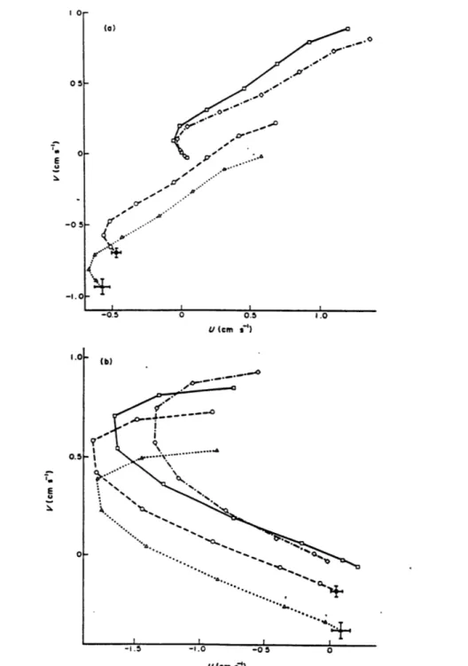
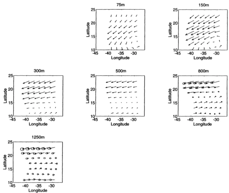
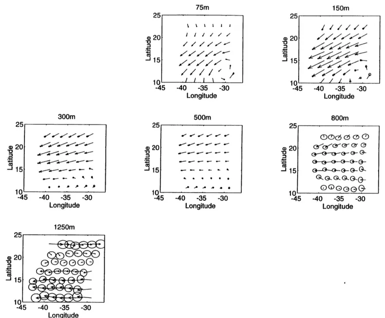
An intercomparison of three inverse models (the box model of Wunsch, 1978; the beta-spiral model of Schott and Stommel, 1978; and the Bernoulli model of Killworth, 1986) was made by Killworth and Bigg (1988) in the domain of a tradi-tional (with highly simplified topography) eddy-resolving general circulation model (EGCM) ocean (Cox, 1985). Two "scores" were defined for the inverse models: one tests point-wise accuracy (the "global" score), and the other tests flux of mass through a section (the "flux" score). They concluded that the Bernoulli method yields accurate global scores except in the homogenized region; the box inversion yields fairly accurate global scores everywhere, and the beta-spiral only gives accu-rate global scores near the equator. No method gives reliable flux scores, although the box inverse was the least inaccurate. The estimated velocities by the beta-spiral method are different from the GCM data (Fig. 1.2). In this figure, the arrows are the f-spiral method estimated velocity vectors, whereas the ellipses are the 5% er-rors of the corresponding time-mean GCM velocity vectors (from the tails of the shown vectors to the centers of the ellipses). More profoundly, they showed that a hypothesis of no flow at the ocean bottom gives predicted velocity fields (by thermal wind relation) which are closer to the "data" than any of the inversions in most cases.

Although the GCM statistical errors were shown, no estimated error infor-mation from the inversions was available, and as a result, we cannot judge the significance of the above velocity differences. Possible reasons for the "failure" of the inverse models in their GCM oceans will be analyzed in Chapter 5, in compar-ison with our conclusions.

S0- 05- 0-

-05-4

Fig. 1.1. Absolute velocity profiles at two points of a GCM ocean and various #-spiral inversions. ...A...: no diffusion terms; -o-: horizontal diffusion-only; -0--: both diffusion terms; ---GCM profile. (Bigg, 1985)

VeLoc-sty at depth = 174.0 m 42- 0 0 0 0 p. -W -lob 410 _{0 0 0 0} 400. 0p.O, 39 8 48 49 50 51 52 VeLoci.ty at depth = 223.5 m O C 0 C-48 49 50 51 52 VeLacLtyg at depth = 351.8 m 48 49 50 51 52 48 49 50 51 52

Fig. 1.2. Velocity vectors from a mass-conserving #-spiral inversion. The scale of 1 cm/s is shown. The tail of the vector is at the point concerned; the ellipse shows the 5% error (95% score) boundary. (Killworth and Bigg, 1988)

1.3

THE APPROACH OF THIS WORK

The conclusions of the above two papers raises doubts about the reliability of the inverse models, especially those derived from the beta-spiral method. A complete analysis of inverse model results should include all the error information. Oceanography has reached a stage of maturity such that estimates of parameter values without corresponding estimates of error no longer seem very useful. It should also be pointed out that, first of all, inverse model results to some extent depend on specific inverse techniques (e.g., scalings of the equations-row scaling, and scalings of the unknowns-column scaling). Secondly, the original beta-spiral method does not include the conservation equations of heat and salt as well as other tracers. Adding these conservation constraints will provide more information and the parameter solutions should be improved in terms of statistical closeness (with estimated uncertainties) to their "true" values, and/or in terms of the so-called solution resolution, which indicates how well the parameters are resolved (for detailed discussions, see Wunsch, 1989, or Zhang and Hogg, 1992). The reliability of this kind of inverse model has not been examined, and this is the objective of this work. Also, with all the information available from the numerical GCM results, detailed study of the terms controlling the inverse solutions (the effects of the data "noise") and appropriate interpretation of the estimations will be examined. Experiments on the parameterization of some variables will also be carried out in the hope of getting some guidance in applying the inverse model to the real ocean. The term "validation" of a model by a dataset must be used with caution. If the data physics is different from that of the model, we can not say that the model is "validated" by the data. Comparing the physics of the data and the model physics

is the first step toward examining a model. In this study, the analysis involves three "oceans": the real ocean (I), the forward GCM ocean (II) aiming at predicting the evolution of the real ocean, and the inverse model ocean (III) which was originally introduced to reveal the major features of the real ocean from hydrographic data and other observations. The three "oceans" usually do not have exactly the same physics and statistics, and they should be distinguished among each other. The question of whether (II) properly (within the statistics) represents (I) should be separated from whether (III) properly represents (I) or (II).

In testing an inverse model in the domain of the GCM oceans, we should first examine how accurately the inverse model reproduces the GCM oceans, or whether (III) sufficiently represents (II) within the statistical confidence limits. If the answer is yes, we would expect that the statistical inference by (III) from the hydrographic data of (II) should produce/recover the correct answers of (II). Otherwise we must conclude that the inverse model "failed", which is unlikely. On the other hand, if there are some discrepancies between the physics of (III) and (II), not all the parameters could be produced "correctly". The most interesting part in this case is how "well" each parameter is reproduced. In other words, we should ask which parameters are "correctly" produced (i.e. statistically consistent with their "true" values), and which are not. Note that in this case even though the inverse model "failed" to produce the "correct" answers for the GCM ocean, one cannot conclude that the inverse model would also fail to produce the correct answers for the real ocean. As pointed out before, GCM oceans differ from the real ocean. Failure of properly representing (II) by (III) does not necessarily imply failure of properly representing (I) by (III). Consistent statistical inferences can still be achieved for the real ocean if it can be properly represented by the inverse model.

The inverse model being tested in this work was originally developed by Hogg (1987) in isopycnal (potential density) coordinates. The major assumptions in this model are that the large scale oceanic circulations are in approximate geostrophic and hydrostatic balance, and mass, heat, potential density, and other tracers are approximately conserved in steady state. This model is of finite difference type.

In most traditional inverse models, velocities at the reference level are the unknowns, and the velocities at other depths are computed from the reference-level velocities after the inversion through the exact satisfaction of thermal wind relation. Hogg's model solves for the absolute velocities on all the depths (levels) simultaneously. Like the conservation equation (of heat, potential density, oxygen) constraints, the dynamic equation (thermal wind relation) is just another constraint (on the absolute lateral circulations), and the equations are solved simultaneously. Residuals are allowed in the dynamic equation as well as in the conservation equa-tions, and exact satisfaction of geostrophy/thermal wind relation is relaxed.

In Zhang and Hogg's (1992) (hereafter as ZH) application of this inverse model in the Brazil Basin, several modifications of the inverse model have been made. In Hogg's (1987) formulation and application in the central North Atlantic ocean, the Montgomery streamfunction, which was formulated for the specific vol-ume or specific volvol-ume anomaly surfaces (Montgomery, 1938), was used on isopycnal surfaces in its original form. What is implied in this application is the neglect of the variation of specific volume (anomaly) along isopycnal (potential density) sur-faces. In ZH it was shown that this variation may have dynamic importance in some regions of the ocean. By including the major part of this variation, new streamfunctions for the isopycnal surfaces were proposed. The second modifica-tion of the inverse model is in the ways of using the conservamodifica-tion equamodifica-tions. Hogg

(1987) used a simplified conservation equation for potential density together with the use of conservation equation for heat. The implicit assumptions used were that the thermal/saline expansion/contraction coefficients are constant (independent of temperature and salinity and thus of space), and that both the horizontal and ver-tical diffusion coefficients for heat and salt (and other tracers like oxygen) are the same. These might not be true in some regions of the ocean, especially where dou-ble diffusion occurs (e.g., McDougall, 1987; Schmitt, 1994). In addition, potential density is a derived quantity from potential temperature and salinity through the equation of state. Therefore, to avoid possible errors from the above approxima-tions, ZH used conservation equations for both heat and salt instead of for heat and the simplified density (among the three only two are independent). In the multi-layer model (total of eight vertical multi-layers extending from 250 m depth to 3500 m depth) in the Brazil Basin, ZH found that the inverse model estimated circulations in the upper ocean are consistent with previous studies (e.g., Reid, 1989; Defant, 1941). In the deep ocean, solutions are consistent with some previous work (e.g., Defant, 1941; Fu, 1981), but differ from others in small scale structure (e.g., Reid, 1989).

Experience in using this inverse model in the real oceans (and also in the numerical GCM oceans in the later chapters of this work) shows that this model normally results in an overdetermined system (in the traditional sense) and of full rank. Thus the solutions are obtained by minimizing the equation residual norm (in the least square sense), and no constraints on the parameter (solution) norm are used. In an underdetermined system, or an apparently overdetermined system with deficient rank, the solution (parameter) norm, or a combination of solution norm and equation residual norm is minimized in obtaining the solutions. For the

problems formulated for reference velocity what is usually minimized is the kinetic energy at the reference level and thus the choice of the depth of the reference level is important in these cases. In this sense Hogg's formulation is more objective but there are still subjective factors as well in this model (like the row scaling).

The thesis is organized in the following way. First, the physics and assump-tions used in both the numerical ocean general circulation model and the inverse model are briefly described and compared in Chapter 2. Then the inverse model is applied to a simple, non-eddy resolving GCM ocean (Chapter 3), to see how well it functions there. Several issues, such as the Ekman pumping velocity constraint, determining the air-sea heat and fresh water fluxes, effects of data "noise" on the solutions, the effects of temporal variation terms, as well as parameterization of diffusive variables, are pursued in this chapter. In Chapter 4, the results of the ap-plication of the inverse model in a more recent CME (EGCM) ocean are discussed. The model is first applied to the time-mean fields of the numerical GCM ocean, with the fine grid resolution of the GCM. The inverse model estimated circulations are compared with the time-mean GCM circulations, to see the ability of the inverse model to recover the time-mean circulations from time-mean hydrographic data. Also compared are the "eddy" diffusion coefficients from the inverse and those from direct computations of the eddy fluxes. The next part of this chapter examines ef-fects of spatial smoothing and larger grid spacing, which are usually used in the real ocean, on inverse model solutions. Finally, discussions and conclusions are given in

Chapter 2. THE MODELS

2.1

INTRODUCTION

As described in the previous chapter, the main purpose of this work is to examine whether useful inferences of the ocean state can be made by an inverse model from hydrographic data. Because of the lack of the needed information in the real ocean with which to compare the inverse model results, the examination is based on the numerical ocean general circulation model modeling results. In this study, the fields of water properties (potential temperature, salinity etc.) of simplified oceans generated by numerical ocean general circulation models (GCMs) are used as data for the inverse model, and the parameters for horizontal and vertical velocities and horizontal and vertical diffusion coefficients are estimated by solving the inverse model equations. Although these parameters are also known in the idealized numerical oceans, they are not used to constrain the inverse model solutions. Instead, they are used to compare with the inverse model results. This procedure is based on the notion that if the inverse model were applied to the real ocean, such information is generally not available.

As mentioned in Chapter 1, in order to fulfill the above objectives and to make meaningful analyses of the inverse model results, a complete understanding of the physics and assumptions of both the numerical GCM and the inverse model is essential. If the inverse model has the same physics and assumptions as the numerical GCM, or the differences are numerically negligible, we would expect the inverse model estimations to be completely consistent with those of the numerical

those producing the input data is difficult to achieve. For one reason, the GCM oceans are not completely in steady state, while the inverse model is a steady one. For another, the momentum equations in the GCM are unsteady and nonlinear, while the inverse model assumes geostrophic and thermal wind balances. With these subtle differences of the physics and assumptions, the question of whether we have the ability to utilize inverse techniques to make useful parameter estimations for horizontal and vertical velocities, diffusion coefficients, as well as air-sea heat and fresh water fluxes when the surface layer is included, is the main theme of this study.

First the numerical ocean general circulation model will be briefly described. Then the assumptions and formulations of the inverse model will be introduced. Finally, comparison of the two models will be made.

2.2

THE NUMERICAL OCEAN GENERAL

CIRCULA-TION MODEL

The numerical ocean general circulation model used to simulate the ocean cir-culations and water property distributions is the three-dimensional primitive equa-tion model of the ocean developed by the Geophysical Fluid Dynamics Laboratory (GFDL) of NOAA at Princeton University (Bryan, 1969; Cox, 1984). The model momentum equations are the simplified non-steady, non-linear, Navier-Stokes equa-tion with three basic assumpequa-tions: the Boussinesq approximaequa-tion, in which density differences are neglected except in the buoyancy term; the hydrostatic assumption, in which the equation of vertical motion is simplified by neglecting local acceleration and other terms of equal or smaller order; and the turbulent viscosity hypothesis

which is used to parameterize the stresses exerted by sub-grid scale motions. Water property changes (potential temperature, salinity, etc.) are obtained by integrating the non-steady conservation equations forward in time, again utilizing a turbulent mixing hypothesis to represent the sub-grid cell processes. The equations are linked by a simplified, but nonlinear equation of state.

In spherical coordinates, the continuous form of the equations are as follows:

au m

a(uu)

1(wu)

Re

aA

[am

(uv)

+

+

+

+fu

'au

a(v/m)]

aw

at

a

9

a$

+

oz

at+

[e

+

a

]+

az

M

(p/po)

where

#

#,

#,

f

FU = AMH

$R

AMV0

+

+

+

and Aab is the mixing coefficient for momentum and tracers (denoted by the first subscript M and T) and in the horizontal and vertical directions (denoted by the second subscript H and V). Note that vertical mixing is specified to be uniform under statically stable conditions

(?

un-stable conditions

(2

will be used in Chapter 4, the second order Laplacian dissipation described above is replaced by a fourth order biharmonic horizontal dissipation. The equation of state, eq.(2.6), is approximated as a nine-term, third-order polynomial in temperature and salinity (Bryan and Cox, 1972).

The "rigid-lid" assumption of zero vertical velocity at the surface of the ocean and the assumptions of no normal flow and no normal tracer fluxes at solid boundaries are adopted. Specifications of the values of turbulent viscosities AMH and AMy, and diffusivities ATH and ATV, as well as the surface boundary conditions (wind stress, air-sea heat and fresh water fluxes) will be discussed later together with the analyses of the corresponding numerical GCM results.

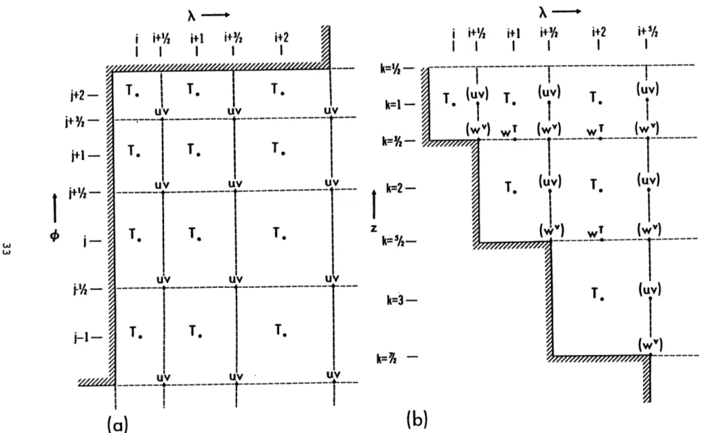
The finite difference formulation and the arrangement of variables within the cells correspond to the "B-grid" configuration of Arakawa and Lamb (1977). Horizontally, the grids for T and the grids for u, v are staggered, with T grids situated in the centers of the cells, and u, v grids placed at the corners of the cells (Fig. 2.1a). Vertically, the grids for T, u, v are located halfway through the vertical dimension of the cells, while the grids for w are located at the horizontal interfaces of the cells (Fig. 2.1b). Two sets of vertical velocities, wT and w", are calculated through the diagnostic continuity equation, at the interfaces of cells, and in the vertical lines of T grids and u, v grids respectively. The quantity wT is used in the tracer conservation equation for computing T, while wu is used in the momentum equations for computing u and v. In writing the equations in finite difference form, the central-difference scheme is generally used. Further information can be found in the GFDL documentation (Cox, 1984).

i i+% i+1 i+% i |f#f~. I I I I |

i+%

I

I

I

---T

---

T

----T.

.(UV)

__---*

I

(WV)

(b)

Fig. 2.1. Staggered grids for the centered finite difference scheme for the governing equations

in the GCM and the inverse model. (Cox, 1984).

j+2

i+%

-

j+11

-(a)

~--~~~~~-2.3

THE INVERSE MODEL

2.3.1

Introduction

The inverse model to be examined is a combination of dynamic relation-ship and steady state water property conservation laws, written in point-wise finite difference form (Hogg, 1987) (properties are conserved in all the finite difference boxes). The basic assumptions of this model are: approximate geostrophic and hydrostatic balances, mass conservation (continuity equations) and additional con-servation laws for tracers (potential temperature, salinity, etc.), and steady state. As in the numerical GCM, processes with scales too small to be resolved by the grid are parameterized as turbulent diffusive processes. The turbulent diffusion co-efficients can be constant, as in the numerical GCM used in this work, or functions of space (x,y,z).

This inverse model was originally designed for an isopycnal coordinate sys-tem. In this study, the numerical ocean data are generated by numerical GCMs in the geopotential z-coordinate. Therefore, to apply the inverse model described above, we either interpolate the numerical GCM data onto the potential density surfaces, if the finite difference resolutions of the GCMs permit, or reformulate the inverse model for the geopotential z-coordinate. Limited vertical resolution in the numerical GCM results (especially the non-eddy resolving one used in the next chapter) prevents the construction of reliable potential density surfaces and reliable interpolation of the numerical data. The better choice for this study is to reformu-late the inverse model for the z-coordinate. In Martel and Wunsch's (1993) finite difference inverse model, the equations were also written in the z-coordinate.

2.3.2

Formulation of the Equations

Dynamic Equation.

the hypothesis of geostrophic balance for horizontal velocities and the hydrostatic approximation (for the vertical momentum equation):

-1

ap

aY

The vertical difference (shear) derived as

f(v1 -v 2)

f(u1 -U 2)

-where a = p - 1000 is the di quantity

f

of the horizontal velocity at two depths can be then

1 8(p1 -P2) 1 P1d -- I dp po x o~ , p PO (9IX POU (9 P2 1a fZi gpdz - -g _{9 fZ1 adz} po 9Z ₂ PO 9X Z2 -g adz],

ensity anomaly. Define a streamfunction

#

fu

-oy

fv

(2.20) (2.21) From the relations above it is obvious that a natural choice for the streamfunction for f I in z-coordinate is

$=dh=-] adz.

POI

In this work, we will call the quantity dh defined above the "dynamic height" for the geopotential (z) surfaces. Physically it is a anomaly pressure surface. Note that this dh is different from the convenisonal dynamic height -fP 6dp, which is the streamfunction for the isobaric surfaces.

Continuity

equation, the compressibility of the sea water is generally much smaller than the velocity divergence term, and therefore can be ignored. Mass conservation is repre-sented by the three-dimensional continuity equation:

-i = 0. _(2.23)

where the V- is the two-dimensional divergence operator in the horizontal plane. One additional constraint which could be included in the inverse model equa-tions is the so called integrated vorticity constraint. The equation for this constraint can be derived by integrating the linear vorticity equation. The vertical arrange-ment of the grid points are such that, as in the numerical GCM (Fig. 2.1), grid points for T, u, v are at halfway through the cell, and grid points for w are at the interfaces of the cells. Let ZWk, ZWk+1 denote the depths of the _{kth and k + I" levels}

of w, and zTk the depth of the kth level of T, u, v. Then zT is in the middle of ZWk

and ZWk+1. The thermal wind relation and hydrostatic approximation result in

1 & -g f Z

v(z) -v(zT) = - [p(z) -p(zTk)] = 9 - -dz. (2.24)

pof Ox _{Pof Ox JZTk}

Using the above relation and integrating the following linear vorticity equation Ow

from ZWk to ZWk+1 yields the Integrated Vorticity equation: w(zwk+1) - w(zwk) =

/11+

f

f

f

Po0

Ox

Conservation

for

scale processes by Fickian diffusion with isotropic horizontal diffusion coefficients, the steady state conservation equations for water properties can be written as

O(wT ) _ _T

S(MT + _az = 7(A VT) + a (K _{(9Z az} ) (2.29)

The horizontal and vertical turbulent diffusion coefficients A and K can be param-eterized as constants or functions of space.

In the tracer conservation equations, advection terms are usually much larger than diffusion terms in the ocean. In order to get better estimations for the diffusion coefficients from the inverse model, the tracer concentration T is replaced by its local anomaly T', where T' = T -T, and T is a constant, taken as the horizontal mean at the depth concerned (see Hogg, 1987, Zhang and Hogg, 1992 for further discussion). The estimation of the velocity, especially the zonal component, will also benefit from this substitution. In order to explain this point, we decompose the the horizontal tracer flux divergence into two terms for a scale analysis (in the real computation, no decomposition is used):

17(9T) = I -WT + T V -U (2.30)

V

where the /-plane geostrophic approximation has been used in the second step. Note that the coefficient for u only involves the x-gradient, OT/Ox, while the coefficient for v involves both the gradient, &T/&y, and the tracer concentration T itself. Their ratio can be estimated via scale analysis:

T3v /f TU cot 4/Re 7r T T

R= _, ~ = (A, AY)_ cot

4

U - W UAXT/(LX, LY) 180 AXYT 'AxT

where Lx, L, are the grid distances and Ax, Ay are the corresponding grid sizes in degrees. AxT is the scale of the concentration differences at one-grid size. In the last step the number is estimated by using 2* grid size and at mid-latitude,

4

For salinity, a typical value of S is 35 psu, and a typical value of AxS is of

0.1 psu. These numbers give a typical value of 20 for R. For temperature, choices of

T = 20*and A.,T = 0.1 result in a value of 12 for R. In both cases, the coefficient for v is much larger than the coefficient for u, which makes accurate estimation for u much more difficult. On the other hand, if T is replaced by T', its easy to see the ratio is greatly reduced and typically R < 0(1), and the coefficients for u and v are of the same magnitude.

2.3.3

Surface Layer Model

The inverse model described above cannot be applied to the surface mixed layer, which is under the direct influence of wind stress and air-sea interactions. Geostrophic balance and the thermal wind relation obviously do not hold in this layer and special treatment is needed.

In one approach, if one is not interested in knowing the circulations in the surface layer and the air-sea heat and fresh water fluxes, one could use the Ekman

pumping velocity as a constraint on the vertical velocity at the bottom of the Ekman layer. In practice, however, it is difficult to determine the Ekman layer depth at which the Ekman pumping velocity should be specified for the inverse model.

Another approach is to incorporate the Ekman theory into equations of mass and tracer conservations to estimate the circulations in the surface layer and the water property (heat, fresh water, etc.) fluxes through the air-sea interfaces. Ver-tically integrated horizontal mass transport (the Ekman transport) due to wind stress I can be derived as (e.g., Pedlosky, 1987)

ME= (2.33)

pf

If we assume that the horizontal velocity in the surface layer mainly consists of geostrophic velocity and wind driven velocity (this assumption will be examined in the next chapter), the mass conservation in the surface layer can be written as

Ou av

Az1( " + 9) + V' ME + (w1 -W 2) = 0, (2-34) Ox '9y

and the tracer conservation equation can be derived as 17(6gT) + 7(MET)

+

Az₁ + z

F,, - K(T1

- V(A VT) - SUT Z 1 = 0 (2.35)

where Furj is the tracer (heat and fresh water) fluxes at the surface of the ocean. The quantities w1, w2 are the vertical velocities at the sea surface and at the bottom

of the surface layer (taken as 50 m in the case in Chapter 3) respectively, while T1, T2

are the potential temperature at the middle depths of the surface layer (25 m in the case in Chapter 3) and the second layer (75 meters). In the above equation, the unknowns are the parameters for geostrophic component of the horizontal circula-tion, vertical velocity (specified as zero at sea surface) and diffusion coefficients. If

the surface fluxes are known accurately (e.g., from climatological data), they can be used as further constraint on the estimation of velocities and diffusion coefficients. Otherwise, they can be estimated from the above equation as well. Technically, this can be done by adjusting the weighting factors for these constraints.

2.3.4

Finite Difference Formulation

In summary, the constraints used in the inverse model are the dynamic equation. continuity equation, integrated vorticity equation and conservation equa-tions for water properties (heat and salt):

9 k+1 k'- k+1 e dhk-k+l - o'dz (2.36) Polk Ou 8v Ow - + -- + - 0 _(2.37)

(9x

ay

az

a(uT) a(vT) +(wT ) -T&

Ox

+

+

z

-Z

a(AvT)-Bz(Kz)

o

For consistency, these equations are differenced using the same finite differ-ence formulation as in the numerical GCM. For example, the advective flux terms are written as

(uT) a(vT) +(wT) ax

Oy

(ui,j +Ui,,-1)(Ti1, ,+ Ti,) -(Ui + u_,j._1)(T,, + T_1,3)

4L, cos(4j)

(vij + vi_1,,)(Tj+1 + Ti,) cos(4j+1.) - (vJ,- ₁ + vi_1,5_1)(T',5 + Ti5_1) cos(4 -) 4L, cos(4$)

wk+l(Tk + Tk+l) -Wk(Tk +Tkl) _(2.40)

2

Note that in computing T on the w surfaces, a simple arithmetic average (instead linear interpolation of the non-constant vertical spacing) is used as in the GCM. In dealing with the real ocean, a linear (or distance-weighted) interpolation may be more realistic.

The unknowns to be estimated are the parameters for circulations (stream-function), vertical velocity and turbulent diffusion coefficients. Streamfunction ($) is an unknown which varies point-wise, and is placed at the u, v grid points as in Fig. 2.1. Vertical velocity w is also kept as point-wise unknown and is placed at the same grid point as in Fig. 2.1 in most of the experiments. Diffusion coefficients can be parameterized as constants, or functions of space.

2.4

SUMMARY

For a better understanding of the inverse model results in the domain of the numerical GCM results, we should make clear the major differences in physics of the inverse model and the numerical GCM.

One major difference is that the numerical GCM is a prognostic model while the inverse model is a steady one. In the numerical GCMs, the parameters u, v are predicted through the time-dependent nonlinear momentum equation (the primitive equation), and the tracer concentrations (potential temperature, salinity, etc.) are predicted through the time-dependent tracer conservation equations, with the aid of the diagnostic equations of continuity, hydrostatic assumption, equation of state as well as the specified turbulent viscosity and diffusivities. The vertical velocity is a diagnostic quantity and is computed from the continuity equation.