Discrete, Recursive Supply Chain Model
for Solar Panel Manufacturing
by
Dayan P iez
Submitted to the Department of Mechanical Engineering
in partial fulfillment of the requirements for the degree of
Master of Science in Mechanical Engineering
at the
MASSACHUSETTS INSTITUTE OF TECHNOLOGY
MASSACHUSETTS INSTI'UTE OF TECHNOLOGY
MAY 0 5 2010
LIBRARIES
ARCHIVES
February 2010
@ Massachusetts Institute of Technology 2010. All rights reserved.
Author ...
...
- -
..-
-
-.-.
. -.
-
-.-.
.-.
-
-.
-
.
Department of Mechanical Engineering
I A
January 15, 2010
Certified by
... . ..
. . . .
Jung-Hoon Chun Professor of Mechanical Engineering
1~~ .1 /1 1
.
Thesis Supervisor
Certified by
...
Stephen Graves
Abraham Siegel Professor of Management
apsjsSupe visor
...
...---David E. Hardt
Professor of Mechanical Engineering
Accepted by
...
Discrete, Recursive Supply Chain Model
for Solar Panel Manufacturing
by
Daydn Paiez
Submitted to the Department of Mechanical Engineering on January 15, 2010, in partial fulfillment of the
requirements for the degree of
Master of Science in Mechanical Engineering
Abstract
A computer model to optimize global expansion of the production of solar panels is
pre-sented. The model is modular, extensible, and fast compared to existing specialized opti-mization software which use integer linear programming. The model inputs are (1) a tree of the assembly, or bill of materials (BOM), (2) a set of candidate locations where to build the product and any or all of its subcomponents, and (3) other cost drivers. As a tool for expansion, the model accounts for an already-existing manufacturing location that can ex-pand production of one or more of the components. The number of factories to build per location is discrete. A full-combinatorial exploration of the parameter space is used to op-timize recursively at every level of the BOM. The program output delineates where each component should be produced, and where and how much of it should be shipped, along with the associated costs.
A second program operates in reverse: given a sourcing strategy, it outputs the net
cost. In tandem, the two halves of the expansion model are used to explore parameter senstivity and solution robustness of various hypothetical case studies. These tests reveal critical time horizons for expansion and the relative importance of material costs in driving the optimal sourcing scenario. Finally, a discussion on how to extend the programs is provided. The programs successfully account for the different nature of each cost driver; optimize according to the given constraints; and provide a fast, scriptable interface for parameter testing.
Thesis Supervisor: Jung-Hoon Chun Title: Professor of Mechanical Engineering
Thesis Supervisor: Stephen Graves
Acknowledgments
This research was made possible by the MIT-Lemelson Fellowship and a partnership with Soliant Energy. I would like to specially thank Rick Russell and Derek DeScioli of Soliant Energy for all their help and advice throughout this project.
I would also like to acknowledge Professor Jung-Hoon Chun of the Laboratory for
Manufacturing Productivity at MIT for directing this research, and to Professor Stephen Graves for his guidance and expertise in supply chain manufacturing.
Contents
1 Background 1.1 Expansion alternatives . . . . 1.2 Discrete nature . . . . 1.3 Recursive nature . . . . 1.4 Nomenclature . . . . 1.5 Cost drivers . . . .1.6 Assumed utilization rate . . . . . 1.7 Constraints and assumptions . . . 2 Proposed Solution
2.1 Cost drivers . . . .
2.1.1 Direct and indirect costs . 2.2 Calculating costs . . . . 2.2.1 Rates and multipliers . . .
2.2.2 Look-up tables . . . .
2.3 modelCost . . . .
2.4 modelOptimize . . . .
2.4.1 Program flow . . . . 2.5 Algorithm efficiency . . . .
2.6 Python as programming language
2.7 XML file format . . . .
2.7.1 Basic description . . . . .
2.7.2 Working with XML files .
25 . . . 2 6 . . . 2 6 . . . 2 7 . . . 2 7 . . . 2 8 . . . 2 9 . . . 3 1 . . . 3 2 . . . . 3 3 . . . . 3 5 . . . . 3 6 . . . . . . 3 6
2.7.3 Comparison to other file format alternatives . . . 38
2.8 Command line interface . . . 39
2.8.1 Basic interface usage . . . 40
3 Model Details 43 3.1 Model parameters . . . 43
3.1.1 Bill of materials . . . 44
3.1.2 Manufacturing locations . . . 47
3.1.3 Home location . . . 49
3.1.4 Material cost table . . . 49
3.1.5 Transportation rates table . . . 50
3.1.6 Default factory size . . . 52
3.1.7 Time span . . . 52
3.1.8 Carrying rate . . . 52
3.2 Scenario parameters . . . 53
3.2.1 Strategy per component . . . 55
3.2.2 Scenario sources . . . 55
3.2.3 Scenario destinations . . . 55
3.3 Binning algorithm . . . 56
3.3.1 Combination algorithm . . . 59
4 Using the programs 61 4.1 modelOptimize input . . . . 61 4.1.1 Default values . . . 62 4.2 modelOptimize output . . . 63 4.2.1 Log file . . . . 64 4.3 modelCost input . . . . 64 4.4 modelCost output . . . 65 4.5 Example optimization . . . 65 4.5.1 Optimize procedure . . . 67
Recursion step . . . . Tracking optimal scenario across levels . . . .
5 Hypothetical case studies
5.1 Comparing rates for fixed scenaric 5.1.1 Cost distribution . . . .
5.2 Parameter effects on optimal strate 5.2.1 Note on resolution . . .
5.3 Time horizon effects . . . .
5.4 Summary . . . .
6 Extending the programs
6.1 Implementing a new cost . . . . 6.1.1 Writing the cost function
6.1.2 Registering the cost driver
6.1.3 Adding XML description
6.2 Using the programs within Python 6.2.1 Importing modeloptimiz
6.2.2 Importing modelCost
7 Conclusion
A Auxiliary files
A.1 Sample model file . . . . A.2 Sample scenario file . . . . A.3 Sample log file . . . .
A.4 Script for variable rate effects . . A.5 Error messages . . . . A.5.1 modelOptimize errors .
A.5.2 modelCost errors . . .
73 . . . . 7 3 . . . .. . . . 74 ,g y . . . 7 5 . . . .. 7 7 . . . .. 7 8 . . . .- - - 7 9 81 . . . . 8 1 . . . . 82 . . . . 8 3 . . . .. . . . 83 . . . .. . . . 8 6 e . . . . 87 . . . . 8 8 91 95 . . . . 9 5 . . . . 9 8 . . . . 9 9 . . . .10 2 . . . .10 4 . . . ..10 5 . . . ..10 5 4.5.3 4.5.4
B Program sources 107 B.1 Copyright notice . . . 107 B.2 modelOptimize source . . . 108 B.3 modelCost source . . . . 112 B.4 Components source . . . 115 B.5 Tools source . . . 132 10
List of Figures
Input/output diagram for modelCost . . . Input/output diagram for modelOptimize Flowchart for optimization function . . .
Sample component tree . . . . Structure for the XML scenario file . . . .
Flowchart for binning algorithm . . . . . Flow chart for the combine function . . .
Composition of net scenario cost by cost dr Optimal cost as a function of Spain labor ra Optimal scenario cost versus model time sp
. . . 4 5 . . . 5 4 . . . 5 7 . . . 6 0 iver . . . 75 ite . . . 76 ian . . . 78 2-1 2-2 2-3 3-1 3-2 3-3 3-4 5-1 5-2 5-3
List of Tables
2.1 Cost drivers and their categories . . . 26
2.2 Assigning two regions among three locations . . . 32
2.3 Comparison of Python to other program platforms . . . 36
2.4 Summary of several file format alternatives . . . 39
2.5 Comparison of interface alternatives . . . 40
3.1 XML tag names for component parameters . . . 45
3.2 XML tag names for location parameters . . . 48
3.3 XML structure for material cost table . . . . 50
3.4 XML structure for transportation rates table . . . . 51
3.5 Combinations of choosing 2 items from a list of four . . . . 60
4.1 Default values for modelOptimize parameters . . . 63
4.2 Components for example model (equipment rate in $/unit) . . . 66
4.3 Locations for example model (rates in $/unit, building in $/factory) . . . . 66
4.4 Transportation rates ($/unit) for example model . . . 66
4.5 Transportation durations (days) for example model . . . . 66
4.6 Material cost rates ($/unit) for example model . . . . 66
4.7 Expansion amount and time horizon for example model . . . 66
4.8 Strategies for sourcing Panel . . . 67
4.9 Total cost distribution (in $) for the first strategy in Table 4.8 . . . 69
4.10 Optimal sourcing scenario for parameters in Appendix A.1 . . . 71
List of Listings
2.1 Sample XML line ... 2.2 XML tree example ...
2.3 Valid XML file describing part of a model ...
2.4 Running a program from command line, with a brief usage message
2.5 Command with option and model filename . . . . 3.1 Sample component tree in XML . . . .
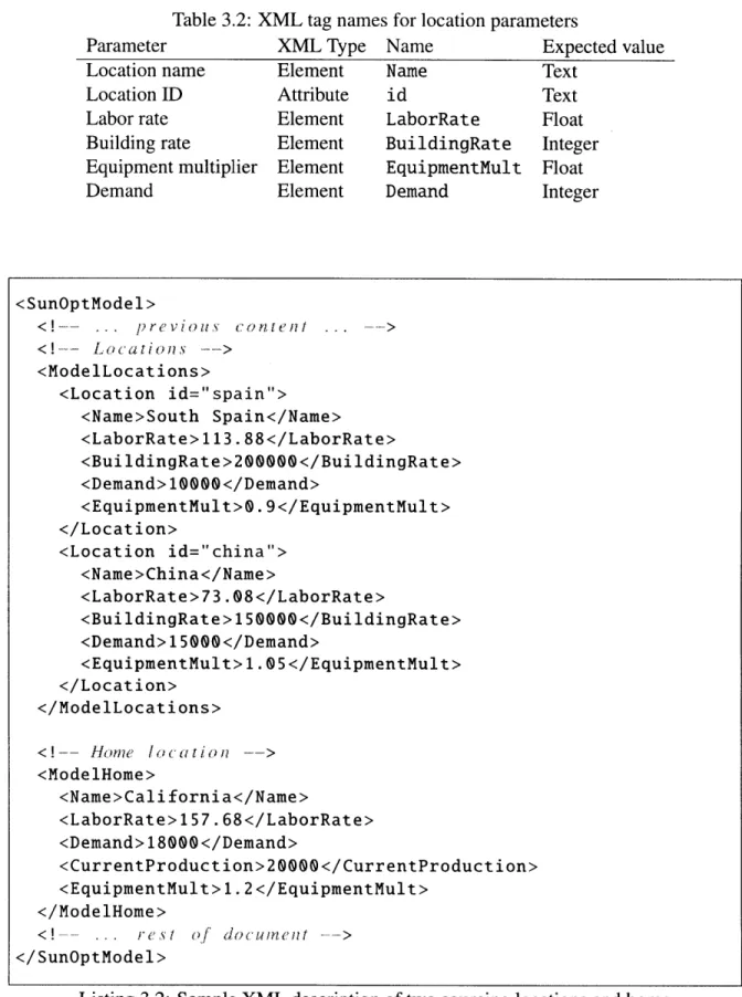
3.2 Sample XML description of two sourcing locations and home
3.3 Material cost table for two locations and four components . . . 3.4 XML file segment describing transportation rates . . . .
3.5 Part of XML file describing scenario for Panel . . . .
3.6 Python code for binning algorithm . . . .
3.7 Python code for combining items . . . . 4.1 Running the optimizer with default parameters . . . . 4.2 Running modelCost and its corresponding output . . . .
6.1 Equipment rate function as defined in tools. py . . . .
6.2 Example labor head cost function . . . . 6.3 Scenario cost calculation . . . . 6.4 Editing substrategy cost function for static/dynamic drivers . .
6.5 XML tree example with labor head . . . .
6.6 Reading locations from file . . . . 6.7 Using modelOptimize within Python . . . .
6.8 Using modelCost within Python .
. . . 41 . . . 46 . . . 48 . . . 50 . . . 51 . . . 54 . . . . 58 . . . . 59 . . . . 62 . . . 65 . . . 82 . . . . 82 . . . . 84 . . . . 85 . . . 85 . . . 86 . . . 88 . . . 89
Chapter 1
Background
1.1 Expansion alternatives
This project stemmed from a collaboration with Soliant,' a provider of concentrated solar energy systems. The project explores the expansion options available for a company like Soliant which currently has one factory producing its entire product supply.
In an expansion model, the modeler (user) is interested in determining the most cost-effective sourcing strategy for the company's product in order to meet global demand. Given multiple regions in the world under consideration for product marketing, the cen-tral question is whether it is more viable to expand current production in the existing fac-tory or create one or more new factories in the region or regions in question. Research by Aimee Constantine categorizes this expansion technique as "global manufacturing capacity model" [1].
There are several ways for a company to expand production in a global economy. One method is to expand manufacturing in the existing factory and establish distribution centers in the regions with demand. Constantine describes this technique as "single-site material flow cost". At the other extreme, individual factories are created in each of the regions in question. In this project, the resulting expansion cost lies anywhere in between these two.
1.2 Discrete nature
One of the greatest difficulties that arises when attempting an analytical solution to the expansion problem is the discrete nature of the problem itself, particularly regarding factory sizes. Factories are built according to a prototypical factory size which produces n total units of the product. Thus, if 10, 000 units are to be produced, then it would take 2 factories that produce 5, 000 units each, but it would take 4 with a production of 3, 000 in order to meet (and exceed) demand.
In addition to factories, certain cost drivers may be discrete in nature, perhaps having piece-wise linear cost functions which jump or change slope with production volume due to economies of scale, for example. All these nuances make optimizing a sourcing model nearly impossible with traditional methods like linear programming. While linear program-ming is generally well suited and efficient for optimization problems, existing commerical solvers are often too expensive or complicated to use with this model. For these reasons, a full-combinatorial computer program is proposed which offers several advantages over more specialized algorithms, including
" modularity: model parameters can be altered and extended as needed; " flexibility: default parameter values are included;
e portability: software runs on all platforms;
" accessibility: users need not be well versed in a specific computational field, as all
calculations are reduced to simple arithmetic; and
" stability: programs are based on stable and not transient software standards.
1.3 Recursive nature
The expansion model discussed in this project also features a recursive description of the bill of materials, which is best represented as a tree with multiple levels. Addressing the layered complexity of the bill of materials is a natural step for computer algorithms which are coded using the object-oriented programming (OOP) paradigm.
that are consistent with the layered structure of the assembly under consideration.2
1.4 Nomenclature
In this thesis, the following nomenclature is used:
Assembly the complete product to be manufactured, which is composed of subcompo-nents.
Subcomponent any part of an assembly or subassembly, as described in the bill of
mate-rials, which is to be manufactured.
Location a place under consideration for building a new factory in which to manufacture the assembly or any of its subassemblies and subcomponents.
Home a special location which currently has production and can expand to accommodate
new demand in several other regions. Consistent with the notion of an expansion simulation, the model assumes the existence of a current location, labeled home.
Region a geographic area for which there is demand for the final product (the assembly).
In particular, every location also represents a region. This assumption implies that factory expansion will be considered only in regions that have demand. This can be changed programmatically by setting the demand for a particular region to zero (see Section 3.1).
Cost driver any element that contributes to the net cost of manufacturing and supplying the assembly in any given location. Cost drivers include material costs, shipping
costs, labor costs, and others as discussed in Section 1.5.
Model parameters the collection of components (bill of materials), locations, and cost
drivers to be optimized, as described in the model file.
2"Flat" assemblies can also be studied with the programs by implementing a bill of materials consisting
Demand the expected number of units per year of the final product that will be marketed or
sold in a given region. This differs slightly in meaning from the traditional definition of demand. In practice, a given region's full demand might not be met by production intentionally for economical reasons. Since a region's demand is specified in the model, it is up to the user to adjust the value accordingly so that it indicates the number of units to be manufactured and sold.
Factory the building in which manufacturing takes place. Each factory that is built is assumed to follow a prescribed size known as the prototypical factory size, which is specified in the model. Such a size is reported in total number of units of final product that can be manufactured in such a factory. Every factory is capable of producing the entire bill of materials. It is possible, however, that a given factory is equipped to produce only a selection of the components in the bill of materials.
In addition to these parameters, the result of the optimization is organized according to the following terminology:
Source a location where some amount of one or more components are manufactured and shipped.
Destination a region receiving one or more components from any given source. Since
each location is also a region with demand, a source can supply itself, in which case
it is also a destination.
Strategy the set of sources and their corresponding destinations for any given component in the assembly, including the assembly itself.
Scenario the set of strategies for all the components in the bill of materials. This is the output of interest for a given model.
1.5
Cost
drivers
There are seven cost drivers included in the model cost function. Section 6.1 demonstrates how new cost drivers may be implemented:
Building costs are associated with building one or more prototypical factories. Any
loca-tion can build a discrete number of factories of the same size, as prescribed in the model. Creating multiple factories of the same size rather than single factories of different capacity is consistent with practice, enabling a company to work out the logistics of one prototypical unit and multiply accordingly.
Material costs are associated with the cost of the raw natural resources that go into pro-ducing any one component. These cost functions tend to vary dramatically from component to component and location to location.
Expansion and new line costs are fixed, one-time costs associated with either expanding
production of a given component (in a location where there is already production) or establishing a new line for that component in the given location. In particular, the home location always expands production while new factories incur a new line cost instead. These cost drivers are generally mutually exclusive.
Labor costs are associated with human capital and vary consistently across different
com-ponents depending on their manufacturing complexity. In addition, labor costs vary from location to location according to regional law and economics.
Equipment costs are one-time, fixed costs associated with stocking a factory with the necessary equipment to manufacture any given component.
Shipping costs are highly non-linear transportation costs associated with sending an
as-sembly/subassembly from a source to a destination. Because shipping costs tend to vary unexpectedly, they are specified as rates from any one location to any other
(including itself).
Carrying costs are the cost of holding pipeline inventory, and account for the total amount of goods that is neither in production nor at the destination region, but in transport.
Each of these cost drivers can be ignored if necessary in any given model, as the model can assume default values as discussed in Section 4.1.1. This feature is meant to provide
flexibility to the end user and speed up model creation without having to supply an exhaus-tive list of parameters.
1.6 Assumed utilization rate
Throughout this project, the utilization rate for all cost drivers is assumed to be 100%. Rather than carrying the utilization rate as a separate model parameter, the user is expected to supply the correct adjusted value assuming full utilization. When simulating a new factory being built, the assumption is that it will be utilized to its maximum potential. Deviations from 100% utilization rate only apply when testing the cost-sensitivity of the solution. This is done at a later stage in the decision making process not covered in this project.
The implications of 100% utilization is that fixed costs like equipment cost are calcu-lated similar to variable costs,
c = r - (qn) = rn, (1.1)
where c is the cost, r is the rate per component, n is the total number of components, and q = 1 is the utilization rate.
1.7 Constraints and assumptions
In order to reduce the parameter space and maintain simplicity, a number of assumptions and constraints have been placed on the algorithm, namely:
* Each region is sourced by only one location. This means that at no point in the sourcing strategy will one region receive the same (sub)component from two or more different factory locations. This assumption is consistent with the logic behind build-ing factories. Although in practice companies may need to complement a temporary change in demand in a region with supply from multiple sourcing locations, these unexpected changes in sourcing strategy occur on an ad hoc basis and are the subject of operation and not expansion models.
" Each region is also a potential location in which to build a factory. This assumption
blurs the definitions for the purposes of simplicity, since the program need not be aware of the true geographic distribution of the demand or the factories. There are, however, ways around this requirement, such as including a demand of zero for a given region. Doing so can simulate a possible factory location that is not also a
region, but the optimal solution will require some post-processing.
* As stated above, this model simulates expansion of product manufacturing. As such, it requires that there exist a special location labeled home, as mentioned in Sec-tion 1.4, which has current producSec-tion of the final assembly. ProducSec-tion increases in this factory location incur expansion costs instead of new line costs. By defini-tion, home currently produces the entire bill of materials, and is therefore always implicitly available for more production.
These constraints and assumptions are applicable to the client user for whom this code was designed, but may not be accurate for every optimization strategy. For such applica-tions, the results of the optimization algorithm could fail to identify the true optimal sourc-ing scenario. However, the strength of the program resides not just in its ability to produce an answer, but also its utility in testing sensitivities around a given answer. In addition, the program is structured so that it can be altered if necessary: adding or removing constraints as required by the end user. It is released as open-source under the GNU General Public License, as mentioned in Appendix B.1.
Chapter 2
Proposed Solution
This chapter details the proposed solution for solving the supply chain problem. The solu-tion maxim is divide-and-conquer. A number of relatively small computer scripts operate independently to fulfill their own single functional requirement. Together, they can be used to tackle a larger task by breaking the problem down into smaller, more manageable pieces. As will be shown, this solution approach is much more versatile than writing a single pro-gram to do it all. In addition, a greater number of case studies are available for analysis.
The two main sub-programs proposed are:
modelCost a program to find the cost of a given sourcing scenario based on model param-eters,
modelOptimize a program to generate all the viable scenarios recursively through the bill of materials and determine the best overall strategy using modelCost.
The first program, modelCost, provides a standard mechanism for calculating the sce-nario cost. Because the instructions in finding costs include simple arithmetic and negligi-ble decision-making, modelCost is a very fast program.
The work-horse of the solution is modelOptimize, a program which recursively tra-verses the bill of materials of the assembly, generating at each stage a set of possible sourc-ing scenarios, before ultimately outputtsourc-ing the most cost-effective one.
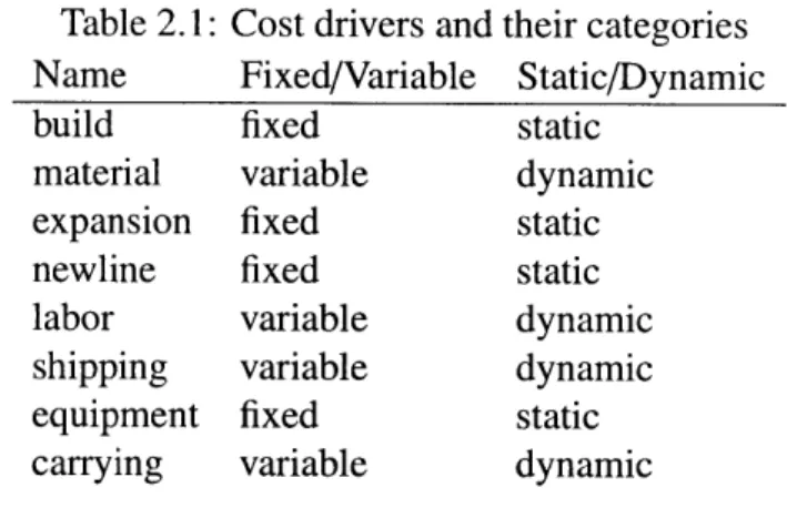
Table 2.1: Cost drivers and their categories Name Fixed/Variable Static/Dynamic
build fixed static
material variable dynamic expansion fixed static
newline fixed static
labor variable dynamic
shipping variable dynamic equipment fixed static carrying variable dynamic
2.1
Cost drivers
As discussed in Chapter 1, the objective function, z, is
z = building + material + expansion+
(2.1)
labor + shipping + equipment + carrying
The objective function must be minimized for the total cost due to production volume and factory lifespan.
Each of these costs can be described in two ways. The first way is fixed or variable depending on how the cost varies by production volume. The second way describes how each of these costs varies with time. Static costs are one-time expenses, such as building a factory. Time-varying or dynamic costs increase with the number of years. For the purposes of this project, the relationship between length of time and dynamic costs is linear, although non-linear relationships can be piece-wise approximated. The costs are organized in these categories in Table 2.1.
2.1.1 Direct and indirect costs
With the exception of building costs, all other cost drivers are direct costs: they are scaled
by the number of components produced. Conversations with client users revealed a greater
need for direct costs, and such is the focus of this project. However, indirect costs can be accounted for by lumping them into the building costs, or implementing a new cost driver
altogether, as discussed in Section 6.1.
The first method is easier, but altering the building rate may not reflect the true nature of certain indirect costs. In addition, when viewing the detailed log of the costs for a given scenario (see Section 4.2.1), the indirect costs will be hidden within the building cost. If finer control over indirect costs is required, then the second solution, implementing a new cost driver, is recommended. However, it is often enough to burden an existing cost factor in order to account for a new one.
2.2
Calculating costs
In general, costs are calculated using a function,
f,
linear in the number of components, n, and the rate, r, in $/component:dstatic = f(x) = nr, (2.2a)
where d represents one of the cost drivers. For dynamic costs, the cost function g is also scaled by the time horizon, t, to give
ddynamic = g(x) = nrt, (2.2b)
The total number of components is taken from the bill of materials and the specified number per assembly (see Section 3.1.1). The rate, r, for a given cost driver is determined in one of two ways. Where cost variation is the same across all locations or components, rate-multipliers are used. Where finer detail is required, look-up tables are used instead.
2.2.1
Rates and multipliers
As an example of a rate-multiplier cost calculation, consider the equipment cost driver. Like most other cost drivers, equipment costs vary from location to location and component to component. The larger variation is in the latter, so an equipment rate is assigned to each component. Such a rate is specified in $/component.
To reflect that one location is relatively more expensive than another, an equipment rate
multiplier is assigned to each location. These multipliers are normalized, so a location with
a multiplier, m, of 1.2 is 20% more costly than the standard, usually home. Using these two parameters, equipment cost for Component 1 in Location A can be found as
dequip = (nr), mA. (2.3)
Since equipment costs are static, there is no need to account for time horizon.
An assumption of the rates-and-multipliers method is that costs vary in the same fashion across the component or location with the multiplier. In the example above, the relative cost from component to component is the same across all locations: if one component is ten times more expensive than another in one location, it remains ten times more expensive in any other location. This approximation is valid for some costs like equipment, but is much too simple for non-linear cost drivers like transportation and material cost.
2.2.2
Look-up tables
Look-up tables allow utmost control in modeling the relationship between cost driver, com-ponent, and location. This is necessary for drivers like material cost because the relative costs of materials differs profoundly from one location to another. For instance, Location A might have a greater electronics infrastructure in place but poorer casting capabilities than
Location B. In this case, electronic-related materials are cheaper than casting-related
mate-rials in the Location A, while the relative costs are reversed in Location B.
A look-up table addresses this non-linearity by specifying a cost rate for each
component-location interaction. For the transportation costs, the rates to and from each component-location must be tabulated. The disadvantage of this method is its exhaustive nature: if there are A loca-tions, then there are C(A, 2), or n choose r, costs to determine and specify. Unlike rate-and-multiplier, look-up tables require full knowledge of the cost distribution. For this reason, they are only used where absolutely necessary for the sake of accuracy.
The rates found in the look-up table are then used to determine the net cost according to Eq. 2.2.
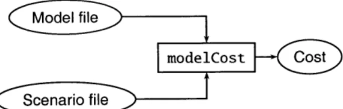
Figure 2-1: Input/output diagram for modelCost
2.3 modelCost
The first program, modelCost, calculates the net cost of a given scenario by using the model parameters. In particular, it solves the objective function, Eq. 2.1, by calculating the cost for each component in turn and then totaling it to yield the net scenario cost. The inputs and output of modelCost are shown diagrammatically in Figure 2-1.
For each component, modelCost determines the cost of each strategy (see Section 1.4). This entails the following steps:
1. If there is production in the location to source from (as is the case for home), then
calculate the expansion cost using the component's expansion cost rate times the
total number of units of component, dex = rn. For instance, if the number of units
of component to build is n = 2000, and the expansion rate for that component is
r = 1.50, then the expansion cost is dex = 3000. If there is no production, then determine the cost of establishing a new line. This cost driver function is similar to expansion cost.
2. Determine the material cost. This requieres using the look-up table for material cost to determine the rate for that component in the given manufacturing location, and scaling by the total number of units to be manufactured as specified by the demand.
3. Determine the transportation cost by using the transportation rate look-up table,
and scaling by the total number of units to be shipped to the destination.
4. Determine the labor cost by multiplying the labor rate for the manufacturing loca-tion times the labor rate multiplier for the component, scaled by the total number of units to be manufactured. For instance, if the labor rate for Location A is r, = 2.5
($/component), and the multiplier for that component is m = 2, then the labor cost
for manufacturing n = 1000 units is d, = n(rm) = 5000.
5. Determine the equipment cost similarly to the labor cost, using the equipment rate for the given component, and the equipment rate multiplier associated with the man-ufacturing location.
6. Determine the carrying cost as a percentage of the shipping rate specified by the
carrying rate parameter of the model, scaled by the duration of the transportation from one location to another, as specified in the transportation look-up table. This means that if n = 10, 000 components are being shipped from one location to another
on a trip that lasts J = 3 days, at a carrying rate of 10%, then the associated carrying
cost would total dcarr = 0.1 - n6 = 3000.
7. Determine the necessary number of factories to build and the associated building
costs by multiplying the location's building rate with the discrete number of factories required to supply the demand from all the regions to be supplied by the fractory in the location in question.
dbnild =
- r
(2.4)
FS
For instance, if the prototypical factory size, FS, is 4000 units, and the demand, s, for a given manufacturing location is 13000 units at a rate, r = 1.3, then the building
cost is $ 5200.
It is understood that each factory is of the same size (see Section 1.4). The total number of prototypical factories to be built in a given location is enough to at least meet the volume required for all the components to be built there. As an example, if the volume of Component A requires two prototypical factories, while the volume
of Component B demands three, then the building costs are those associated with
building three factories.
8. Other fixed and variable costs are factored into the total if specified for the given
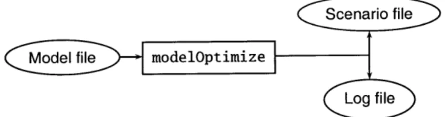
Figure 2-2: Input/output diagram for modelOptimize
At this point, the costs reflect the fixed vs. variable nature of the cost drivers, but assume a time horizon of one year. To determine the cost prorated for a given time span, the program scales each of the costs depending on whether they are static or dynamic (see Table 2.1),
" for static costs, prorated amount is the one-year cost divided by the number of years
(hyperbolic relationship dy = d/t),
" for dynamic costs, the prorated amount is the same as the single-year cost.
The program adds up the cost of each strategy (one for each component), to determine the net scenario cost. An example calculation of a scenario is detailed in Section 4.5.
2.4 modelOptimize
The main objective is to find an optimal sourcing scenario. To do this, modelOptimize takes in an input file describing the model parameters and determines the "best" scenario within the constraints. These constraints are necessary to reduce the solution space to a more manageable set and is intended to reflect the needs of particular clients. The most important of these constraints is the recursive step:
Optimization proceeds top-bottom through the bill of materials. Each com-ponent is independently optimized, and the resulting scenario appended to the existing scenario for all the components higher in the assembly.
This constraint indicates that no assembly's subcomponent can affect the optimal sce-nario for that assembly.
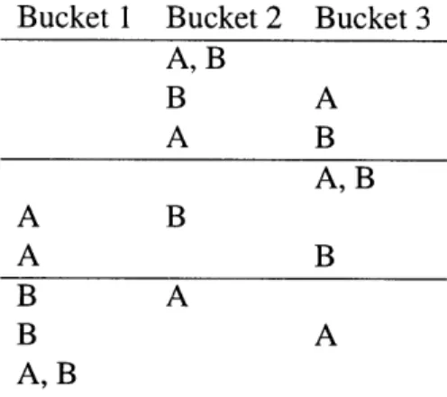
Table 2.2: Binning two items in three buckets, equivalent to assigning two regions to three manufacturing locations
Bucket 1 Bucket 2 Bucket 3 A, B B A A B A, B A B A B B A B A A, B
2.4.1
Program flow
The first step in finding the optimal scenario is to read the model parameters from the input file. After this initial setup process, modelOptimize starts with the root component of the assembly, and a list of all the potential locations.
Assigning production of a given component among a set of possible manufacturing locations to supply a number of regions can be described as a binning or bucket-filling problem. Each manufacturing site is represented as a bucket with unlimited capacity. That bucket must contain enough units of the component to supply any number of the regions. In a given scenario, any number of buckets can be empty, but at least one bucket must be filled as all the demand must be met.
In addition, a region's demand can only be supplied by one location as stated in Sec-tion 1.7. Therefore, only entire regions can be dumped into buckets. As an example, suppose that there are two regions to be distributed among three potential manufacturing locations (buckets). Table 2.2 shows the result of the binning problem. Each row in the table represents a sourcing strategy. The first row, for instance, has Buckets 1 and 3 empty, while the two regions (A, B) are dumped into the second bucket. This corresponds to a strategy in which Locations 1 and 3 are idle and factories are built as necessary in Loca-tion 2 in order to supply Regions A and B.
For b manufacturing buckets and A demand locations, the total number of different scenarios is n, = b. Because modelOptimize treats every region with demand as a
possible manufacturing location, the number of scenarios to inspect grows as n, - (A + 1)",
where the extra bucket represents the home location which can expand production yet has no demand.
After finding all the different possible strategies, the modelOptimize iterates through each one evaluating its cost via the procedure establised in modelCost. The program keeps the cheapest scenario at every level of the bill of materials. This scenario becomes the basis for the lower levels in the bill of materials, as the program recursively traverses the tree.
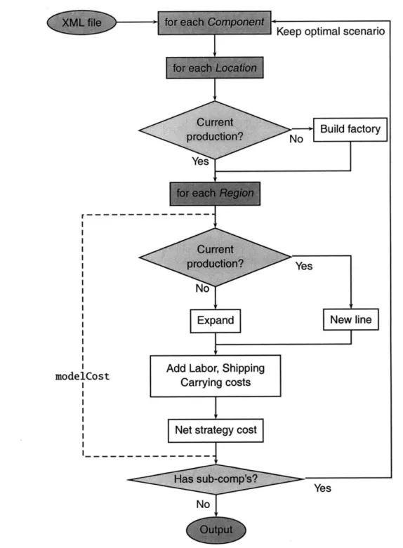
This workflow is shown diagrammatically in Figure 2-3.
2.5
Algorithm efficiency
Full-combinatorial algorithms tend to be slow. Even at - 0 (A), modelOptimize is very fast, considering its intended application. Usually, the user is interested in a handful of sourcing locations and a limited view of the bill of materials. For a typical number (A ~ 3) of locations and (c ~~ 6) components, the number of scenarios to consider is still within five
thousand.
On an Intel Pentium 4 processor with 2.8 GHz clock speed, such optimizations aver-age less than half a second, including model loading, optimization, and output. Even large assemblies, with ten components in six possible locations, take an average of 12 ± 0.3 sec-onds.
Most of the time, modelOptimize is run within other scripts using a relatively simple model, in order to test parameter sensitivity. Under these conditions, a case study with hundreds of data points would delay no more than a few minutes, making it ideal for quickly testing various situations.
ISince modelCost reads a model to file, modelOptimize does not call modelCost but simply executes its code with the model file already loaded in memory. This was implemented for performance reasons. See Section 6.2 for a discussion on this procedure.
Keep optimal scenario
production?' Yes
No
Expand New line
Add Labor, Shipping Carrying costs
Net strategy cost
Yes No
Figure 2-3: Flowchart for optimization function. After reading model parameters from XML file, step through the root component in the bill of materials: for each location de-termine the net costs due to supplying each region dede-termined from the binning algorithm. Repeat recursively with the subcomponents, keeping track of the optimal overall scenario.
2.6 Python as programming language
Python [4] is the programming language used to develop (and run) the programs. Python offers several advantages over other languages and platforms such as MATLAB [5], C++ and Java [6]. Table 2.3 compares four programming languages over five different criteria:
Development effort refers to the amount of time and effort from the programmer's
per-spective required to write and test the program. Compiled languages like Java and
C++ typically require longer development times because of the write-compile-test
cycle absent in dynamically-typed languages like Python. Once the MATLAB en-gine is running, execution of m-files is relatively quick.
Syntax complexity deals with the quirks of the language. Since these programs are meant
to be distributed in source form to the end user, who is not necessarily a computer scientist, it is necessary that the code be as straightforward as possible to facilitate debugging and program extension. A high score in this criterion reflects an easier syntax.
Accessibility refers to the relative costs (monetary, hard-drive space, installation, etc) re-quired to run each program or platform. Compilers for C++ are almost always in-stalled by default on machines regardless of operating system. MATLAB requires installation of the MathWorks's program and its costs2. Python and Java both
re-quire installing an interpreter and a virtual machine, respectively, but both of these are available free of charge for most operating systems.
User interface refers to how the user interacts with the program. Java and MATLAB
of-fer flexibility in developing graphical user interfaces (GUI), but since the programs are meant to be deployed multiple times and in batch scripts, graphical user inter-faces tend to be slow and cumbersome and therefore undesirable. Instead, a robust command-line user interface (CLI) is preferred, where Python and C++ thrive (see Section 2.8).
2
Table 2.3: Comparison of Python to other program platforms Python MATLAB Java C++
Development effort + + -
-Syntax complexity + + 0
-Accessibility 0 - 0
-User interface + 0 - +
Running speed 0 - - +
Running speed is imperative since the programs have to be run repeatedly in order to test sensitivities and gather useful data. MATLAB and Java (the former being dependent on the latter) both have a high start-up delay. For difficult number crunching, C++ is a clear winner in this category.
As shown in Table 2.3, Python comes out on top as the programming language of choice due to development and debugging facilities, relative speed of execution and accessibility. In general, it has been found that scripting languages like Python are easier to develop and are often more memory efficient than Java without being much worse than C++ [7]. All the programs discussed in this document are written in Python.
2.7
XML file format
The programs need to read the model parameters from a computer file. In addition, model-Optimize needs to write the optimal scenario to file, so that modelCost can use it to calculate costs (see Figure 2-1). A sensitivity analysis can be comprised of several dozens of these files each describing a slightly different scenario or a slightly different model. The Extensible Markup Language, or XML, was chosen as the format for these files because it is accessible, human- and machine-readable, and well supported and documented. XML is
documented at http: //www .w3. org/XML.
2.7.1 Basic description
XML is a markup language similar to its world-wide web sibling the Hypertext Markup Language (HTML). It is relatively easy to use and implement and has the advantage of
< ! -- (oini t -- >
<BuildingRate unit="USD">5000</BuildingRate>
Listing 2.1: Sample XML line
<Location id="spain"> <Name>South Spain</Name> <LaborRate>113.88</LaborRate> <BuildingRate>200969</BuildingRate> <Demand>1@@@@</Demand> <EquipmentMult>0.9</EquipmentMult> </Location>
Listing 2.2: XML tree example
being easy to read by both humans and machines. For example, Listing 2.1 shows a line from the file describing the model. In this case, it is clear that the value 5000 describes the
building rate. In the sample line, BuildingRate is called a tag.
In addition, Listing 2.1 also shows how to use comments. These are useful for the human reader. Note also the key-value pair: unit="USD". This is called an attribute of the tag. It is not uncommon to see an id attribute, which identifies the element represented by the tag throughout the document.
XML and tree structures
XML files are structured as trees of nested tags. A more complex example featuring this structure is shown in Listing 2.2.
The tags Name, LaborRate, and Demand are nested inside Location, indicating that they are descriptors of the location with id "spain". Adding a new location to the model would require duplicating the block and replacing its attribute and sub-tags with the appro-priate values.
Order neutrality
Another feature of XML is content order neutrality. This refers to the ability to place chil-dren of tags in any given order without confusing data. In the example XML file segment
shown in Listing 2.2, it is not necessary to specify the Name tag followed by the LaborRate. Any order of the five sub-tags would be equivalent, so long as they appear within the start
and end Location tags.
Related to order neutrality is white-space indifference. By default, XML ignores all white space, so the user is free to organize the document by adding indentation and empty lines where appropriate for clarity. Throughout this document, XML text will be shown with indentation that delineates the tree structure for readability.
2.7.2
Working with XML files
XML is plain text. Files written in XML can be edited using any text editor. In addition to the syntax mentioned in Section 2.7.1, XML files have two other requirements in order to be valid:
XML declaration the first line of the file which declares the version used (1.0) and the
character encoding, usually UTF-8,
Root element one and only one element inside the tags of which the entire document is
maintained. In the case of the model file, the root element is SunOptModel.
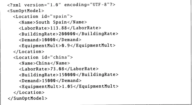
Using these concepts, a valid, though incomplete model file, is shown in Listing 2.3. XML files that are complete (well-written) can be viewed with most web browsers, which will usually render the tree structure using a collapsible interface and color coding3. A
common error when using an XML file is a missing closing tag for a given element. Using a web browser to view XML files will point out these syntax errors.
2.7.3 Comparison to other file format alternatives
Other ways to store file information are available. One alternative file format is tab-delimited, where each value-pair appears in a line separated by one TAB character or some other delimiter, such as a colon. Another method is to save the data as a binary format,
<?xml version="1.0" encoding="UTF-8"?> <SunOptModel> <Location id="spain"> <Name>South Spain</Name> <LaborRate>113.88</LaborRate> <BuildingRate>20000</BuildingRate> <Demand>1@@G0</Demand> <EquipmentMult>0.9</EquipmentMult> </Location> <Location id="china"> <Name>China</Name> <LaborRate>73.@8</LaborRate> <BuildingRate>150000</BuildingRate> <Demand>15@@G</Demand> <EquipmentMult>1. 5</EquipmentMult> </Location> </SunOptModel>
Listing 2.3: Valid XML file describing part of a model
Table 2.4: Summary of several file format alternatives XML Delimited Binary Tree structure + - 0 Human readable + + -Extensible + + 0 Cross-platform + - -Speed - 0 +
where each value-pair is saved using a special code that is hard-programmed into the soft-ware. This method has the disadvantage of being difficult to extend and impossible to use
by hand.
Table 2.4 compares the three main file formats in several different categories. Though slower (with larger file sizes), XML is the clear winner due to its flexibility.
2.8 Command line interface
An important part of the program interaction is the user interface. While information is transmitted by using files, there are several ways that the program can request values from the user and vice versa. The three main interfaces are graphical (GUI), command-line
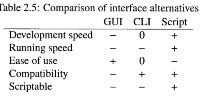
Table 2.5: Comparison of interface alternatives
GUI CLI Script
Development speed - 0 +
Running speed - - +
Ease of use + 0
-Compatibility - + +
Scriptable - - +
interactive (CLI), and batch script.
The last two are both types of command-line interfaces, but differ in that the former actively requests information from the user, while the latter only passively accepts options from the user. For instance, an interactive command-line interface prompts the user for the name of a file which describes the model. By contrast, a batch script interface requires that the filename be specified with the program call and runs (or fails) without interruption.
Running without stopping to prompt the user allows a program to be used inside other scripts. As will be shown in Chapter 5, it is often necessary to run modelCost several hun-dred times with slightly different model parameters. This is useful in sensitivity analysis.
If the program were to prompt each time for the model file, the user would have to actively
type hundreds of different file names if using an interactive interface.
Graphical user interfaces, though easier to use at first, are also encumbered by the need for active manipulation from the user. In addition, they tend to be much slower than their command-line equivalents because of the memory requirements of the graphical interface. Table 2.5 compares the three interface alternatives in five different categories. Due to its simplicity and scriptability, all the programs described in the proposed solution use the batch script interface.
2.8.1 Basic interface usage
To use the programs, open a shell in Unix systems, or the command prompt in Microsoft Windows. Assuming Python is installed and available, the programs can be run by entering their name preceded by the python executable4. Because every program described in this
41n
$ ./modelOptimize.py
Usage: modelOptimize.py [options] model.xml Options:
--version show program's version number and exit -h, --help show this help message and exit
--log=LOGFILE log activity in LOGFILE
-v be verbose: print log to screen -s SCENARIOFILE, --scenario=SCENARIOFILE
Usage: modelOptimize.py [options] model.xml modelOptimize.py: error: missing input model
Listing 2.4: Running a program from command line, with a brief usage message
$ ./mode10ptimize.py -- logfile=myLog.txt myModel.xml
Listing 2.5: Command with option and model filename
document requires at least one input, typing just the name of the program will output a brief usage message and a list of options, as shown in Listing 2.4.
As the message indicates, the program expects the name of a file which describes the model. To specify an option to the script, use the example shown in Listing 2.5.
Chapter 3
Model Details
This chapter discusses the full details of the programs' parameters. In addition, a number of example XML model files are provided and discussed. Sample scenario files will also be treated. Finally, some of the auxiliary functions are discussed along with their output.
3.1 Model parameters
The model used in the programs consists of the following inputs: " a bill of materials as a tree of components;
" a set of regions with demand for the final product (the root of the component tree); " a set of possible sourcing locations, which are considered to be the same as the
re-gions with demand;
" one home location where there already is production of the assembly, and which is capable of expanding production of any of the components;
" a table of material rates for each component in each location;
" a table of transportation rates from each location to every other, including home; " a prototypical factory size in terms of the total number of the components of the final
product that can be manufactured there;
" a carrying rate to account for inventory during shipping;
3.1.1
Bill of materials
The bill of materials (BOM) is a tree of the components to consider in the model. It can accommodate as many items as necessary, so long as each node in the tree has only one parent. Each node in the tree is a component. Every node except the leaf nodes are also
sub-assemblies. The root of the tree is the final product which is the main focus of the
supply chain; it is a special node also known as the assembly (Section 1.4). Each component is described in terms of the following parameters,
Name a descriptive title for the component, such as "Control Assembly."
Material an identifier code to be used in calculating material costs.
Expansion rate the rate in $/unit for expanding pre-existing production of the component at the home location.
New line rate the rate in $/unit for establishing a new production line for that component in any given location with no prior production.
Labor complexity a multiplier (see Section 2.2.1) that scales the labor cost for this com-ponent relative to others in the assembly.
Equipment rate the rate in $/unit for the cost of procuring the equipment required to manufacture the component.
Shipping rate multiplier a multiplier similar to labor complexity for scaling shipping costs relative to other components in the assembly.
Number per assembly the number of units of this component required to build its parent assembly, not the root assembly. For the root component, this value is 1.
Subcomponents the set of components which comprise this component's assembly, if ap-plicable.
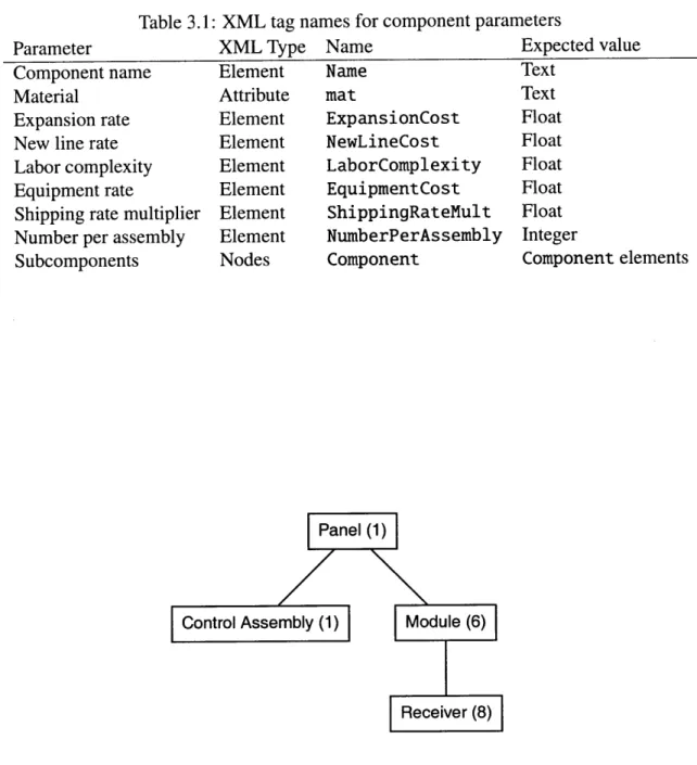
The XML element names for each of these component parameters are shown in Ta-ble 3.1. An example of a three-level bill of materials is shown as a diagram in Figure 3-1, and the equivalent XML representation in Listing 3.1.
Table 3.1: XML tag names for component parameters
Parameter XML Type Name Expected value
Component name Element Name Text
Material Attribute mat Text
Expansion rate Element ExpansionCost Float
New line rate Element NewLineCost Float
Labor complexity Element LaborComplexity Float
Equipment rate Element EquipmentCost Float
Shipping rate multiplier Element ShippingRateult Float Number per assembly Element NuberPerAssembly Integer
Subcomponents Nodes Component Component elements
Figure 3-1: Sample component tree. In parentheses is the number of components per parent assembly. In the case of the receiver, this implies that there are 6 - 8 = 48 receivers per panel.
<Component mat="panel"> <Name>Panel</Name> <ExpansionCost>1.2</ExpansionCost> <NewLineCost>1.2</NewLineCost> <NumberPerAssembly>1</NumberPerAssembly> <LaborComplexity>1.5</LaborComplexity> <EquipmentCost>2</EquipmentCost> <ShippingRateMult>1</ShippingRateMult> <! Secolnd level -- > <Component mat="control"> <Name>Control Assembly</Name> <ExpansionCost>1.4</ExpansionCost> <NewLineCost>1.4</NewLineCost> <NumberPerAssembly>1</NumberPerAssembly> <LaborComplexity>1</LaborComplexity> <EquipmentCost>2</EquipmentCost> <ShippingRateMult>&.7</ShippingRateMult> </Component> <Component mat="module"> <Name>Module</Name> <ExpansionCost>0.3</ExpansionCost> <NewLineCost>@.Q4</NewLineCost> <NumberPerAssembly>6</NumberPerAssembly> <LaborComplexity>&.05</LaborComplexity> <ShippingRateMult>0. 08</ShippingRateMult> <EquipmentCost>2</EquipmentCost> <!-- Third level -- > <Component mat="receiver"> <Name>Receiver</Name> <ExpansionCost>0.6</ExpansionCost> <NewLineCost>@.@8</NewLineCost> <NumberPerAssembly>8</NumberPerAssembly> <LaborComplexity>&. 6</LaborComplexity> <EquipmentCost>2</EquipmentCost> <ShippingRateMult>0. 05</ShippingRateMult> </Component> </Component> </Component>
XML tags for tree structure
As shown in Listing 3.1, each component of the assembly is contained within the Compo -nent tags. Subnents of a particular assembly are nested within the parent compo-nent's tag, as mentioned in Table 3.1. This architecture enables arbitrary assembly levels and complexity.
3.1.2 Manufacturing locations
The set of possible manufacturing locations excludes the home location. It is a list of new locations where one or more factories may be built in order to supply one or more regions. As mentioned in Section 1.4, a region with demand is also considered to be a potential sourcing location. Because of this, each model's location contains information about its potential to build the product as well as its regional demand:
ID an identifying code to be referenced throughout the model description,
Name a descriptive title for the location, such as "Southern Spain."
Labor rate cost in $/year/unit for a single worker in a region. This rate is later scaled by
the number of units of the component to be manufactured and the labor complexity (see Section 2.2.1) to determine the labor costs associated with one year of production of a given component.
Building rate the cost of building a new factory in the given location. Factory sizes are static and are provided in the model as a prototypical size. Building rate is the cost of building one factory of that size in the specified location.
Equipment multiplier a normalized scale factor used along with the component's
equip-ment rate (Section 3.1.1) and the total number of units to determine the cost of procur-ing the equipment necessary to manufacture the component.
Table 3.2: XML tag names for location parameters
Parameter XML Type Name Expected value
Location name Location ID Labor rate Building rate Equipment multiplier Demand Element Attribute Element Element Element Element Name id LaborRate BuildingRate EquipmentMult Demand Text Text Float Integer Float Integer <SunOptModel>
< -- ... pre viou s co nte . . > - Locations --- > <ModelLocations> <Location id="spain"> <Name>South Spain</Name> <LaborRate>113.88</LaborRate> <BuildingRate>200999</BuildingRate> <Demand>1@@@@</Demand> <EquipmentMult>0.9</EquipmentMult> </Location> <Location id="china"> <Name>China</Name> <LaborRate>73.@8</LaborRate> <BuildingRate>159090</BuildingRate> <Demand>15@@@</Demand> <EquipmentMult>1. 5</EquipmentMult> </Location> </ModelLocations> <!-- HomInle location -- > <ModelHome> <Name>California</Name> <LaborRate>157.68</LaborRate> <Demand>18@@@</Demand> <CurrentProduction>20000</CurrentProduction> <EquipmentMult>1.2</EquipmentMult> </ModelHome> <! - ... ,. re i of documein t > </SunOptModel>
The XML tags that describe a sourcing location along with their expected values are shown in Table 3.2. Part of an XML file that declares two sourcing locations is shown in Listing 3.2. All potential sourcing locations must appear in the file inside the Model-Locations tags, as shown. Like the Assembly element, model locations is a direct de-scendant of the root XML tag SunOptModel.
3.1.3
Home location
The special location with current production of the final product and its subcomponents is known as the home location and is described in similar terms as the sourcing locations, with one exception:
Current production the amount of the final product that is currently being manufactured
in the home location.
Although the home location is not a region to be supplied (it already supplies itself), a demand for home is still used in calculating the total number of units of the product that must be manufactured in order to supply itself and any other region. For instance, if the current production is 20000 units, and the demand is only 15000 units, then the home location need not build a new factory to supply a region with a demand less than 5000 units. Unlike the sourcing locations, the home location is contained within the ModelHome tag, which is a direct descendant of the root XML tag SunOptModel, as shown in List-ing 3.2.
3.1.4 Material cost table
As discussed in Section 2.2.2, material costs are calculated using a look-up table. Each component-location interaction is an entry in the table. Each entry consists of one XML element, Cost, with two attributes loc and mat which are the location ID and material, respectively, of the location and the component. The content of the XML element is a float value representing the cost per unit of the component in the specified location. The entire material cost table is contained within the tags MaterialCosts. This XML structure is