Analysis of a quadrotor in forward flight

Analysis of a

Quadrotor

in Forward Flight

ZU

.

9-by

James Neil Wiken

B.S., Aeronautical Engineering with Information Technology

Massachusetts Institute of Technology (2013)

Submitted to the Department of Aeronautics and Astronautics

in partial fulfillment of the requirements for the degree of

Masters of Science in Aeronautics and Astronautics

at the

MASSACHUSETTS INSTITUTE OF TECHNOLOGY

June 2015

@

Massachusetts Institute of Technology 2015. All rights reserved.

Auho....Signature

redacted"--A uthor

...

.. .

...

Department of Aeronautics and Astronautics

May 21, 2015

Certified by...Signature

redacted....

Jonathan P. How

Richard C. Maclaurin Professor of Aeronautics and Astronautics

Thesis Supervisor

Signature redacted

Accepted by ...

...

Paulo C. Lozano

Associate Professor of Aeronautics and Astronautics

Chairman, Department Committee on Graduate Theses

Analysis of a Quadrotor in Forward Flight

by

James Neil Wiken

Submitted to the Department of Aeronautics and Astronautics on May 21, 2015, in partial fulfillment of the

requirements for the degree of

Masters of Science in Aeronautics and Astronautics

Abstract

In general, quadrotors are designed to be stabilized about hover conditions. This allows the dynamics of the vehicle to be linearized about a single equilibrium point. Additionally, aerodynamic effects can be neglected leaving only rigid body dynamics to be modeled. While this formulation works under hover conditions, it is no longer valid when flying at high speed or in prolonged forward flight as the aerodynam-ics can no longer be ignored. This results in a highly nonlinear system with both

aerodynamics and rigid body dynamics affecting the dynamics.

In this thesis, a model of a quadrotor that takes into account both rigid-body dynamics and aerodynamics is presented. Flight testing was performed to test the validity of the this dynamic model. These flight tests were performed using a new flight space integrated into the Wright Brothers Wind Tunnel using a motion capture system. Additional flight tests were performed to gather data for a system identifi-cation of a quadrotor in forward flight using subspace methods. The results of the

system identification can be used for control design for the system. Thesis Supervisor: Jonathan P. How

Acknowledgments

First, I would like to thank my adviser, Professor Jonathan How. His patience and guidance have helped me through graduate school. He has an impressive ability of being able to get to the root a complex problem to find the solution.

I would also like to thank Professor Sheila Widnall for giving me the opportunity

to assist with teaching Dynamics. This was one of my most fulfilling opportunities while at MIT. Also thanks to Professor Julie Shah, her mentoring over the past five years has helped me during my entire MIT career.

I would also like to extend my gratitude to Richard Perdichizzi and David

Robert-son for their assistance with setting up, troubleshooting, and operating the new flight space added to the Wright Brothers Wind Tunnel.

Finally I would like to thank my all the members of the Aerospace Controls Lab-oratory. Much of what I have learned and accomplished over the past two years is because of those around me. In particular I would like to thank Mark Cutler for not only developing much of the hardware and software used to complete my research but to always be willing to answer any questions or help solve any problem I ran into. Also thanks to Brett Lopez, Byron Patterson, Justin Miller, John Quindlen, and Michael Klinker for assistance with flight testing and providing a sounding board to work through research problems.

This thesis is based upon work supported by the "Predictive Modeling in Uncertain Environments for Threat Assessment and Autonomous Driving" project under the Ford-MIT Alliance Agreement January 2008.

Contents

1 Introduction 13

1.1 Motivation . . . . 13

1.2 Literature Review . . . . 14

1.3 Contributions . . . . 15

2 Dynamics in Forward Flight 17 2.1 Rigid Body Dynamics . . . . 17

2.2 Aerodynamic Effects . . . . 20

2.2.1 Aerodynamic Drag . . . . 21

2.2.2 Induced Thrust . . . . 22

2.2.3 Blade Flapping . . . . 23

2.3 Equations of Motion . . . . 25

3 System Architecture and Control 27 3.1 System Architecture . . . . 27 3.2 Feedback Control . . . . 28 3.2.1 Position Control. . . . . 30 3.2.2 Attitude Control . . . . 34 3.3 System Dynamics . . . . 36 3.4 Simulation Results . . . . 37

3.4.1 Steady State Attitude Response . . . . 40

3.4.2 Actuation Limits . . . . 40

3.5 Summary . . . .

4 Flight Space

4.1 W ind Tunnel . .. . . . .

4.2 Camera Placement . . . . 4.3 Vehicle Setup . . . .

5 Hardware and Software Implementation 5.1 A ircraft . . . . 5.1.1 Physical Parameters . . . . 5.1.2 Aerodynamic Properties . . . . 5.2 Software . . . . 5.2.1 Outer Loop . . . . 5.2.2 Inner Loop . . . . 5.2.3 Data Logging . . . . 5.3 Sum m ary . . . . 6 Experimental Results 6.1 Experimental Design . . . .

6.2 Comparison of Physical and Simulated System

6.3 System Identification . . . . 6.4 Model for Quadrotor in Forward Flight . . . . 6.5 Summary . . . .

7 Conclusion

7.1 Sum m ary . . . .

7.2 Future Work ... ...

A Wright Brothers Wind Thnnel Flight Space Operation Manual A.1 System Setup ...

A.2 System Operation ...

46 47 48 49 51 55 . . . . 55 . . . . 55 . . . . 56 . . . . 58 . . . . 59 . . . . 60 . . . . 60 . . . . 60 63 . . . . 63 . . . . 64 . . . . 66 . . . . 69 . . . . 73 75 75 77 79 79 81

List of Figures

2-1 Free Body Diagram of a Quadrotor in Hover Conditions with Body Reference Frame B Centered at

Q

and Inertial Reference Frame I

Centered at 0 . . . . 18

2-2 Free Body Diagram of a Quadrotor in Forward Flight with Body Refer-ence Frame B Centered at

Q

and Inertial Reference Frame I Centered at0... ... 21

2-3 Blade Flap Angle of the Rotor Due to a Relative Wind [1] . . . .

24

3-1 Top Level Block Diagram of the Simulated System . . . . 28

3-2 Top Level Simulink Diagram of Simulated System . . . . 29

3-3 Simulink Diagrams of Blocks "positionController"; "positionController/ getAccel", and "positionControl/getAtt" . . . . 31

3-4 Simulink Diagram of Block "attitudeController". This Block Corre-sponds to the Attitude Control Loop (Inner Control Loop Described in Section 3.2.2 . . . . 35

3-5 Simulink Diagram of Block "equations of motion" Corresponds to the System Dynamics Described in Section 3.3 . . . . 38 3-6 Simulink Diagram of Block "equations of motion/6DOF (Quaternion)" 39 3-7 Steady State Pitch of the Simulated System as a Function of Wind Speed 41 3-8 System Response of Simulated Quadrotor Above Maximum Operating

Speed (32 mph). From Top to Bottom, The Plots Show Velocity in the Inertial Frame, Position in the Inertial Frame, Attitude in Euler Angles, and the Induced Thrust Forces All With Respect To Time. . 42

3-9 System Response of Simulated Quadrotor at Maximum Operating Speed

(30 mph) From Top to Bottom, The Plots Show Velocity in the Inertial

Frame, Position in the Inertial Frame, Attitude in Euler Angles, and

the Induced Thrust Forces All With Respect To Time. . . . . 43

3-10 System Response Time as a Function of Wind Speed . . . . 45

3-11 Tracking Reference Sine Wave in X-Position at 9 m/s (20 mph) . . . 45

4-1 Wright Brothers Wind Tunnel Flight Space with Vicon System . . . . 47

4-2 Wright Brothers Wind Tunnel Diagram [2] . . . . 48

4-3 Vicon Camera Placement in Wright Brothers Wind Tunnel . . . . 50

4-4 Flight Vehicle Size Reference . . . . 52

4-5 Example Vicon Dot Arrangement . . . . 53

5-1 The BuddyQuad, a Quadrotor Designed at the Aerospace Controls Lab 56 6-1 Steady State Pitch of the Simulated and Physical Systems as a Func-tion of W ind Speed . . . . 65

6-2 Model Output of Single State-Space System Identification Compared to Validation Data at 25 mph (11.2 m/s) . . . . 70

6-3 Model Output for Estimated Pitch Compared to Validation Data at 20 m ph (9 m /s) . . . . 73

6-4 Model Output of 4th Order, 4 Input State-Space System Identification Compared to Validation Data at 25 mph (11.2 m/s) . . . . 74

A-1 Wright Brothers Wind Tunnel Flight Space with Vicon System . . . . 80

A-2 Components of the Vicon system in the Wright Brothers Wind Tunnel 81 A-3 Network Setup for Flight Space . . . . 82

A-4 Vicon Camera Placement in Wright Brothers Wind Tunnel . . . . 83

A-5 Example Tripod Setup Within Test Section . . . . 84

A-6 Vicon System Calibration Tools . . . . 85

List of Tables

3.1 Rise and Settling Time of the Simulated System at High Speed . . . . 44

5.1 Physical Parameters of BuddyQuad . . . . 57 5.2 Aerodynamic Properties of BuddyQuad . . . . 59 6.1 Total Error of Model Output Compared to Validation Data . . . . 71

Chapter 1

Introduction

1.1

Motivation

Over the past decade or so, quadrotors have become an increasingly common type of aircraft in the field of unmanned aerial vehicles. They are used in an increas-ingly wide area of research topics ranging from forest fire observation [31 to package delivery[4]. As the range of quadrotor applications expands, so does the range of domains they must fly in, pushing into more extreme flight conditions. Recently, a particular interest in sustained high-speed quadrotor flight has increased [5].

High-speed flight, or forward flight, is an interesting regime for quadrotors as aerodynamic effects that are typically ignored when modeling these aircraft become increasingly important to the overall dynamics of the system as the speed of the air-craft increases. In forward flight, assumptions made about hover conditions, common in linear control techniques for quadrotors, become invalid as the aircraft is consis-tently operating at non-zero attitude conditions.

This thesis explores the difference in dynamics of a quadrotor when flying at high speeds compared to one operating about hover conditions. The dynamics model for the quadrotor must be augmented with aerodynamic effects which are commonly neglected in modeling multirotor aircraft. The aerodynamic effects govern the steady state response of the system when flying at a constant forward speed.

Flight tests were performed with a quadrotor in forward flight at nearly 30 mph. To perform these flight tests, a new flight space capable of supporting sustained high speed flight was developed.

1.2

Literature Review

Small quadrotors, first developed as recreational electronic aircraft, gained popularity as platforms for aerial control in the early 2000s [6]. In the past decade, they have become increasingly common as test aircraft for controls research. In addition to the mechanical simplicity and relatively low cost of the aircraft, low speed quadrotor flight is well understood and highly documented.

Early works in quadrotor flight and control often approximated the dynamics of the aircraft into a linear system [7]. This allowed the system to be controlled by a simple linear controller, often around hover conditions. More recently, nonlinear control techniques have been applied to nonlinear models of quadrotors [8]

191.

These models, however, neglect the aerodynamic effects acting on the vehicle which become relevant while flying at high speeds. When flying in demanding flight regimes such as these, the control performance can be diminished if the aerodynamic effects are neglected 1101. In these situations, the control signals could drive the system into the region of saturation causing undesirable or even unstable behavior. These effects are especially important to model when the quadrotor is flying near its operational limits

111].

More recently, there has been some work on incorporating aerodynamic effects into quadrotor models. [10] discusses the effects of blade flapping and induced thrust acting on a quadrotor. The behavior of a quadrotor propulsion system (with focus on its limitations) while in forward or descent flight is discussed in

[111.

A six

degree-of-freedom model incorporating blade flapping, induced thrust, and aerodynamic drag is presented in [1]. However, both [11] and [1] only provide simulation data based on their models.

[101

provides some experimental data to specifically model blade flapping, but is largely limited to test stand flights.

1.3

Contributions

The main contributions of this thesis are as follows:

1. A new flight space is constructed by augmenting a wind tunnel with a motion

capture system to allow for autonomous free flight at high forward speeds. Additionally, an operation manual for the flight space is provided.

2. The validity of a full dynamic model incorporating rigid body dynamics and aerodynamic effects is evaluated using flight test data.

3. Flight experiments are conducted to perform a system identification of a

quadro-tor in forward flight, providing estimated state-space models for the system at different flight speeds.

Chapter 2 provides the derivation of a dynamic model for a quadrotor in sustained forward flight. This model incorporates both the rigid-body dynamics commonly model in quadrotor dynamics and aerodynamic effects that become important when flying at high speed.

A system architecture including controller formulation is provided for the system

in Chapter 3. The control law presented is not based on near-hover conditions, which makes it usable for the flight regime being analyzed. Additionally, the full system is simulated using Simulink, the implementation of which is detailed. Steady state performance, operating limits, and control performance of the system are then discussed.

Chapter 4 details the design of the new flight space in the Wright Brothers Wind Tunnel. The properties and capabilities of the wind tunnel are briefly overviewed. The design and reasoning behind the camera placement is then discussed. Finally, vehicle setup and limitations while flying in the wind tunnel are provided.

The hardware and software implementation of the flight tests is detailed in Chapter

5. Included are tables of the physical and aerodynamic qualities of the test aircraft.

Experimental results from flight tests performed in the wind tunnel flight space are presented and analyzed in Chapter 6. The experimental design and challenges are discussed. A comparison of the simulated system from Chapter 3 and the per-formance of the physical system is discussed. A brief overview of subspace methods for system identification of state-space systems is given. The system identification process is described along with performance results of the final state-space model of the quadrotor in forward flight at various speeds.

Chapter 2

Dynamics in Forward Flight

In this chapter, the dynamics of a quadrotor in forward flight are derived. This model is complicated by the fact that a quadrotor flying at sustained high speeds is subject to both the high speed body dynamics (normally experienced by quadrotors in hover conditions) and the low speed aerodynamic effects more commonly seen in fixed-wing aircraft. This combination of effects results in a highly nonlinear set of equations of motion.

The chapter begins with a review of the rigid body dynamics used to model quadrotors at hover conditions in Section 2.1. Section 2.2 discusses the various aero-dynamic effects that a quadrotor experiences while operating in forward flight and how they are incorporated into the existing dynamic models. Finally, Section 2.3 is the complete equations of motion for a quadrotor in forward flight.

2.1

Rigid Body Dynamics

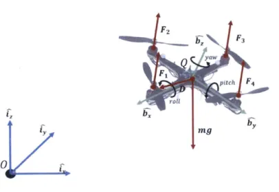
This section derives the equations of motion for a quadrotor in hover conditions. The free-body diagram shown in Figure 2-1 shows the forces acting on the quadrotor in hover conditions and the two reference frames used through the rest of the thesis. This includes the inertial reference frame I (centered at origin 0, unit vectors ix, iy, i,) and the body reference frame B (centered at origin

Q,

unit vectors b_, by, b,). Five forces act on the quadrotor in hover conditions: gravity and the four thrust forces.

0LI-F2z

F3

pitch F4

Mg by

Figure 2-1: Free Body Diagram of a Quadrotor in Hover Conditions with Body Ref-erence Frame B Centered at

Q

and Inertial Reference Frame I Centered at 0

The inertial orientation of the body frame is

sequence (yaw

(p),

pitch (0), then roll

(h)).

body frame to the inertial frame is

described using a 3-2-1 Euler angle The transformation matrix from the

RB = _c@s-} [-sO sOsOcO - cqsV/ S$SOS'i/ + cOcV4i s/c6 cOsOc4'

+

sds'1

c$SOS'

+

sc15'b

cc6

where cO and sO are abbreviations for cos 0 and sin 0, respectively. This also applies

for the other angles, 0 and V).

Derivation of the translational equations of motion starts with Newton's 2nd Law

F = md. (2.2)

As stated above, there are five forces acting on the aircraft: gravity (mg) and the four motor thrusts (F1, F2, F3, F4). Gravity always points purely in the negative iz

direction. The four thrust forces all point purely in the b2 direction. Using this knowledge and Equation 2.1, Newton's 2nd Law can be rewritten into translational

equations of motion for the quadrotor

0 0

m IRB [ B (2.3)

.- -Ft.a B - -g I

where Ftotal is the sum of the thrust forces, m is the mass of the aircraft, and

1T

I 2] is the second derivative of the position vector of the quadrotor in the

inertial frame (p)

p = XiX + Yy + ziz. (2.4)

The rotational equations of motion are derived from the rotational equivalent of Newton's 2nd Law

where T is a torque, I is the inertia tensor, and c is the time derivative of the angular velocity of the quadrotor body frame with respect to the inertial frame

w = pbx + qby + rbz. (2.5)

Note that rotation of the quadrotor is defined about its center of mass. Thus, torques are created from the quadrotor motion, the thrust forces, and the rotors spinning. Including these torques and rearranging gives the general form for the rotational equations of motion

4

I=-W X I + IZTk/cm x Tk.

+

L

x

IrQ

(2.6)

k=1

where I is the inertia tensor of the quadrotor, 1, is the inertia tensor of the rotor, and

rk/cm is the distance between the kth rotor and the center of mass of the quadrotor.

other words, their inertia tensors are diagonal matrices

Ix 0 0

0 I 0 (2.7)

0 0 Iz

Rotor inertia tensors exhibit the same property. The rotational equations of motion are

I4 = -(Iz - I,)qr + L(F3 - F4) (2.8)

IA = -(Ix - Iz)rp + L(F2 - F1) (2.9)

4

Izr = -(I, - Ix)pq + cm F (2.10)

k=1

where L is the distance from the rotor to the center of mass of the quadrotor (arm length) and cm is a constant relating the thrust force and the yawing moment caused

by spinning the rotors.

2.2

Aerodynamic Effects

The following section discusses the aerodynamic effects that are taken into account for the dynamics model presented in Section 2.3. The model includes the effects of aerodynamic drag, induced thrust due to translational flight, and rotor blade flap-ping. A free body diagram including these effects is shown in Figure 2-2. Note the differences from Figure 2-1, namely the inclusion of a sixth force (D) corresponding to aerodynamic drag and the four thrust forces are tilted and now have components in the b, and by directions.

In aerodynamics, the velocity of the aircraft is often modeled as an apparent wind acting on the vehicle. The velocity of the vehicle in the body frame (v) is related to the relative wind velocity vector (Vrei) with the relationship

1z

0Ly

F2

F1

pitch F4

Figure 2-2: Free Body Diagram of a Quadrotor in Forward Flight with Body Reference Frame B Centered at

Q

and Inertial Reference Frame I Centered at 0

The relative wind velocity vector acting on the kth rotor is defined as

Vrelk = Ukb + Vkby +

Wkbz.

(2.12)

Similarly, the relative wind velocity vector acting on the center of imass is defined as

Vrel,cm = Ucmbx + vcmby

+

wcmbz. (2.13)

2.2.1

Aerodynamic Drag

The aerodynamic drag is modeled as acting on the center of mass of the vehicle. Thus no moments are created by the drag force. The drag force is defined as

D =WD IIrel,cm I2rel,cm (2.14)

where WD is a drag constant that incorporates the effects of the coefficient of drag (CD), density of air (p), and reference area (S),

1

WD = -PSCD.

Calculating the aerodynamic drag in the body frame has the added benefit that the reference area is constant no matter the orientation of the vehicle. Quadrotors tend to be symmetric about all three body axes, thus the drag constant is the same when flying in either direction along a body axis. The drag constant along each body axes can be unique such that

WD,x 0

0

WD 0 'D,y 0 (2.16)

0 ₀

'eD,Z-2.2.2

Induced Thrust

Relative wind velocity changes the magnitude of thrust generated by a rotor through two main effects. The first is an increase in thrust due to horizontal translation (induced thrust). The other is a decrease in thrust if the relative wind in the b, direction is negative. In short, the thrust from a rotor decreases in climb and increases in horizontal translation. To calculate the change in thrust due to these two effects

2

ki

k + (V, +W

Tk = Fkvik (2.18)

Vi,k + Wk

where vh _{is the induced velocity in hover (determined using momentum theory}

₁₁₁₁₎

and Fk is the commanded thrust (control input) [1]. Momentum theory states that for an actuator disk of area A with induced velocity vh, and with air density p, the mass flow rate h through the disk is

r =

pAvh-For a quadrotor in hover, the velocity far upstream of the actuator disk is zero and the velocity far downstream of the actuator disk is Wh. Conservation of momentum states that the total thrust T of the actuator disk is equal to the rate of change of

momentum

T = rnwh.

Conservation of energy states

1 2

T~ m2Twh.

Substituting in and solving for Vh

1

Vh = -Wh.

2

Using this value for Vh and the equation for rh

T = lWh = 2pAv .

Finally, solving for Vh

T

Vh 2Ap (2.19)

Equation 2.17 results in a fourth order polynomial when solving for the induced velocity. In climb (wk < 0), the equation has only one positive real root which corresponds to the physical solution [101. In hover (wk = 0) the induced velocity is Vh. In descent (wk > 0), the airflow through the rotor is steady, therefore the

momentum theory based solution listed above is not valid.

The main limitation of the model presented in equations 2.17 & 2.18 is that it only holds when wk > 0 or Wk > 2Ivkl [101. When wk is not in this range, the rotor is in Vortex Ring State, a region where the aerodynamics are unsteady and momentum theory breaks down. Generally, the solution is to fly quickly through this flight regime to avoid the dynamic instabilities that occur.

2.2.3

Blade Flapping

Figure 2-2 pictures the thrust vectors tilted away from the b. axis. This is due to rotor blade flapping. This effect occurs due to a difference in lift experienced on the advancing and retreating sides of the rotor while in translational flight. Specifically,

C k

bz

Tk

Vrelk

Figure 2-3: Blade Flap Angle of the Rotor Due to a Relative Wind [1]

due to the translational velocity of the vehicle, the advancing rotor blade observes a higher relative velocity than the retreating blade, and therefore produces more lift. This results in an aerodynamic load differential across the rotor, causing the blades to flap during rotation. The loading cycles of the rotor occur at the same frequency as its rotation. This causes a resonance that causes the maximum deflection of the blade to occur 90 degrees out of phase [12]. This results in the entire rotor disc tilting away from the apparent wind, deflecting the thrust force away from the b. axis.

Blade flapping is a function of the relative velocity in the x-y direction in the body frame. In sustained forward flight, the relative wind over each rotor is assumed to be equal. As such, the blade flap angle ak (see Figure 2.2.3 can be approximated as

a=k

'1L + V

(2.20)

where kf is a constant representing the relative displacement of a particular rotor

[1i.

The value of kf is the same for all four rotors (as they are assumed to be the same type of rotor). The actual value parameter kf must be determined experimentally, but can estimated given that blade flap angle tends to be on the order of one degree in moderate wind [10].

b. axis. Using geometry, the thrust vector of the kth rotor (Tk) is

Tk= Ti 1sin

ab,

+ V/csin aby

+ cos a)

(2.21) where Ti and ;k are the x and y components of the relative wind vector of the kth rotor normalized in the x-y body plane

Xk= Uk u~+ '11 V/c V/c (2.22) (2.23)

2.3

Equations of Motion

In this section, the equations of motion from Section 2.1 are augmented with the aero-dynamic effects described in Section 2.2. The resulting equations of motion describe the dynamics model used to simulate a quadrotor in forward flight.

From Equation 2.3, the general form for the translational dynamics is

rni

C1 0

=1RB C2 - 0

C3 B . - I

(2.24)

Note that the thrust forces now have components in the b, and by axes due to blade flapping. The equation for C1, C2, and C3 are

4

Ci = (rDeIVrel,cm Ucm

+ E/c

sin

a

Ti,k)

k=1

C2 = ((Dy Vre1'CM

Ucm

4 + ZV/ksin

a

Ti,k) k=1 4 C3 = ( ,_IVrel,cm I + c1os a k=1 Ti,k ) (2.25) (2.26) (2.27)

and the rotation matrix between the inertial and body frames (Equation 2.1) is

cOc< sOsOc4' - cOs'< cCOsOc't,

+ s/su/

IRB cOSV SSOS) +C cc c/s s -

S

sc+ c

--so sOcO cOcO

(2.28)

From Equation 2.6, the general form of the rotational dynamics is

(2.29)

1W = -w x I + rk/cm x Tk. + w x I42.

k=1

Augmenting the hover equation with the aerodynamic effects results in the following rotational equations of motion

4

I14 - - (I, - T.) qr - ZdTvksin a (Tk) + L cosca (T4 - T2)

IVq = -(IX - I,)rp - dLk sin a(Tk) + L cos a(T3 T1)

4

Ii -(It - Ix)pq - L siri ce (,PTi - '73T₃ + 71₄T4 - 'iU2T2) + cm

S

Fk

(2.30)

(2.31)

(2.32)

To simulate the system, the rotational kinematics for a 3-2-1 Euler angle sequence are used

=p

+

q sin 0 tan 9

+

r cos o tan 9

0

= q cos

#

- r sin

#

4'

= q sin 0 sec 0 + r cos 0 sec 0.

(2.33)

(2.34)

Chapter 3

System Architecture and Control

This chapter describes the system architecture and control algorithms used for the quadrotor in forward flight. The outer loop control algorithms described in this chapter are similar to those presented in [131. The attitude control law presented does not assume near hover flight regimes, making it a good fit for the application of sustained forward flight.

First the overall system architecture is described followed by a discussion of the control algorithms employed to control a quadrotor flying at high speed. The full system was implemented using Simulink [141. Graphical implementations of the con-trol laws and equations of motion are provided throughout this chapter in the form of Simulink diagrams. Simulation results including equilibrium states and operating limits are discussed at the end of the chapter.

3.1

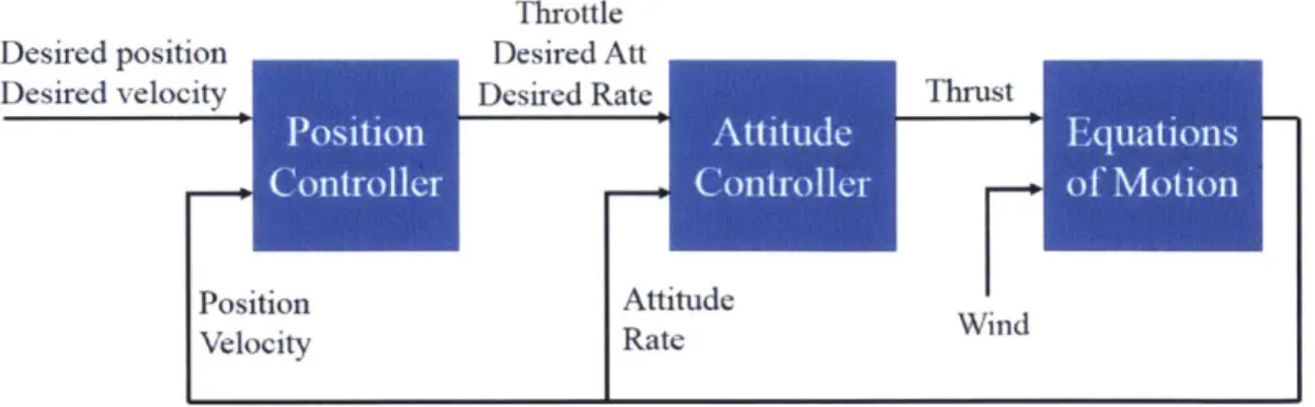
System Architecture

The system architecture is designed using two levels of successive loop closure. The outer most loop is position control loop. This loop takes as inputs a set of reference position and velocity along with measured position and velocity. It outputs a desired attitude, desired angular rate, and motor throttle command to be passed to the next level in. The inner control loop is an attitude controller. This loop takes as inputs the output of the position controller (desired attitude, angular rate, throttle command)

Throttle Desired position Desired Att Desired velocity Desired Rate

Position Attitude _Wn

Velocity Rate

Figure 3-1: Top Level Block Diagram of the Simulated System

along with measured values for the attitude and angular rate of the quadrotor. Motor commands, which are the outputs of this control loop, which are fed into the equations of motion described in Chapter 2 if simulating the system, or to actual motors if using hardware. The system dynamics take motor commands and wind speed as inputs arid output the measured values for position, velocity, attitude, and angular rate to be fed back to the inner arid outer control loops. Note that the implenenitation of the system presented in this chapter uses wind speed as a direct input into the system dynamics. This method was chosen because it most accurately matches the experimental set up using the wind tunnel to be presented in Chapter 4. Another Simulink diagram was implenented using a velocity controller as the outer control loop, commanding non-zero reference velocities, and eliminating wind speed as aii input into the system dynamics. The resulting behavior was identical to the presented system architecture, confirmiing that using a wind tunnel as a proxy for high speed flight does not change the dynamic response. A top level block diagramn of the system is shown in Figure

3-1 including inputs arid outputs of each block. Figure 3-2 is the top level view of the

Simulink model implementation of a quadrotor in sustained forward flight.

3.2

Feedback Control

This section describes the control algorithms used to stabilize a quadrotor in forward flight. The outer loop controller will first be described, followed by the inner loop

0 2

~I

cv V ,

~

t

I

I

-Figure 3-2: Top Level Simulirik Diagram of Simulated Systern 29

controller. Simulink implementations of both control loops are also provided. The system is controlled using two successive control loops which match the controller of the physical system described in Section 5.2. All positions, velocities, and attitudes used in the control loops are in the inertial frame I.

3.2.1

Position Control

The position control loop (also referred to as the outer control loop) takes as inputs the reference position and velocity and the measured position and velocity. The measured values are fed into the outer control loop from the system dynamics. The reference values are inputs into the system as a whole and can be set directly or through a trajectory generator. The position control loop is a two step process. First, desired accelerations are computed using the position and velocity inputs. The desired accelerations are then used to compute a motor throttle command and desired attitude and angular rate for the quadrotor.

To compute the desired acceleration vector, a position error vector (epos) and a velocity error vector (erate) are calculated

r

]T

F1T

epos [Xdes Ydes Zdes - [~ meas Ymeas zmeas] (3.1)

]T

T

ep

0 8 = [Xdes Ydes Zdesj me[meas ea measJ 32

where [xdes Ydes Zdes is the desired position vector, [meas Ymeas Zmeas T is

]T

T

the measured position vector, [des Pdes ides T is the desired velocity vector, and

I'meas O'meas imeas] is the measured velocity vector. The errors are mapped into

acceleration commands using a PID controller

T t

[Xcmd Ycmd Zcmd = Kpposepos + K1,pos0

]

epos + KD,posevel (3-3)

Sinulink Block "positionController" Corresponds to the Position

(Outer Control Loop) Described in Section 3.2.1

Control Loop

Siiulink Block "positionController/getAccel" Corresponds to the First Step of the

Outer Control Loop Described in Section 3.2.1

-1q R A a qq ) q1 Q 1r

Sl B

ositCntorm Qtatehieon

Co Prodeci oicat3on MulS

Fbar ProductC

2

Rotation Angles to Chuatemrions

2 yawdes Rakmm 0,11e, ZY x

Simulink Block "positionController/getAtt" Corresponds to the Second Step of the Outer Control Loop Described in Section 3.2.1

Figure 3-3: Simulink Diagrams of Blocks3'positionController", "positionController/ pos_des

Pspos

poe F - F m ooCoM

- vedes getMtoCthrotte

ttes q [R

yaw des : Quaternrdna to R01ation Anges K

getAtt R ato rdrZ

D-D

rateYw d rate des

1 , +- cs-efrr 7K-m s

pots-des _{Saturation Kp mass}

S

-K-por.

~

Integrator Ki + +

Sat~x F

Val

Gravity is then taken into account to compute the desired accelerations

T T

' des [ide des Yds Zes]T [cmd Ycmd ides = 1e

Zcmdl

Qm T +

[0

0 g](34cz (3.4)

To compute the motor throttle command (hcmd), the desired accelerations are turned into forces, summed, and mapped to a throttle command

hcmd = m( 'des + Ydes + des) (3.5)

kmotor

using an experimentally-determined motor constant (kmotor). The motor throttle command is then output to the inner control loop.

The second step of the outer control loop computes the desired attitude and angular rate given the desired accelerations. For this step, the attitude of the vehicle in the inertial frame is described by quaternion q and the angular rates in the body frame B defined as Qb. The quaternion q is defined as

q0

q=

q

where q0 is the scalar component and q is the vector component. The desired force vector in the inertial frame is defined as

F,des = m(adesix + Ydesiy + Zdesiz) (3.6)

and Fb,d.e _{is the desired force vector in the body frame. Equation 3.11 in [131 gives a}

relation between the desired attitude quaternion (qdes) and the desired force vector

S0

_d = qdes _ J qdes (3.7)

Fb,des-where Fb,de, and Fi,des _{are unit vectors,}

Fb,des = Fbes =

[0

0 1] (3.8)

|Fb,des|

Fi,des -Fi,de (3.9)

IIFi,desll

q*e is the quaternion conjugate of qde,, and 9 is the quaternion multiplication oper-ator. In this formulation, qde, corresponds to the quadrotor attitude (not including desired yaw) that aligns the body frame force vector with the inertial force vector. The minimum-angle quaternion rotation between the two force vectors in R3 is [151

qdes = _ .ideb:s (3.10)

2 i +Fdes Pb,des ) _ iesxY ae

Note that Equation 3.10 does not produce a unique desired attitude quaternion. In particular, quaternions define the special orthogonal group SO(3) in two ways. This results in q and -q defining the same attitude [13]. To remove this ambiguity, the sign of qdes is chosen to match the sign of qdes at the previous time step.

The desired attitude quaternion is then rotated by the desired yaw angle (Vaes)

to compute the full desired vehicle attitude quaternion

qdes,f = qdes 0 [Cos(i'des/2) 0 0 sin(Odes/2)]T (3.11)

In the Simulink implementation of the system, the desired attitude quaternion is converted into Euler angles and output to the inner control loop.

The desired angular rate (Qb,des) is calculated by taking the time derivative of

Fi,des. From

1131,

the angular rates in the x and y body axes is

where the time derivative of the inertial desired force vector is

F ,des Fi,des(Fides ides)

Fj,des -3 -3.1-

)

1F

i

,des

I

IFidesII

The z component of the angular velocity (yaw rate), is directly computed from the input yaw command

(Qb,des)z = des. (3.14)

The desired angular rate of the quadrotor is then output to the inner control loop. Figure 3-3 is the Simulink model for the position control loop. The figure includes a complete view of the outer control loop along with a detailed view on the first step, calculating a desired force vector from position and velocity (orange block), and the second step, calculating desired attitude, angular rate, and throttle command from the desired force vector (yellow block).

3.2.2

Attitude Control

The attitude control loop (also referred to as the inner control loop) takes as inputs desired attitude and angular rates from the outer control loop and measured attitude and angular rates from the system dynamics. Its purpose is to output motor com-mands to the system dynamics. First, an attitude error vector (eatt) and an angular rate error vector (erate) are calculated

eatt = [des Odes Odes T -

L0meas

0meas i)meas T (3.15)

- T T

erate [Pdes qdes rdes - [pmeas qmeas rmeasj

(3.16)

where [Odes Odes 'Odes] T is the desired attitude

vector[

$meas meas meas T is the measured attitude vector, [Pdes qdes rdes]T is the desired angular rate vector, and

m T t

I I + + IAI Figure 3-4: Simulink Diagrami of Block "attitudeController". This Block Corresponds to the Attitude Control Loop (Ininer Control Loop Described iii Sectioni 3.2.2 35

pitch, and yaw commands (qcmd, 0cmd, and 'cmd, respectively) using a PID controller

T t

[cmd Ocmd Ocmd T KPatteatt KI,att

j

eatt + KD,atterate (3.17)

where Kpatt, K,att, and KD,att are 3x3 diagonal, positive semi-definite gain matrices. The angle commands are then used with the motor throttle input (hcmd) to calculate motor commands

mi 1 0 -1 -1 hcmd

M2 1 -1 0 1 Ocmd (318)

M3 1 0 1 -1 9cmd

m4 1 1 0 1 cmd

In simulation, the motor commands are then converted to motor thrusts (F, F2,

F3, F4) in Newtons using an experimentally-determined motor constant (kmotor) and

then saturated to within the actuator limits

Fk = kmotormk. (3.19)

The thrust forces are then fed into the system dynamics as the outputs of this control loop. Figure 3-4 is the Simulink model for the attitude control loop.

3.3

System Dynamics

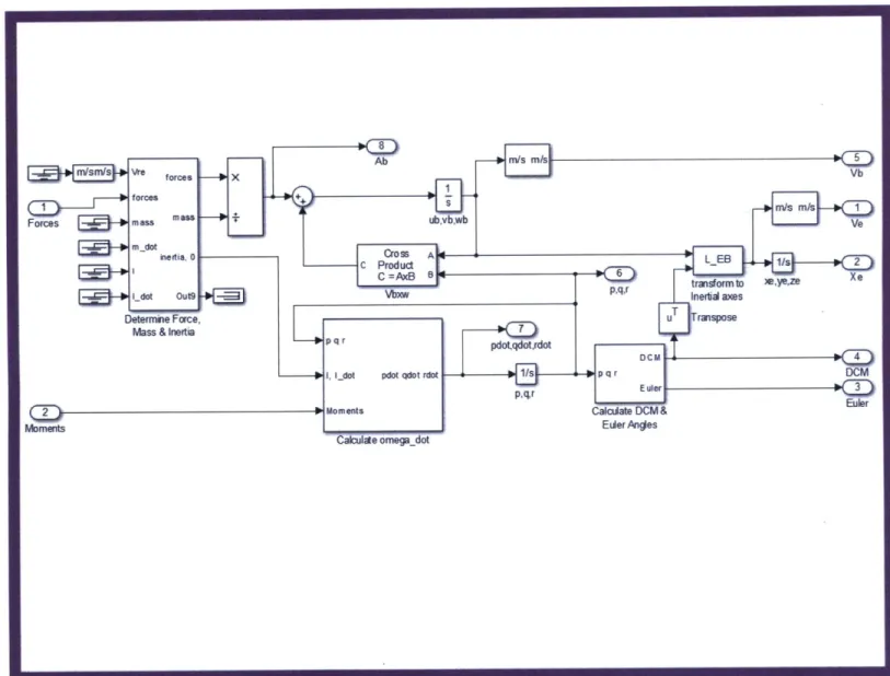
The system dynamics are the quadrotor's response given external forces and moments on the vehicle. This block takes motor commands as inputs. Note that in the sim-ulation, wind speed is also an input so that the system dynamics better match the wind tunnel experimental setup, which will described in Chapter 4. The system dy-namics output actual (or measured) values for the attitude, angular rate, position, and velocity of the quadrotor. Experimentally, this block is the physical vehicle. In simulation, it is an implementation of the equations of motion presented in Chapter

2.

Chapter 2, including both aerodynamic effects and rigid body dynamics. Figure 3-6 shows the implementation of the stock six degree-of-freedom block which propagates the simulated system forward in time given forces and moments on the body as inputs.

3.4

Simulation Results

This section discusses the results obtained from the Simulink implementation of the system described throughout this chapter. The main topics discussed include the steady state attitude response of the vehicle at different operating speeds, forward flight effects on the actuation limits of the vehicle, and the overall performance of the system with the controller presented in Section 3.2.

Values used for the physical parameters and aerodynamic properties of the system for the simulation match the physical parameters and aerodynamic properties of the actual vehicle used in flight experiments to be described in Chapter 6. The methods of obtaining these values are discussed in Chapter 5.

The primary purpose of the simulation is to provide insight into the long term dynamics and limitations of the system described in this chapter. This insight is used to inform the experimental design of the flight tests to be described in Chapter 6. The simulation results will also be compared to experimental results to show the validity of the model presented in Chapter 2.

The simulation starts with zero initial conditions for all states of the quadrotor. The motor thrusts are initialized with forces needed to maintain hover

Fk,o = . (3.20)

4

The simulation commands the following reference inputs

[[Xdes

Ydes Zdes] =

[0.1

m 0 0 (3.21)

[t des Ydes Zdes = [0 0 0] (3.22)

.l'

_ S

HE

[] L~

rL7

'

5 C S Figure 3-5: Simulink Diagram of Block "equations of motion" Corresponds to the System Dynamics Described in Section 3.3 38 J

m

I

Fy-

9

I

_r,

't~ -~

~

%J I- E M--47 060 E E Figure 3-6: Simuliiik Diagram of Block "equations of mnotiorij6DOF (utri'n) 39

and a constant wind speed is added as a direct input into the system dynamics.

3.4.1. Steady State Attitude Response

Unlike at hover conditions, the steady state attitude of a quadrotor in forward flight is nonzero. This is due to the coupling of attitude and velocity that governs quadrotor motion. In this section, the results are generated using a constant wind speed in the negative x direction in the inertial frame. The quadrotor being simulated is equally symmetric about both the x and y body axes. In other words,

Ix = Iy.

Thus, the response of the system would be of the same magnitude and form whether the wind speed was applied along the x or the y inertial axes. Wind speed along the x inertial axis corresponds to a response in pitch while wind speed along the y inertial axis corresponds to roll.

Figure 3-7 shows the steady state value for the quadrotor pitch at wind speeds ranging from 0 to 11 m/s (0 to 25 mph). The figure shows a nonlinear relationship between the steady state pitch and wind speed, a quadratic relationship to be specific

Oss OUcm,re. (3.24)

Similarly,

Oss OC VCm,re. (3.25)

3.4.2

Actuation Limits

Determining the limits of a system is important for informing experimental design for testing the physical quadrotor. Similar operating limits between the simulated and physical system would be evidence to suggest that the model is valid. As in Section 3.4.1, results are generated using a wind in the negative x direction in the inertial

Steady State Attitude 35 30-)2 -a) U A_ 20-CU 0 U 2 4 6 8 10 12 speed (m/s)

Figure 3-7: Steady State Pitch of the Simulated System as a Function of Wind Speed

frame due to the symmetry of the quadrotor.

For the simulated system, the fastest wind speed in which the quadrotor could return to the commanded position within a reasonable time is 13.5 m/s (30 imiph). The quadrotor could make progress towards the commanded position at 14 in/s (31 mph) but displayed an prohibitively long return time (>100 seconds). Figure 3-8 shows the simulated states of the system while in a 14.5 rm/s (32 mph) wind along with the calculated induced thrust forces (T1, T2, T3, T4). Note that the position

in the x direction of tile inertial frame drifts and never turns to return back to the commanded position. The motor thrusts hit their upper limits at 13 seconds and saturate for the rest of the simulation.

Figure 3-9 shows the simulated system response at the maximum controllable speed, 13.5 mn/s (30 mph). Similar to Figure 3-8, the induce thrust forces hit their upper limits, this time around 16 seconds in. However, the position in the x direction of the inertial frame is able to return to the reference position and tihe induced thrust drops below the upper saturation point. Note that the steady state pitch command

Quadrotor States

Velocity in Ineitial Axes

1 - -- - -- - - - -- - - - -- - - -- Velocity in I neftial Axes:1

-- -- --Velocity in Inertial Axes:2 2 -- - q - - - ---- Velocity in Inertial Axes:3

0 5 10 15 20 25 30 35 40 45 50

Position in Inertial Axes

5-- - -* - -- ---- Position in Inertial Axes:1

Position in InertialAxes:2 10- - PositioninI nertialAxes:3 -1 5- -- - - - -- - - - ---20 0 5 10 15 20 25 30 35 40 45 50 EuLei Angles

-20 Eulei Angles:1_{Euler Angles:2}

-40 - - - EulesAngls:3

0 5 10 15 20 25 30 35 40 45 50

Induced Thrust Forces

2-2

2____ T3

0 5 10 15 20 25 30 35 40 45 50

Time (secs)

Figure 3-8: System Response of Simulated Quadrotor Above Maximum Operating

Speed (32 mph). From Top to Bottom, The Plots Show Velocity in the Inertial

Frame, Position in the Inertial Frame, Attitude in Euler Angles, and the Induced

Thrust Forces All With Respect To Time.

at maximum speed is roughly 450.

3.4.3

Control Performance

Response time of the system is largely governed by the controller parameters. The

control gains were chosen to promote stability and controllability over low rise times.

This section discusses the step response of the system when a wind force is

instan-taneously applied to it. The ability of the quadrotor to track reference commands is

also discussed.

In the simulation, a wind force is applied to a quadrotor initialized at hover

instantaneously at t = 0. The quadrotor then attempts to return to a constant

4

Quadrotor States

Velocity in Ilnetial Axes

0 _

-1 - Velocity in InertialAxes:1

.2 - - -Velocity in InertialoAxes:2

- Velocity in Inertial Axes:3

3 5 10 15 20 25 30 35 40 45 50

05

Positon in nneitiel A

2. - - - --Position in Inertial Axes:

-Position in Inetial Axes:2

-6 - - - - - - --I I I 0 5 10 15 20 25 30 35 40 45 50 EuleriAngles 20 1 1 1 1 0 -20 Eder Angles 1 -20 - - - -- --- - -EW ar Angles: 2 Euler Angle3 0 5 10 15 20 25 30 35 40 45 50

Induced Thrust Forces ... ... * 'I ...-..-....--...I...

0 tO1 15 20 25 30 35 40 45 50

Tirro 100s051

Figure 3-9: System Response of Simulated

Quadrotor

at Maximum Operatinig Speed (30 mph) From Top to Bottom, The Plots Show Velocity in the Inertial Frame, Position in the Imertial Frame, Attitude in Euler Angles, anid the Induced Thrust Forces All With Respect To Time.

reference position. To quantify the response time of the system, the rise time (ir) is defined as the earliest time at which the quadrotor is within .01 mi of the reference position. The settling time (t8) is defined as the earliest time at which the quadrotor

is within .005 m of the reference position and remains within t.005 m from the reference position. Table 3.1 provides the values of tr and t8 at speeds from 0 in/s to

13.5 in/s (0 to 30 mph).

The entry in Table 3.1 for a wind speed of 13.5 in/s corresponds to the graphs in Figure 3-9. Note that it has a significantly shorter rise time and later settling time than the next slower speed. This is due to the overshoot (seen in Figure 3-9) in the x position at this wind speed. Slower wind speeds do not result in a similar overshoot

Table 3.1: Rise and Settling Time of the Simulated System at High Speed Wind Speed (m/s) Rise Time, t, (s) Settling Time, t, (s)

0 1 2 2.2 12 17 4.8 20 25 6.7 24 30 9 29 33 11.2 31 35 13.5 23 47

and rather smoothly approach the reference position. Figure 3-10 is a graph of rt and r, as a function of wind speed, up to 11.2 m/s (25 mph). This shows a nonlinear relationship between rise time/settling time and wind speed. Specifically

r ocm,re

2

(3.26) (3.27)

~r

(A LUcm,rel.

To test the ability of the system to track non-constant reference inputs, a sine wave of amplitude 0.5 m and frequency 1 rad/s

X*,,ef =Xref + 0. 5sin t (3.28)

was added to the initial reference x position. Figure 3-11 shows the the system re-sponse while tracking x,*,f with a wind speed of 9 m/s (20 mph). After the expected rise time (Table 3.1), the quadrotor accurately tracks the sine wave. This demon-strates that the quadrotor maintains an adequate amount of control authority while counteracting a wind speed of 9 m/s (20 mph). Similar results are observed up to 12 m/s (27 mph). At higher speeds, the upper limit of the induced thrust forces prevent accurate reference tracking in one direction.

System response time rise time (tr) settling time (t.) 2 4 6 wind speed (m/s) 8 10 12

Figure 3-10: System Response Time as a Function of Wind Speed Quadrotor States

Velocity in Inertial Axes

- V e l c i y in I n e iti a l A e s : 1 Velocy in ner"ialAxes:3

q Velocity in Inertial Ases:3

0 5 10 15 20 25 30 35 40 45 50

Position in Inertial Axes

1 - -III

05 - ____Position in retelAe:

q Position in InestelAxes:2

0

Position in netial Axes:3

4 5 ... 0 5 10 15 20 25 30 35 40 45 50 EderAngles EulenAngess -10 - --20 -30-450 10 15 20 25 Eiule Angles:2 Eule Angles:3

Figure 3-11: Tracking Reference Sine Wave in X-Position at 9 m/s (20 mph)

35 -30 -25 -E 20 15-10 5 0 C 0.5 - -. .. -. 0 -0.5.. . 3540 45 50

3.5

Summary

In this chapter, a full system architecture was described. This system uses successive loop closure to control system dynamics matching those described in Chapter 2. An implementation of the system was built and used to analyze the long term dynamics and limitations of the system. This information will be used to inform the experi-mental design of actual flight tests to be discussed in the following chapters of this thesis.

Chapter 4

Flight Space

This chapter describes the flight testing space created for sustained high speed flight with full state feedback. Flight testing is performed at the Wright Brothers Wind Tunnel at the Massachusetts Institute of Technology [16j. The flight space is equipped with six Vicon motion capture cameras [171 to track the aircraft in real-time, providing pose and velocity information. A picture of the flight space is shown in Figure 4-1 An operation manual for future use of the space can be found in Appendix A.

4.1

Wind Thnnel

The flight space is located in the Wright Brothers Wind Tunnel at the Massachusetts Institute of Technology. This tunnel is a closed return, closed test section wind tunnel with a 7 foot tall by 10 foot wide elliptical cross section and is 15 feet long. A 2,000 HP AC motor powers the Wright Brothers Wind Tunnel. This motor is capable of running at two constant speeds. and the pitch setting of the fan controls the operating airflow speed. Due to a noise constraint, the tunnel is usually run at the lower speed (up to 90 mph), and only occasionally in second speed (up to 150 mph). This is much faster than any flight tests performed for this work and the more relevant limit is the lowest speed attainable, which is about 10 mph. A diagram of the wind tunnel with relevant information is found in Figure 4-2.

TEST SECTION WALIS pW. p00*10

OWNER FACILITY NAME DATE BUILT 0OUNTRY NO Omuneions X.Y,Za 0 soId acauslk SPEED, MACH

_ _ _

~ad#a

_ _o

H. .T. D 1938 UdA a 114se sve chart

STAGNATION REYMOiS Nb RUN DURATION CICUIT POWER SUPPLY

, Raum onge

Piaws Tenaprak" POWER Type Ifan,

to 2 amos oO1f or lasa -2. 5 x 106 valiltad single ratura tan

E(KIPNEINT TYPE OF TEST SCHEME OF THE CIRCUIT, PERFOrOAANCE DIAGRAM

HP*airupplyP ae 4.8.1.6,0.A .07 _____

HpaIrEu4ppITImamftOw 3.60,100,00 pat Gruad x

MID Qf a to 4pol vacuum zasora

Latral 6la Iti Iu

Wallbaana l kite x gsKmI

Ground aGoedtpe-(boo. sucton.

bwinv)-acouaslc batmenf

--DATA ACOUISITION QOMPUTER

Atometle - 48 channele Ultra lei

PLANNED IMPROVEMENTS

Figure 4-2: Wright Brothers Wind Tunnel Diagram [2]

The wind tunnel is made of several key elements, the wind tunnel shell, the propul-sion system, and a set of sensors. The set of sensors installed in the wind tunnel

mea-sure forces and moments on a body installed in the test section. This is the primary use of a wind tunnel, but it is not its purpose for the tests described in this thesis.

Instead of using the wind tunnel to determine aerodynamic properties of an air-craft, it is being used as a proxy for sustained high speed flight. A quadrotor is flown in the wind tunnel to simulate forward flight. To free fly, a different set of sensors are needed both to control the vehicle and to obtain measurements of how the vehicle performs at this flight regime.

4.2

Camera Placement

To allow for full-state feedback and motion tracking to be used for both control and system identification of an aircraft in sustained forward flight, a Vicon motion capture system was integrated into the existing test space within the Wright Brothers Wind Tunnel. A Vicon motion capture system provides real-time pose and velocity information at a rate of 200 Hz. It records groupings of small reflective dots that are rigidly attached to the vehicle being tracked. Images from several cameras are then compared to estimate position, orientation, velocity, and angular rate of the vehicle in 3D space to millimeter precision.

The motion capture system setup in this flight space is comprised of six Vicon motion capture cameras. Four cameras are mounted directly to the exterior of the testing chamber of the wind tunnel. The other two are mounted on tripods as far upstream as possible within the test section. While the tripod mounted cameras are in the freestream, they have no noticeable effect on flight performance as they are far enough upstream that any turbulence they create sufficiently dissipates before reaching the flyable area within the test section. Figure 4-3 is a diagram of the camera placement within the wind tunnel and provides measurements of the flyable area within the test section.

The number and placement of these cameras was heavily constrained by physical limitations in viable mounting locations. Vicon motion capture systems are setup such that the cameras are placed as high up as possible and look down into the space