HAL Id: hal-03041670
https://hal.archives-ouvertes.fr/hal-03041670
Submitted on 3 Feb 2021
HAL is a multi-disciplinary open access archive for the deposit and dissemination of sci-entific research documents, whether they are pub-lished or not. The documents may come from teaching and research institutions in France or abroad, or from public or private research centers.
L’archive ouverte pluridisciplinaire HAL, est destinée au dépôt et à la diffusion de documents scientifiques de niveau recherche, publiés ou non, émanant des établissements d’enseignement et de recherche français ou étrangers, des laboratoires publics ou privés.
Copyright
Complex Canard Explosion in a Fractional-Order
FitzHugh–Nagumo Model
Mohammed-Salah Abdelouahab, René Lozi, Guanrong Chen
To cite this version:
Mohammed-Salah Abdelouahab, René Lozi, Guanrong Chen. Complex Canard Explosion in a Fractional-Order FitzHugh–Nagumo Model. International journal of bifurcation and chaos in applied sciences and engineering , World Scientific Publishing, 2019, 29 (08), pp.1950111. �10.1142/S0218127419501116�. �hal-03041670�
1 Published in: International Journal of Bifurcation and Chaos, Vol. 29, No. 8, ( 2019), pp. 1950111 (22 pages). DOI: 10.1142/S0218127419501116
Personal file
Complex Canard Explosion in a Fractional-Order
FitzHugh–Nagumo Model
Mohammed-Salah Abdelouahab
Laboratory of Mathematics and Their Interactions, University Center of Mila, Algeria
René Lozi
Laboratoire de Mathématiques J.A. Dieudonné, Université Côte d’Azur, Parc Valrose,
06108 Nice Cedex 02, France [email protected]
Guanrong Chen
Department of Electrical Engineering, City University of Hong Kong, Kowloon,
Hong Kong SAR, P. R. China [email protected]
This article investigates the complex phenomena of canard explosion with mixed-mode oscillations, observed from a fractional-order FitzHugh–Nagumo (FFHN) model. To rigorously analyze the dynamics of the FFHN model, a new mathematical notion, referred to as Hopf-like bifurcation (HLB), is introduced. HLB provides a precise definition for the change between a fixed point and an S-asymptotically T-periodic solution of the fractional-order dynamical system, as well as the stability of the FFHN model and the appearance of the HLB. The existence of canard oscillations in the neighborhoods of such HLB points are numerically investigated. Using a new algorithm, referred to as the global-local canard explosion search algorithm, the appearance of various patterns of solutions is revealed, with an increasing number of small amplitude oscillations when two key parameters of the FFHN model are varied. The numbers of such oscillations versus the two parameters, respectively, are perfectly fitted using exponential functions. Finally, it is conjectured that chaos could occur in a two-dimensional fractional-order autonomous dynamical system, with the fractional order close to one. After all, the article demonstrates that the FFHN model is a very simple two-dimensional model with an incredible ability to present the complex dynamics of neurons.
Keywords: FitzHugh–Nagumo model; canard explosion; fractional-order system; mixed-mode
2
1. Introduction
The FitzHugh–Nagumo (FHN) system [FitzHugh, 1961], modeled by a two-dimensional nonlinear differential equation, is one of the most important simplified Hodgkin–Huxley (HH) model of electric circuits, which reproduces fairly the action potential of many types of neurons [Hodgkin & Huxley, 1952]. On one hand, the four-dimensional nonlinear differential equation of the HH model is difficult to study thoroughly either analytically or even numerically; on the other hand, however, due to the innermost properties of two-dimensional dynamical systems highlighted by the Poincaré–Bendixon theorem [Perko, 2002], the FHN model is unable to reproduce many complex dynamics of the corresponding four-dimensional system, such as chaos and hyperchaos. Moreover, mixed-mode oscillations (MMO), which are very common in electroencephalography (EEG) data, can only be modeled by autonomous systems of ordinary differential equations (ODE) with integer dimensions greater than two. Nevertheless, it is possible to find a resolution to this concerned issue between too simple and too complex systems, using fractional derivatives. In fact, there are some recent studies on the fractional-order FitzHugh–Nagumo (FFHN) model [Liu & Xie, 2010; Brandibur & Kaslik, 2018], or its modified versions.
This article further investigates the MMO and the complex canard explosion in the FFHN model. Specifically, the appearance of patterns, from the solution of the FFHN model with a fractional order close to one, is studied as one system parameter is varied, where the number of small-amplitude oscillations increases. Such a phenomenon is impossible to appear from a system with the order of derivative being equal to one, due to the Poincaré–Bendixon theorem. Moreover, to rigorously analyze the FFHN model, it turns out that the classical notion of Hopf bifurcation is not well applicable to fractional-order systems, which cannot have exactly periodic solutions on a finite time interval [Tavazoei & Haeri, 2009]. To deal with this problem, in this article a Hopf-like bifurcation (HLB) theory is introduced, which provides a precise definition for the change between a fixed point and an S-asymptotically T-periodic solution of a fractional-order system. The following study of the complex canard explosion and MMO in the FFHN model leads to a conjecture that chaotic phenomenon can occur in two-dimensional autonomous fractional-order dynamical system with a fractional order close to one. It thus reveals that the FFHN model is a very simple two-dimensional model with an incredible ability to present the complex dynamics of neurons.
Next, in Sec. 2, the definition and properties of canard and MMO will be reviewed. In Sec. 3, some classical results on fractional calculus will be summarized. In Sec. 4, fractional calculus will be further discussed within the context of dynamical systems. The relationship between classical and fractional systems will then be discussed in terms of semigroups. In Sec. 5, the new definition of HLB will be introduced, followed by an analysis of the stability and HLB of the solutions of the FFHN model. In Sec. 6, complex canard explosion and MMO in the FFHN model will be investigated. Finally, in Sec. 7, a brief conclusion will be drawn.
3
2. Canard and Mixed-Mode Oscillations
Solutions of differential equations are trajectories (curves) in the phase space. Many electric and electronic devices, like oscilloscopes, provide also curves as results of sampled physical or physiological phenomena. In biomedical studies, the shapes of these curves are often used to characterize diseases like epilepsy and stroke. Therefore, the study of particular patterns in such trajectory curves is very important in practice.
2.1. Canard and false-canard trajectories
Canard cycles were first discovered and investigated in 1981 by a team of French mathematicians in their pioneering work [Benoît et al., 1981], who coined the French name of
canard for such unexpected complex dynamical behavior.
The conventional canard phenomena highlight the very fast transition (called canard explosion) with respect to a varying parameter, from a large amplitude limit cycle (relaxation) [Fig. 1(a)] to a small-amplitude one [Fig. 1(c)], in a slow–fast ODE, which is also referred to as singularly perturbed systems.
At the beginning of their discovery, this French team used nonstandard analysis as the main mathematical method to analyze canards [Diener, 1984]. Today, the name canard has been widely accepted by the mathematical community and applied to various analyses [Desroches & Jeffrey, 2011]. Its prototypical model is the van der Pol system with constant forcing 𝑎 > 0 [van der Pol, 1926], described in the Liénard plane (x, y) as
{𝑥̇ = 𝑦 −
1 3𝑥
3+ 𝑥,
𝑦̇ = 𝜀(𝑎 − 𝑥). (1)
For a small positive parameter 𝜀 ≪ 1, the variable x is driven by the fast vector field evolving on the fast time scale 𝑡 = 𝜏/𝜀, and y evolves on a slow time scale 𝜏 directed by the slow vector field. Thus, x and y are referred to, respectively, as fast and slow variables. The slow nullcline S, where 𝑥̇ = 0, is called the slow curve or critical manifold.
In the van der Pol system (1), the slow curve is cubic shaped consisting of three branches, the middle one is repelling and connected with two attracting outer branches via two fold-points, as shown in Fig. 1.
Starting from any initial point in the Liénard plane, the solution of (1) is quickly attracted by the fast vector field in a neighborhood of one of the stable parts of the critical manifold. As an example, if the initial point belongs to the upper right-hand side of the Liénard plane, it will follow this stable slow curve downward, directed by the slow vector field, until it reaches the lower fold-point from which it jumps to the other stable part of the critical manifold, as shown in Fig. 1(a). The slow vector field will then drive the solution trajectory upward until it reaches the other fold-point. Then, the trajectory will jump back to the previous stable part of the slow curve, forming a periodic cycle. However, it is possible that, depending on the value of the parameter a, instead of jumping immediately from the first fold-point to the other stable slow curve, the trajectory will follow the unstable part for a while, as shown in Figs. 1(b) and 1(c).
4
Fig. 1. Canard explosion of the van der Pol oscillator for ε = 0.01 happens in an exponentially small parameter interval near a = a* ≈ 0.998740451245, where the transition from relaxation oscillations for (a) a ≤ 0.998740451244, to small-amplitude limit cycles for (c) a ≥ 0.998740451246, happens via (b) canard cycles.
5
This “amplitude bifurcation”, in which the periodic nature of the solution is unchanged, is referred to as canard, because its shape resembles that of a duck [Fig. 1(b), in which both legs are intentionally added].
In general, canard solutions occur in singularly perturbed systems of the form
{𝜀 𝑑𝑥(𝜏) 𝑑𝜏 = 𝑓(𝑥(𝜏), 𝑦(𝜏), 𝜀) , 𝑑𝑦(𝜏) 𝑑𝜏 = 𝑔(𝑥(𝜏), 𝑦(𝜏), 𝜀) , (2)
Where 𝑥 ∈ ℝ𝑛 and 𝑦 ∈ ℝ𝑚 are fast and slow variables, respectively, f and g are sufficiently smooth functions, and 𝜏 denotes the independent variable of (2), called the slow time scale. After a time rescaling to the fast time scale 𝑡 = 𝜏/𝜀 (for 𝜀 ≠ 0), one gets an equivalent system of the form { 𝑑𝑥(𝜏) 𝑑𝜏 = 𝑓(𝑥(𝜏), 𝑦(𝜏), 𝜀) , 𝑑𝑦(𝜏) 𝑑𝜏 = 𝜀𝑔(𝑥(𝜏), 𝑦(𝜏), 𝜀) , (3)
Now, simply write
{𝑥̇ = 𝑓(𝑥, 𝑦, 𝜀),
𝑦̇ = 𝜀𝑔(𝑥, 𝑦, 𝜀), (4) where the dot denotes differentiation with respect to t.
In the limiting case, →0, both systems (2) and (4) read {0 = 𝑓(𝑥, 𝑦, 0),
𝑦̇ = 𝑔(𝑥, 𝑦, 0), (5)
which is a differential-algebraic equation, called the reduced (or slow) subsystem, and {𝑥̇ = 𝑓(𝑥, 𝑦, 0),
𝑦̇ = 0, (6)
called the layer (or fast) subsystem, respectively.
The reduced and the layer subsystems are not equivalent, but they both play a key role in the geometric singular perturbation theory that deals with the dynamical analysis of the full system for 𝜀 > 0 [Wechselberger, 2012]. The critical (slow) manifold 𝑆 = {(𝑥, 𝑦) ∈
ℝ𝑛× ℝ𝑚: 𝑓(𝑥, 𝑦, 0) = 0} for system (2) corresponds to the phase space of the reduced subsystem (5) and the set of equilibria of the layer subsystem (6).
Normal hyperbolicity fails at points on S where the Jacobian 𝐷𝑥𝑓 has (at least) one eigenvalue with zero real part (the most common case where normal hyperbolicity fails is on critical folded manifolds). The subset 𝑆𝑎 ⊂ 𝑆 for which all eigenvalues of 𝐷𝑥𝑓 have negative real parts is called the attracting slow invariant manifold and, similarly, the subset 𝑆𝑟 ⊂ 𝑆 for which all eigenvalues of 𝐷𝑥𝑓 have positive real parts is called the repelling slow invariant
6
Depending upon the directions of the trajectories on the slow manifold, one can define canard trajectories as well as false-canard as follows.
Definition 2.1 (Canard Trajectory) [Shchepakina et al., 2014]. A trajectory of (2) or (4), first
moving along 𝑆𝑎 and then continuing for a while along 𝑆𝑟, is called a canard (or duck) trajectory.
Definition 2.2 (False-Canard Trajectory) [Shchepakina et al., 2014]. A trajectory of (2) or (4),
first moving along 𝑆𝑟 and then continuing for a while along 𝑆𝑎, is called a false-canard trajectory.
2.2. Mixed-mode oscillations
The canard phenomenon is important for better understanding and analyzing of the slow–fast dynamics. For example, the coupling of local passage near a folded singularity, around which canard solutions emerge, with the global return mechanism via relaxation spikes that reset the local dynamics, can explain complex oscillatory patterns called mixed-mode oscillations (MMO). The MMO consists of L large-amplitude (relaxation) oscillations followed by s small-amplitude (subthreshold) oscillations, simply denoted by Ls [Rubin & Wechselberger, 2007]. The topic of MMO is of great importance in various applications, such as cellular electrical and secretory activities [Harvey et al., 2011; Krupa et al., 2008], chemical reactions [Milik & Szmolyan, 2001], optical oscillations [Marino et al., 2011], etc.
In 1952, Alan Lloyd Hodgkin and Andrew Huxley built a mathematical model of electric circuits, which reproduces fairly accurately the action potential of many types of neurons, represented by a nonlinear system of four ordinary differential equations. They were awarded the Nobel Prize for Medicine in 1963 for their works. The complexity of the mathematical analysis of such a four-dimensional nonlinear system had motivated the introduction of various simplifications of the original Hodgkin–Huxley model, the best known (and simplest) one being probably the FitzHugh–Nagumo model proposed in 1961 [FitzHugh, 1961], described by a two-dimensional differential system with cubic nonlinearity. Unfortunately, as indicated by the Poincaré–Bendixon theorem [Perko, 2002], bounded solutions of a two-dimensional autonomous system are attracted to fixed points or period cycles, and they cannot reproduce all the complex dynamics of a four-dimensional dynamical system, such as chaos and hyperchaos. Indeed, MMO dynamics can only be modeled by autonomous systems of ordinary differential equations of greater than two dimensions. The occurrence of such chaotic behavior in the Hodgkin–Huxley model was reported in [Guckenheimer & Oliva, 2002] as well as the occurrence of the MMO in [Rubin & Wechselberger, 2007].
3. Fractional Calculus
Due to the complexity of the dynamical phenomena encountered in nature, more flexibility in the mathematical modeling of such phenomena is needed. To do so, other than increasing the dimension of the dynamical systems, it is possible to resort to fractional-order dynamical systems.
7
The idea of fractional calculus goes back to the early development of the regular calculus [Leibniz, 1962], as a generalization of integration and differentiation to noninteger-orders. It has been found that many systems in interdisciplinary fields can be described by fractional-order differential equations, such as viscoelastic systems, dielectric polarization, and quantum evolution of complex systems [Bagley & Calico, 1991; Sun et al., 1984; Kusnezov et al., 1999].
3.1. Definitions
There are several definitions of fractional derivatives [Podlubny, 1999; Caputo, 1967]. A common one is the Riemann–Liouville definition of fractional derivatives [Podlubny, 1999], given by 𝐷 𝛼 𝑅 𝑡𝛼𝑥(𝑡) = 1 𝛤(𝑚 − 𝛼) 𝑑𝑚 𝑑𝑡𝑚∫ (𝑡 − 𝜏)𝑚−𝛼−1 𝑡 𝑎 𝑥(𝜏)𝑑𝜏 = 𝑑 𝑚 𝑑𝑡𝑚( 𝑗𝑎 𝑡 𝑚−𝛼𝑥(𝑡)), 𝑡 > 𝑎, 𝑚 − 1 ≤ 𝛼 < 𝑚,
where 𝛤 is the gamma function and 𝑗𝑎 𝑡𝛽is the Riemann–Liouville integral operator defined a𝑎 𝑡𝑗𝛽𝑥(𝑡) = 1
𝛤(𝛽)∫ (𝑡 − 𝜏) 𝛽−1 𝑡
𝑎 𝑥(𝜏)𝑑𝜏.
The Laplace transform of the -order Riemann–Liouville differential operator is 𝐿{ 𝐷𝑅0
𝑡𝛼𝑥(𝑡)} = 𝑠𝛼𝐿{𝑥(𝑡)} − ∑𝑚−1𝑘=0 𝑠𝑘[ 𝐷𝑅0 𝑡𝛼−1−𝑘𝑥(𝑡)]𝑡=0. For zero initial condition, one has
𝐿{ 𝐷𝑅0 𝑡𝛼𝑥(𝑡)} = 𝑠𝛼𝐿{𝑥(𝑡)}.
A numerical method often used to compute the Riemann–Liouville fractional derivative is based on the Grünwald–Letnikov definition, given by
𝐷 𝑎 𝐺 𝑡𝛼𝑥(𝑡) = 𝑙𝑖𝑚ℎ→0 1 ℎ𝛼∑ (−1) 𝑘× 𝛤(𝛼+1) 𝑘!𝛤(𝛼−𝑘+1)𝑥(𝑡 − 𝑘ℎ) 𝑘=𝑡−𝛼ℎ 𝑘=0 , (7)
where 𝑡 > 𝑎 and 𝛼 is a positive real number. Its integral form is 𝐷 𝑎 𝐺 𝑡−𝛼𝑥(𝑡) = 𝑙𝑖𝑚 ℎ→0ℎ 𝛼∑ 𝛤(𝛼+𝑘) 𝑘!𝛤(𝛼)𝑥(𝑡 − 𝑘ℎ). 𝑘=𝑡−𝛼 ℎ 𝑘=0 (8)
When f is of class Cm, where m−1 ≤ α < m, both Riemann–Liouville and Grünwald–Letnikov definitions are equivalent [Podlubny, 1999]. Another definition is the Caputo definition of fractional derivatives [Caputo, 1967], given by
𝐷 𝛼𝐶 𝑡𝛼𝑥(𝑡) = 1 𝛤(𝑛 − 𝛼)∫ (𝑡 − 𝜏) 𝑛−𝛼−1 𝑡 𝑎 𝑥(𝑛)(𝜏)𝑑𝜏 = 𝑗𝑛−𝛼(𝑑 𝑛 𝑑𝑡𝑛𝑥(𝑡)) , 𝑡 > 𝑎,
8
where 𝑛 = ⌈𝛼⌉ is the value of 𝛼 rounded up to the nearest integer.
Regarding Lyapunov exponents for fractional chaotic systems, Matlab codes are available in [Danca & Kuznetsov, 2018].
3.2. Basic properties
Next, recall some basic properties of fractional calculus.
Lemma 1 [Diethelm, 2010]. Let 𝛼 > 0, 𝛼 ∉ ℕ and 𝑚 = ⌈𝛼⌉. Moreover, assume that 𝑥 ∈ 𝐶𝑚[𝑎, 𝑏]. Then, 𝐷𝑎𝐶
𝑡𝛼𝑥 ∈ 𝐶𝑚[𝑎, 𝑏] and 𝐷𝑎𝐶 𝑡𝛼𝑥(𝑎) = 0.
Lemma 2 [Diethelm, 2010]. Let 𝑥 ∈ 𝐶𝑘[𝑎, 𝑏] for some 𝑎 < 𝑏 and some 𝑘 ∈ ℕ. Moreover, let 𝛼, 𝛽 > 0, be such that there exists some 𝑙 ∈ ℕ with 𝑙 ≤ 𝑘 and 𝛼, 𝛼 + 𝛽 ∈ [𝑙 − 1, 𝑙]. Then,
𝐷 𝛼𝐶 𝑡 𝛽 𝐷 𝛼 𝐶 𝑡𝛼𝑥(𝑡) = 𝐷𝛼𝐶 𝑡 𝛼+𝛽 𝑥(𝑡) The Laplace transform of the -order Caputo differential operator is
𝐿{ 𝐷0𝑐 𝑡𝛼𝑥(𝑡)} = 𝑠𝛼𝐿{𝑥(𝑡)} − ∑ 𝑠𝛼−1−𝑘𝑥(𝑘)(0) 𝑚−1
𝑘=0
For zero initial conditions, one has
𝐿{ 𝐷0𝑐 𝑡𝛼𝑥(𝑡)} = 𝑠𝛼𝐿{𝑥(𝑡)}
and in this case the above three definitions of the fractional derivative are equivalent.
Remark 3.1. When 𝛼 is close to 𝑚 = ⌈𝛼⌉, the derivatives generated by the above three definitions are close.
4. Classical and Fractional Dynamical Systems
Fractional differential equations are used to describe systems with long-range interactions or systems with power-law memory. Some examples of fractional-order systems in modeling and control are described in [Caponetto et al., 2010].
Now, consider fractional calculus within the scope of dynamical systems. First, recall the definition of a classical (integer-order) dynamical system in terms of semi-group. Then, considering fractional dynamical systems, with the concepts of S-asymptotically and T-periodic solutions, the relationship between both kinds of systems will be discussed in terms of semi-group.
4.1. Classical dynamical systems
A dynamical system in terms of semi-group (in classical definition) on an open set 𝑈 ⊂ ℝ𝑛 is a triplet (T, U,
t) describing the motion of points 𝑥 ∈ 𝑈 with respect to time t in a set of numbers9
T (usually, T = R or T = Z). In addition, 𝜙𝑡(𝑥) = 𝜙(𝑡, 𝑥): T × U → U is a one-parameter family of class-C1 maps satisfying the following properties [Perko, 2002; Kuznetsov, 1995]:
(i) 𝜙0(𝑥) = 𝑥 for all 𝑥 ∈ 𝑈.
(ii) 𝜙𝑡+𝑠(𝑥) = 𝜙𝑡(𝑥) ∘ 𝜙𝑠(𝑥) for all 𝑥 ∈ 𝑈.
This one-parameter family of maps, 𝜙𝑡, is called the flow of the underlying dynamical system.
Remark 4.1 [Perko, 2002]
(1) If T = R, then the triplet (T, U,
t) defines a continuous dynamical system, whereas itdefines a discrete dynamical system if T = Z.
(2) If (R, U,
t) is a continuous dynamical system, then the function𝑓(𝑥) = 𝑑
𝑑𝑡𝜙(𝑡, 𝑥)|𝑡=0 (9)
defines a C1-vector field on U and, for each 𝑥0∈ 𝑈, 𝜙(𝑡, 𝑥0) is the solution of the initial value problem
{𝑥̇ = 𝑓(𝑥),
𝑥(0) = 𝑥0. (10)
(3) Reciprocally, for a given C1-function 𝑓 ∈ 𝐶1(𝑈) and 𝑈 an open subset of ℝ𝑛, the solution
𝜙𝑡(𝑥) of the initial value problem (10), defined for all 𝑡 ∈ ℝ, has the following properties: (i) 𝜙0(𝑥) = 𝑥 for all 𝑥 ∈ 𝑈.
(ii) 𝜙𝑡+𝑠(𝑥) = 𝜙𝑡∘ 𝜙𝑠(𝑥) for all 𝑥 ∈ 𝑈.
Thus, the triplet (R, U,
t) is a dynamical system.4.2. Fractional dynamical systems
Fractional derivative is quite different from the standard integer-order one because it is not local; as a consequence, the solution of a fractional-order equation at time t depends on its memory from the starting time t0 to t [Yazdani & Salarieh, 2011]. In fact, fractional differential
equations are integro-differential equations. Their numerical solution requires large computer memory and long runs of numerical simulations in general.
Consider the following fractional-order initial value problem in terms of Caputo derivative: {𝐶0𝐷𝑡𝛼𝑥(𝑡) = 𝑓(𝑥) ,
𝑥(0) = 𝑥0 , (11)
where 𝑥(𝑡) = (𝑥1(𝑡), ⋯ , 𝑥𝑛(𝑡))𝑇 ∈ 𝑈 ⊂ ℝ𝑛, 𝑓(𝑥) = (𝑓1(𝑥), ⋯ , 𝑓𝑛(𝑥))𝑇, 𝑡 ∈ ℝ+ and 𝛼 ∈ (0,1). This initial value problem can be converted to the following nonlinear Volterra integral equation of the second kind [Kilbas et al., 2006]:
10 𝑥(𝑡) = 𝑥0+ 1 𝛤(𝛼)∫ (𝑡 − 𝜏) 𝛼−1 𝑡 0 𝑓(𝑥(𝜏))𝑑𝜏 (12)
4.2.1. Flows of fractional dynamical systems
Theorem 1 [Diethelm, 2010]. If the function 𝑓: 𝑈 ⊂ ℝ𝑛→ ℝ𝑛 is continuous and satisfies the Lipschitz condition on 𝑈, then for each 𝑥0∈ 𝑈 the initial value problem (11) has an unique maximal continuous solution 𝑥(𝑡).
Based on this theorem, a two-parameter family of mappings can be defined: 𝜙𝑡𝛼(∙) ∶ T × U → U, associated with 𝑥0 ∈ 𝑈, for which there is a unique solution passing through it at 𝑡 = 0.
Thus, for all 𝑥0∈ 𝑈 and taking into account (12), one gets
𝜙𝑡𝛼(𝑥 0) = 𝑥0+ 1 𝛤(𝛼)∫ (𝑡 − 𝜏) 𝛼−1 𝑡 0 𝑓(𝜙𝜏 𝛼(𝑥 0))𝑑𝜏 (13)
Proposition 1. Under the assumptions of Theorem 1, the two-parameter family of mappings 𝜙0𝛼(∙) satisfies the following properties:
(i) 𝜙0𝛼= 𝐼𝑑, and 𝜙𝑡1= 𝜙𝑡. (ii) 𝜙𝑡𝛼∘ 𝜙𝑠𝛼 = 𝜙𝑡+𝑠𝛼 + 𝛥𝑠,𝑡𝛼 (𝑥0), where 𝛥𝑠,𝑡𝛼 (𝑥 0) = 1 𝛤(𝛼)∫ [(𝑠 − 𝜏) 𝛼−1− (𝑡 + 𝑠 − 𝜏)𝛼−1]𝑓(𝜙 𝜏𝛼 𝑠 0 (𝑥0))𝑑𝜏, for all 𝑠, 𝑡 ∈ ℝ +. Proof. The statement (i) is obvious. It can be verified by substituting 𝑡 = 0 and 𝛼 = 1
respectively in (13).
For (ii), letting 𝑥0∈ 𝑈 and then using (13), one obtains
𝜙𝑡𝛼∘ 𝜙𝑠𝛼(𝑥 0) = 𝜙𝑠𝛼(𝑥0) + 1 𝛤(𝛼)∫ (𝑡 − 𝜏) 𝛼−1𝑓(𝜙 𝜏𝛼 𝑡 0 (𝜙𝑠𝛼(𝑥 0)))𝑑𝜏 = 𝑥0+ 1 𝛤(𝛼)∫ (𝑠 − 𝜏) 𝛼−1𝑓(𝜙 𝜏𝛼 𝑠 0 (𝑥0))𝑑𝜏 + 1 𝛤(𝛼)∫ (𝑡 − 𝜏) 𝛼−1𝑓(𝜙 𝜏𝛼 𝑡 0 (𝜙𝑠𝛼(𝑥 0)))𝑑𝜏 = 𝑥0+ 1 𝛤(𝛼)∫ (𝑠 − 𝜏) 𝛼−1𝑓(𝜙 𝜏𝛼 𝑠 0 (𝑥0))𝑑𝜏 + 1 𝛤(𝛼)∫ (𝑡 + 𝑠 − 𝜏) 𝛼−1𝑓(𝜙 𝜏−𝑠𝛼 𝑡+𝑠 𝑠 (𝜙𝑠𝛼(𝑥 0)))𝑑𝜏 = 𝑥0+ 1 𝛤(𝛼)∫ (𝑠 − 𝜏) 𝛼−1𝑓(𝜑 𝜏𝛼 𝑠 0 (𝑥0))𝑑𝜏 − 1 𝛤(𝛼)∫ (𝑡 + 𝑠 − 𝜏) 𝛼−1𝑓(𝜑 𝜏𝛼 𝑠 0 (𝑥0))𝑑𝜏 + 1 𝛤(𝛼)∫ (𝑡 + 𝑠 − 𝜏) 𝛼−1𝑓(𝜑 𝜏𝛼 𝑡+𝑠 0 (𝑥0))𝑑𝜏 (14)
11 where {𝜑𝜏 𝛼(𝑥 0) = 𝜙𝜏𝛼(𝑥0), 0 ≤ 𝜏 ≤ 𝑠 𝜑𝜏𝛼(𝑥0) = 𝜙𝜏−𝑠𝛼 (𝜙𝑠𝛼(𝑥0)), 𝜏 > 𝑠. It can be easily verified that, 𝜑𝜏𝛼(𝑥
0) is continuous with respect to 𝜏. Thus,
𝜑𝑡+𝑠𝛼 (𝑥0) = 𝑥0+ 1 𝛤(𝛼)∫ (𝑡 + 𝑠 − 𝜏) 𝛼−1× 𝑓(𝜑 𝜏𝛼 𝑡+𝑠 0 (𝑥0))𝑑𝜏 and 𝜑𝜏+𝑠𝛼 (𝑥0) is a solution of (11). By the uniqueness of the solution, one has
𝜑𝑡+𝑠𝛼 (𝑥0) = 𝜙𝑡+𝑠𝛼 (𝑥0). Substituting it into (14) yields
𝜙𝑡𝛼∘ 𝜙𝑠𝛼= 𝜙𝑡+𝑠𝛼 + 𝛥𝑠,𝑡𝛼 (𝑥0)
Clearly, if 𝛼 = 1 then 𝛥𝑠,𝑡𝛼 (𝑥0) = 0 for all 𝑠, 𝑡 ∈ ℝ+; however, for 0 < 𝛼 < 1 then 𝛥𝑠,𝑡𝛼 (𝑥0) = 0 for all f only if 𝑡 = 0 or 𝑠 = 0. Thus, for 0 < 𝛼 < 1, the triplet (ℝ+, 𝑈, 𝜙𝑡𝛼) is not a dynamical system in terms of semi-group.
Definition 4.1. Let 0 < 𝛼 < 1. Then, under the above assumptions, the triplet (ℝ+, 𝑈, 𝜙𝑡𝛼) is called a fractional dynamical system.
Figure 2 illustrates the discrepancy between solutions of a fractional dynamical system and solutions of a classical dynamical system.
12
Since the semi-group property is not satisfied by the flow of a fractional dynamical system, a trajectory in the phase space of such a system can intersect itself (without giving a periodic orbit) after a certain time t. This will never happen in the integer-order setting.
4.2.2. Generalized fractional-order dynamical systems in semi-group
Now, it is to show that a generalized fractional order dynamical system can be converted to a classical dynamical system (in terms of semi-group) of a greater dimension.
Lemma 3. If the function f is of class 𝐶1(𝑈), then there exists a 𝐶(ℝ
+× 𝑈). function 𝑔𝑓𝛼 , such that the fractional-order initial value problem (11) is equivalent to the integer-order nonautonomous initial value problem:
{𝑥̇(𝑡) = 𝑔𝑓
𝛼(𝑡, 𝑥)
𝑥(0) = 𝑥0
(15)
Proof. Applying the fractional operator 𝐶0𝐷𝑡1−𝛼 to both sides of the first equation in (11), and taking into account Lemma 2, yields
𝑥̇(𝑡) = 𝐷𝐶0
𝑡1−𝛼𝑓(𝑥) (16)
Putting 𝑔𝑓𝛼= 𝐷0𝐶 𝑡1−𝛼𝑓(𝑥) since 𝑓 ∈ 𝐶1(𝑈), by Lemma 1 one obtains 𝑔𝑓𝛼 ∈ 𝐶(ℝ+× 𝑈). Thus, the fractional-order initial value problem (11) is equivalent to the integer-order nonautonomous initial value problem (15), where 𝑔𝑓𝛼(𝑡, 𝑥) = 𝐷0𝐶 𝑡1−𝛼𝑓(𝑥).
Theorem 2. If the function f and its fractional derivative 𝐶0𝐷𝑡1−𝛼𝑓(𝑥) are of class 𝐶1, then the fractional-order initial value problem (11) defines an (n+1)-dimensional dynamical system,
(ℝ+, 𝑈, 𝜙𝑡𝛼) in terms of semi-group, where 𝑈 ⊂ ℝ𝑛+1.
Proof. By Lemma 3, the fractional-order initial value problem (11) is equivalent to the integer
order nonautonomous initial value problem (15), which can be converted to an (n + 1)-dimensional autonomous system by denoting 𝑥𝑛+1= 𝑡, which yields 𝑥̇𝑛+1= 1. The resultant initial value problem reads
{𝑥̇(𝑡) = 𝐹(𝑥, 𝛼),
𝑥(0) = 𝑥0. (17)
where 𝐹𝑖(𝑥, 𝛼) = 𝐷𝐶0 𝑥𝑛+1 1−𝛼𝑓
𝑖(𝑥), for 𝑖 = 1, ⋯ , 𝑛, and 𝐹𝑛+1(𝑥, 𝛼) = 1. Thus, 𝐹 is a 𝐶1-function. Consequently, by Remark 4.1, the initial value problem (17) defines an (n + 1)-dimensional dynamical system, (ℝ+, 𝑈, 𝜙𝑡𝛼).
4.2.3. S-asymptotically T-periodic solutions
The nonexistence of periodic solutions in fractional order autonomous systems with bounded lower terminal was proved in [Tavazoei & Haeri, 2009; Tavazoei et al., 2009] and the existence of periodic solutions in fractional-order autonomous systems with unbounded lower terminal or with fixed memory lengths was discussed in [Yazdani & Salarieh, 2011; Kang et al., 2015; Abdelouahab & Hamri, 2016].
13
Now, recall the definitions of asymptotically T-periodic and S-asymptotically T-periodic functions [Henriquez et al., 2008], which can occur as solutions of a fractional-order autonomous system with fixed bounded lower terminal, instead of a normal T-periodic solution [Yazdani & Salarieh, 2011; Kang et al., 2015].
Let 𝐶𝑏(ℝ+, ℝ𝑛) denote the space of continuous and bounded functions 𝑥: ℝ+→ ℝ𝑛 , equipped with the norm ‖∙‖∞
Definition 4.2. A function 𝑥 ∈ 𝐶𝑏(ℝ+, ℝ𝑛) is called asymptotically T-periodic, if there exists a bounded continuous T-periodic function u and a bounded continuous function v with
𝑙𝑖𝑚𝑡→∞𝑣 (𝑡) = 0 such that 𝑥 = 𝑢 + 𝑣. The collection of all these functions is denoted by
𝐴𝑃𝑇(ℝ+, ℝ𝑛).
Definition 4.3. A function 𝑥 ∈ 𝐶𝑏(ℝ+, ℝ𝑛) is called S-asymptotically T-periodic, if there exists T > 0 such that 𝑙𝑖𝑚𝑡→∞(𝑥(𝑡 + 𝑇) − 𝑥(𝑡)) = 0. In this case, T is said to be an asymptotic period of x. The collection of all these functions is denoted by 𝑆𝐴𝑃𝑇(ℝ+, ℝ𝑛).
The sets 𝐴𝑃𝑇(ℝ+, ℝ𝑛) and 𝑆𝐴𝑃𝑇(ℝ+, ℝ𝑛), equipped with the norm ‖∙‖∞, are Banach spaces.
Moreover,
𝐴𝑃𝑇(ℝ+, ℝ𝑛) ⊂ 𝑆𝐴𝑃𝑇(ℝ+, ℝ𝑛).
The existence of S-asymptotically T-periodic solutions in a class of fractional-order differential equations and fractional-order functional integro-differential equations have been studied in [Cuevas & Cesar de Souza, 2010].
5. Hopf-Like Bifurcation in the Fractional-Order FitzHugh–
Nagumo Model
This section studies the FFHN model, for which a mathematical notion of Hopf-like bifurcation (HLB) is introduced and analyzed.
5.1. FitzHugh–Nagumo model
As mentioned in the Introduction, as an approximation of the Hodgkin–Huxley model [Hodgkin & Huxley, 1952], the FitzHugh–Nagumo model [FitzHugh, 1961] has become popular. An electrical circuit equivalent to this model was constructed by Nagumo et al. [1962], as shown in Fig. 3.
This electrical model consists of a voltage variable v (membrane potential) with cubic nonlinearity that allows regenerative self-excitation via a positive feedback, and a recovery variable w, which describes the combined effect of ion channels, with a linear term that affords a slower negative feedback.
14 { 𝑑𝑣 𝑑𝑡 = 𝑣 − 1 3𝑣 3 − 𝑤 + 𝐼, 𝑑𝑤 𝑑𝑡 = 1 𝑇(𝑣 + 𝑎 − 𝑏𝑤), (18)
with parameters I, a, b and T. With a change of variables, x = v, y = w, and 𝜀 = 1/𝑇, the system becomes {𝑥̇ = 𝑥 − 1 3𝑥 3− 𝑦 + 𝐼, 𝑦̇ = 𝜀(𝑥 + 𝑎 − 𝑏𝑦). (19)
Fig. 3. Electrical circuit of the FitzHugh–Nagumo model.
One can see that, if b = I = 0 and 𝑥 → −𝑥, Eq. (19) is exactly the van der Pol system (1).
5.2. Fractional-order FitzHugh–Nagumo model
In 1983, Jonscher [1983] demonstrated that the ideal capacitor having integer-order constitutive equation
𝑣(𝑡) =1
𝐶𝑞(𝑡) ⇔ 𝐼(𝑡) = 𝐶 𝑑𝑣(𝑡)
𝑑𝑡 ,
cannot exist in nature, where I(t) is the current through the capacitor, v(t) is the voltage across the capacitor, and C is the capacitance of the capacitor.
In 1991, Westerlund [1991] demonstrated that the inductor is fractional in nature and its better constitutive relation is
𝑣(𝑡) = 𝐿𝐷𝛼𝐼(𝑡), where the constant 𝛼 is related to the proximity effect.
15
In 1994 [Westerlund & Ekstam, 1994] proposed that also a more realistic capacitor could be represented with a fractional-order constitutive equation, as
𝐼(𝑡) = 𝐶𝐷𝛼𝑣(𝑡),
where the constant 𝛼 (derivative order) is related to the loss of the capacitor.
Based on the above observations, it is natural to introduce the fractional-order version of the FitzHugh–Nagumo model [Liu & Xie, 2010], using the fractional-order constitutive equations of capacitor and inductor. In so doing, system (19) can be transformed to its fractional version {𝐷 𝛼1𝑥 = 𝑥 −1 3𝑥 3− 𝑦 + 𝐼, 𝐷𝛼2𝑦 = 𝜀(𝑥 + 𝑎 − 𝑏𝑦), (20)
where 𝛼1 and 𝛼2 are constants related to the loss of the capacitor and the proximity effect of the inductor, respectively.
5.3. Stability and Hopf-like bifurcation
As a first approach to analyzing the FFHN model, only the case of 𝛼1= 𝛼2= 𝛼 ∈ (0,2) is analyzed in this section.
5.3.1. Fixed points and stability
In order to have a unique fixed point of the FFHN model, some parameter restrictions are first introduced.
The existence of this fixed point is characterized by the following proposition.
Proposition 2. For all 𝑎, 𝑏, 𝐼 ∈ ℝ satisfying
−4 (1 −1 𝑏) 3 + 9 (𝐼 −𝑎 𝑏) 2 > 0,
the system (20) has a unique equilibrium point
𝐸 = (𝑥𝑒(𝑏), 𝑦𝑒(𝑏)) where 𝑥𝑒(𝑏) = √−𝑞 + √−𝛥27 2 3 + √−𝑞 − √ −𝛥 27 2 , 3 𝑦𝑒(𝑏) = 𝑥𝑒(𝑏) −1 3𝑥𝑒 3(𝑏) + 𝐼, 𝛥 = −(4𝑝3+ 27𝑞2) , 𝑝 = −3 (1 −1 𝑏) , and 𝑞 = −3 (𝐼 − 𝑎 𝑏) , Proof. A fixed point 𝐸 = (𝑥𝑒, 𝑦𝑒) of system (20) is a solution of
16 {𝑥 − 1 3𝑥 3− 𝑦 + 𝐼 = 0, 𝜀(𝑥 + 𝑎 − 𝑏𝑦) = 0. (21) Thus, {𝑦 = 𝑥 − 1 3𝑥 3+ 𝐼, 𝑥 + 𝑎 − 𝑏 (𝑥 −1 3𝑥 3+ 𝐼) = 0. (22)
Since the second equation is cubic, its canonical form reads
𝑥3+ 𝑝𝑥 + 𝑞 = 0, (23) where 𝑝 = −3 (1 −1 𝑏), 𝑞 = −3 (𝐼 − 𝑎 𝑏) . Assume that −4 (1 −1 𝑏) 3 + 9 (𝐼 −𝑎 𝑏) 2 > 0. Then, −(4𝑝3+ 27𝑞2) = 𝛥 < 0 .
Using Cardan’s cubic method, Eq. (23) has a unique real solution
𝑥𝑒(𝑏) = √−𝑞 + √−𝛥27 2 3 + √−𝑞 − √ −𝛥 27 2 , 3
For the stability analysis, the following theorem will be applied.
Theorem 3 [Matignon, 1996; Moze & Sabatier, 2005]. The following fractional-order linear autonomous system: {𝐷 𝛼𝑋 = 𝐴𝑋, 𝑋(0) = 𝑋0 𝑋 ∈ ℝ 𝑛 0 < 𝛼 < 2 𝑎𝑛𝑑 𝐴 ∈ ℝ𝑛× ℝ𝑛,
is locally asymptotically stable if and only if
𝑚𝑖𝑛
𝑖 |𝑎𝑟𝑔( 𝜆𝑖)| > 𝛼 𝜋
2, 𝑖 = 1,2, ⋯ , 𝑛.
The following proposition for fractional-order nonlinear systems will also be utilized.
Proposition 3 [Abdelouahab et al., 2010]. Let E be an equilibrium point of the fractional-order nonlinear system
17 𝐷𝛼 = 𝑓(𝑥) 0 < 𝛼 < 2.
If the eigenvalues of the Jacobian matrix 𝐴 =𝜕𝑓
𝜕𝑥|𝐸 satisfy
𝑚𝑖𝑛
𝑖 |𝑎𝑟𝑔( 𝜆𝑖)| > 𝛼 𝜋
2, 𝑖 = 1,2, ⋯ , 𝑛. then the system is asymptotically stable at the equilibrium point 𝐸.
The Jacobian matrix of system (20) at the equilibrium point 𝐸 is
𝐽𝐸= (1 − 𝑥𝑒
2(𝑏) −1
𝜀 −𝑏𝜀),
and the characteristic polynomial reads
𝑃(𝜆) = 𝜆2+ (𝑥𝑒2(𝑏) + 𝑏𝜀 − 1)𝜆 + 𝜀(1 + 𝑏(𝑥𝑒2(𝑏) − 1)).
For (𝑥𝑒2(𝑏) − 𝑏𝜀 − 1)2< 4𝜀, the Jacobian matrix 𝐽𝐸 has a pair of complex conjugate eigenvalues:
𝜆± =
−(𝑥𝑒2(𝑏)+𝑏𝜀−1)±𝑖√−(𝑥𝑒2(𝑏)−𝑏𝜀−1)2+4𝜀
2 .
According to Proposition 3, the fixed point 𝐸 of (20) is locally asymptotically stable if
|𝑎𝑟𝑐𝑡𝑎𝑛 (√−(𝑥𝑒 2(𝑏) − 𝑏𝜀 − 1)2+ 4𝜀 𝑥𝑒2(𝑏) + 𝑏𝜀 − 1 )| >𝛼 2. 5.3.2. Hopf-like bifurcation
Since exact periodic solutions are not expected in fractional-order autonomous systems [Tavazoei & Haeri, 2009; Yazdani & Salarieh, 2011; Tavazoei et al., 2009; Kang et al., 2015], the classical notion of Hopf bifurcation does not exist in such systems. Thus, it is natural to introduce a new notion that will be meaningful for this kind of systems.
Here, the idea is to define Hopf-like bifurcation (HLB) in fractional-order systems as a local bifurcation, where a fixed point of the underlying dynamical system changes its stability property as a pair of complex conjugate eigenvalues 𝜆∓ of the Jacobian matrix at the fixed point cross the boundary of an angular sector |𝑎𝑟𝑔( 𝜆∓)| = 𝛼𝜋
2 of the complex plane, giving rise (or vanishing) to a small-amplitude S-asymptotically T-periodic solution. In fact, some criteria of HLB in fractional-order systems were already introduced in [Abdelouahab et al., 2012], although it was not called “Hopf-like” therein.
To analyze HLB in system (20) at its unique fixed point 𝐸 = (𝑥𝑒(𝑏), 𝑦𝑒(𝑏)) with respect to the parameter b and the parameter 𝛼, respectively, a function 𝑀(𝑏, 𝛼) is defined as follows:
𝑀(𝑏, 𝛼) = 𝛼𝜋
2− |𝑎𝑟𝑐𝑡𝑎𝑛 (
√−(𝑥𝑒2(𝑏) − 𝑏𝜀 − 1)2+ 4𝜀
𝑥𝑒2(𝑏) + 𝑏𝜀 − 1
18
Then, some conditions on the parameters to generate HLB are derived.
Proposition 4 (HLB with Respect to the Parameter b). Let the fractional order 𝛼 be fixed and b* be the value of solution b to 𝑀(𝑏, 𝛼) = 0. If
(𝑥𝑒2(𝑏) − 𝑏𝜀 − 1)2 < 4𝜀 and (2𝑥𝑒(𝑏) 𝑑𝑥𝑒(𝑏) 𝑑𝑏 (𝑏 2𝜀 − 𝑏(𝑥 𝑒2(𝑏) − 1) − 2) + (𝑥𝑒2(𝑏) − 1)2− 𝑏𝜀(𝑥𝑒2(𝑏) − 1) − 2𝜀)| 𝑏=𝑏∗ ≠ 0
then system (20) undergoes an HLB at the unique equilibrium point 𝐸, when 𝑏 = 𝑏 ∗.
Proof. For (𝑥𝑒2(𝑏) − 𝑏𝜀 − 1)2 < 4𝜀 the Jacobian matrix 𝐽𝐸 has a pair of complex conjugate eigenvalues:
𝜆± =
−(𝑥𝑒2(𝑏)+𝑏𝜀−1)±𝑖√−(𝑥𝑒2(𝑏)−𝑏𝜀−1)2+4𝜀
2 .
Let 𝑏 ∗ be the value of solution 𝑏 to 𝑀(𝑏, 𝛼) = 0, and denote
𝑢(𝑏) =√−(𝑥𝑒
2(𝑏) − 𝑏𝜀 − 1)2+ 4𝜀
𝑥𝑒2(𝑏) + 𝑏𝜀 − 1 Then, one has
𝑀(𝑏, 𝛼) = 𝛼𝜋 2− |𝑎𝑟𝑐𝑡𝑎𝑛( 𝑢(𝑏))|, so that 𝜕𝑀(𝑏, 𝛼) 𝜕𝑏 = ± 𝑑(𝑢(𝑏) 𝑑𝑏 1 + 𝑢2(𝑏)
It then follows that 𝜕𝑀(𝑏,𝛼)
𝜕𝑏 has the same sign as ± 𝑑𝑢(𝑏)
𝑑𝑏 . Let us suppose that
(2𝑥𝑒(𝑏) 𝑑𝑥𝑒(𝑏) 𝑑𝑏 (𝑏 2𝜀 − 𝑏(𝑥 𝑒2(𝑏) − 1) − 2) + (𝑥𝑒2(𝑏) − 1)2− 𝑏𝜀(𝑥𝑒2(𝑏) − 1) − 2𝜀)| 𝑏=𝑏∗ ≠ 0 Then ±𝑑𝑢(𝑏) 𝑑𝑏 |𝑏=𝑏∗ = ± 𝑑 𝑑𝑏( √−(𝑥𝑒2(𝑏) − 𝑏𝜀 − 1)2+ 4𝜀 𝑥𝑒2(𝑏) + 𝑏𝜀 − 1 )| 𝑏=𝑏∗ = ±2𝜀2𝑥𝑒(𝑏) 𝑑𝑥𝑒(𝑏) 𝑑𝑏 (𝑏2𝜀 − 𝑏(𝑥𝑒2(𝑏) − 1) − 2) + (𝑥𝑒2(𝑏) − 1)2− 𝑏𝜀(𝑥𝑒2(𝑏) − 1) − 2𝜀 (𝑥𝑒2(𝑏) − 𝑏𝜀 − 1)2√4𝜀 − (𝑥𝑒2(𝑏) − 𝑏𝜀 − 1)2 | 𝑏=𝑏∗
19
Fig. 4. (a) HLB curve in the (𝑏, 𝛼) parameter space and (b) curve of the derivative 𝜕𝑀(𝑏,𝛼)
𝜕𝑏 |𝑏=𝑏∗ versus the bifurcation value b*.
Thus, according to the HLB criteria introduced in [Abdelouahab et al., 2012], system (20) undergoes a Hopf-like bifurcation at 𝐸, when b=b*.
The parameter values are chosen as 𝑎 = 0.75, 𝐼 = 0.41, 𝜀 = 0.05, and the two other parameters 0 < 𝑏 < 𝑏̄ and 𝛼 ∈ (0,2) are considered as control parameters, where 𝑏̄ ≈ 1.4371898.
Figure 4(a) shows the critical curve 𝛾 of the following equation:
𝑀(𝑏, 𝛼) = 𝛼𝜋
2− 𝑚𝑖𝑛𝑖 |𝑎𝑟𝑔(𝜆𝑖(𝑏))| = 0,
which separates stable and unstable regions in the (𝑏, 𝛼) parameter space. Figure 4(b) shows the curve of the derivative function 𝜕𝑀(𝑏,𝛼)
𝜕𝑏 |𝑏=𝑏∗ versus the bifurcation value b*, which is strictly negative.
All conditions for HLB [Abdelouahab et al., 2012] are satisfied at each point in the curve
𝛾, implying that when parameters move from stable to unstable regions in the (𝑏, 𝛼) parameter space, the fixed point 𝐸 loses its stability near the critical curve 𝛾. This gives rise to
small-20
amplitude oscillatory behavior and allows the possibility of developing fractional-order canard solutions.
5.3.3. Canard cycles
To investigate the canard phenomenon in the FFHN model, the theory of singularly perturbed system will be applied.
In the limiting case as 𝜀 → 0, the reduced fractional-order equation of system (20), which characterizes the slow dynamics, reads
{𝑥 − 1 3𝑥
2− 𝑦 + 𝐼 = 0 ,
𝐷𝛼𝑦 = 𝑥 + −𝑏𝑦 , (25)
and the fractional-order layer equation, which characterizes the fast dynamics, reads
{𝐷
𝛼= 𝑥 −1 3𝑥
3+ 𝐼 − 𝑦 = 𝑓(𝑥) − 𝑦 ,
𝐷𝛼𝑦 = 0 , (26)
The critical manifold is given by
𝑆0 = {(𝑥, 𝑦) ∈ ℝ2|𝑦 = 𝑥 −1 3𝑥
3+ 𝐼 − 𝑦 = 𝑓(𝑥)}
Thus, 𝑓′(𝑥) = 1 − 𝑥2, so 𝑆0 has two folds, (𝑥, 𝑦) = (±1, ± 2
3+ 𝐼) which separates the two attractive branches 𝑆𝑎, where 𝑓′(𝑥) < 0, from the repulsive branch 𝑆𝑟, where 𝑓′(𝑥) > 0, as shown in Fig. 5.
Fig. 5. Fractional-order fast and slow subsystems of system (20). Single arrows indicate slow motions along the slow curve 𝑆0. Double arrows indicate fast motions outside 𝑆0, which has two attracting branches, 𝑆𝑎, and one repelling branch, 𝑆𝑟, separated by fold-points (dots) of the slow curve, corresponding to saddle-node bifurcation points of the fast subsystem.
21
6. Numerical Analysis of Complex Canard Explosion and
Mixed-Mode Oscillations
Proceeding as in the integer-order setting, by examining the existence of canard oscillations in the neighborhood of the HLB points (b*, α*) versus the two parameters b and α, respectively, system (20) is numerically integrated over the interval [0, tf ]. In doing so, the Grünwald–
Letnikov approximation method is applied, where the integrating step size is h = 0.01, with the initial conditions x0 = xe(b) and y0 = ye(b)−0.005. In order to accelerate the calculation
processes, the short memory length principle [Podlubny, 1999; Abdelouahab & Hamri, 2016] is adopted, with memory length L = 100.
6.1. Complex canard explosion and mixed-mode oscillations versus parameter b
To illustrate the complex canard explosion versus the parameter b, fix α = 0.95 and consider
b as the bifurcation parameter in interval (0, 1.2). Then, HLB occurs at b* ≈ 0.83, while oscillations can be observed for b < 0.83.
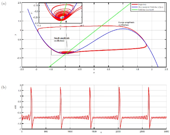
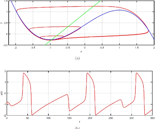
Fig. 6. Mixed-mode oscillations observed in the two-dimensional fractional-order system (20), with b = 0.815: (a) phase portrait and (b) time evolution of x.
22
Figure 6 displays the phase portrait and the time evolution of system (20) at b = 0.815. From this figure, a new phenomenon can be observed that cannot be observed from the integer-order setting. There is an alternation between oscillations of distinct large- and small-amplitude “mixed-mode oscillations”. This phenomenon cannot occur in smooth two-dimensional autonomous integer-order systems, thanks to the semi-group property of the flow 𝜙 (namely, for any 𝑡, 𝑠 ∈ ℝ, 𝑥 ∈ 𝑈 ⊂ ℝ𝑛, one has 𝜙
𝑡(𝜙𝑠𝑥)) = 𝜙𝑡+𝑠(𝑥)). This property does not allow any trajectory to cross itself without giving periodic orbits (due to the Cauchy–Lipschitz theorem). But, this property is not verified in the following fractional-order flow:
𝜙
0 𝑡𝛼( 𝜙0 𝑠𝛼𝑥)) ≠ 𝜙0 𝑡+𝑠𝛼 (𝑥)
because of the memory dependency, as mentioned in Sec. 3. Consequently, a trajectory in the fractional order flow can cross itself without giving rise to any periodic orbit, allowing for the appearance of MMO in smooth two-dimensional autonomous fractional order systems.
For b = 0.7, one can only observe large-amplitude oscillations. For b = 0.83, one can only observe small-amplitude oscillations (with amplitude close to zero). When the parameter b is varied from b = 0.7 to b = 0.83, the number of small-amplitude oscillations, 𝑁𝑆𝐴𝑂(𝑏), which occurs between every two successive large-amplitude oscillations, changes from
𝑁𝑆𝐴𝑂(0.7) = 0 to 𝑁𝑆𝐴𝑂(0.83) = +∞.
To localize infinitesimal subintervals for which 𝑁𝑆𝐴𝑂(𝑏) increases by 1, where canard cycle can be developed, a “Global-Local Canard Explosion Search Algorithm” (GLCESA) is applied, with two search steps as follows:
• Global search step
The parameter b is varied in a global loop by a dynamic step size hd and “Parameter Subinterval Detections” 𝑃𝑆𝐷 = [𝑏𝑖, 𝑏𝑖+ ℎ𝑑] in which an increment of 𝑁𝑆𝐴𝑂 by 1 is determined.
• Local high-precision search step
The parameter b is varied within a local loop, based on a successive division of each subinterval,
𝑃𝑆𝐷 = [𝑏𝑖, 𝑏𝑖−1] (bisection method), to obtain the “Infinitesimal Canard Explosion Parameter Subinterval” 𝐼𝐶𝐸𝑃𝑆 = [𝑎𝑐𝑘, 𝑏𝑐𝑘], with high precision.
First, the subinterval 𝐶𝐸𝑃𝑆 is initialized at 𝑃𝑆𝐷; then, at each step, it is divided into two halves, by computing the midpoint 𝑐𝑘and the value of 𝑁𝑆𝐴𝑂(𝑐𝑘) at that point.
The proposed GLCESA is described in more detail in Appendix A.
Here, the 𝐼𝐶𝐸𝑃𝑆 is estimated with accuracy of 10−13, so the number of iterations of the algorithm in the local search step is NI ≥ E(13 ln(10)+ ln(hd)/ ln(2)) iterations, where 𝐸(⋅) is the integer part.
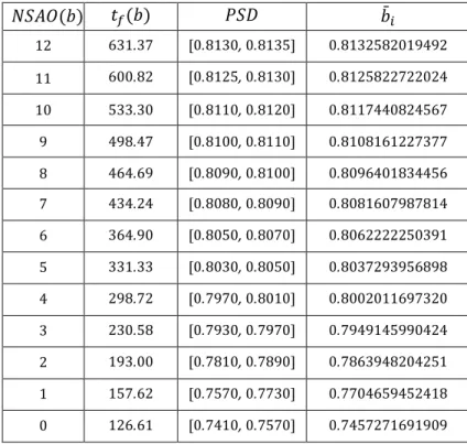
A total of 13 canard explosion parameter subintervals, 𝐶𝑃𝐸𝑆 = [𝑏̄𝑖, 𝑏̄𝑖+ 10−13], 𝑖 =
23
From this table, one can see that the amplitude of the last small oscillation increases, as the parameter b decreases. Then, one can observe canard explosion within an exponentially small neighborhood of b*, where the transition from small-amplitude oscillation (stationary-like behavior) to large-amplitude oscillation (relaxation oscillation) happens a fractional canard solution, as illustrated in Fig. 8, where the canard explosion occurs in the parameter subinterval
𝐼𝐶𝐸𝑃𝑆 = [0.7863948204251, 0.7863948204252]. For b = 0.7863948204252, there are three small-amplitude oscillations between the first and the second large-amplitude oscillations; for
b = 0.7863948204251, there are only two small amplitude oscillations.
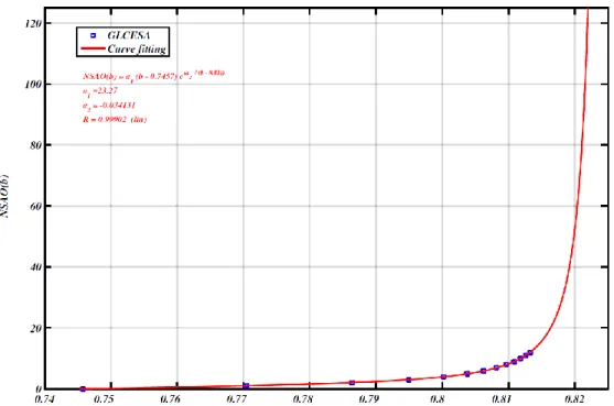
To find the best fitted curve for the points (𝑏̄𝑖, 𝑁𝑆𝐴𝑂(𝑏̄𝑖)), 𝑖 = 1,2, ⋯ ,13, that represents the general trend, the “Esyfit” Matlab tool is used. For this purpose, choose a function that can meet the constraints, namely: 𝑁𝑆𝐴𝑂(0.7) = 0 and 𝑙𝑖𝑚𝛼→0.83𝑁 𝑆𝐴𝑂(𝑏) = +∞. A candidate function is
𝑁𝑆𝐴𝑂(𝑏) = 𝑎1(𝑏 − 0.7)𝑒(𝑎2/(𝑏−0.83))
which yields 𝑎1≈ 23.27, 𝑎2≈ −0.034131, and the correlation coefficient 𝑅 ≈ 0.99902, indicating a good fitting as shown in Fig. 7.
Table 1. Some canard explosion parameter subintervals: 𝐶𝑃𝐸𝑆 = [𝑏̄𝑖, 𝑏̄𝑖+ 10−13], 𝑖 = 1,2, ⋯ ,13, with their corresponding NSAO, tf and PSD, determined by the proposed GLCESA as the parameter b is varied.
𝑁𝑆𝐴𝑂(𝑏) 𝑡𝑓(𝑏) 𝑃𝑆𝐷 𝑏̄𝑖 12 631.37 [0.8130, 0.8135] 0.8132582019492 11 600.82 [0.8125, 0.8130] 0.8125822722024 10 533.30 [0.8110, 0.8120] 0.8117440824567 9 498.47 [0.8100, 0.8110] 0.8108161227377 8 464.69 [0.8090, 0.8100] 0.8096401834456 7 434.24 [0.8080, 0.8090] 0.8081607987814 6 364.90 [0.8050, 0.8070] 0.8062222250391 5 331.33 [0.8030, 0.8050] 0.8037293956898 4 298.72 [0.7970, 0.8010] 0.8002011697320 3 230.58 [0.7930, 0.7970] 0.7949145990424 2 193.00 [0.7810, 0.7890] 0.7863948204251 1 157.62 [0.7570, 0.7730] 0.7704659452418 0 126.61 [0.7410, 0.7570] 0.7457271691909
24
Fig. 7. Curve fitting points (𝑏̄𝑖, 𝑁𝑆𝐴𝑂(𝑏̄𝑖)), generated using the proposed GLCESA. The fitted function is
𝑁𝑆𝐴𝑂(𝑏) = 23.27(𝑏 − 0.7)𝑒(−0.034131/(𝑏−0.83)).
Fig. 8. Canard solutions observed from fractional-order system (20): (a) phase portrait for b = 0.7863948204251, (b) time evolution of x for b = 0.7863948204251, (c) phase portrait for b = 0.7863948204252 and (d) time evolution of x for b =0.7863948204252.
25
Fig. 8. (Continued)
Fig. 9. Curve fitting points (𝑁𝑆𝐴𝑂(𝛼̄𝑖), 𝛼̄𝑖, ) generated using the proposed GLCESA. The fitted function is
26
6.2. Complex canard explosion
To illustrate the complex canard explosion versus fractional order α, fix b = 0.8 and consider α as the bifurcation parameter in the interval (0,1). Then, HLB occurs at α* = 0.9251.
For α = 0.97, one can only observe large amplitude oscillations; for α = 0.9251, one can only observe small-amplitude oscillations (with amplitude close to zero). When the fractional order α is varied, from α = 0.97 to α = 0.9251, the number of small-amplitude oscillations
𝑁𝑆𝐴𝑂(𝛼), which occur between every two successive large amplitude oscillations, change from
𝑁𝑆𝐴𝑂(0.97) = 0 to 𝑁𝑆𝐴𝑂(0.9251) = +∞. To localize the infinitesimal subintervals on which
𝑁𝑆𝐴𝑂 increases by 1, where canard cycles can be developed, we proceed as in the above subsection, for which the proposed GLCESA is applied.
A total of 13 canard explosion parameter subintervals, 𝐶𝑃𝐸𝑆 = [𝛼̄𝑖, 𝛼̄𝑖+ 10−13], 𝑖 =
1,2, ⋯ ,13, are stored in Table 2, with their corresponding 𝑁𝑆𝐴𝑂, tf and 𝑃𝑆𝐷.
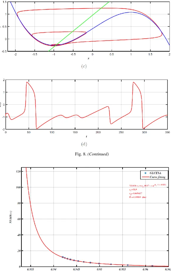
From this table one can see that the amplitude of the last small oscillation increases as the fractional order α increases. Then, one can observe canard explosion within an exponentially small neighborhood of α*, where the transition from small-amplitude oscillation (stationary-like behavior) to large-amplitude oscillation (relaxation oscillation) happens via fractional canard solutions, as illustrated in Fig. 10, where the canard explosion occurs in the parameter subinterval 𝐶𝐸𝑃𝑆 = [0.9677434182069, 0.9677434182070] (for 𝛼 = 0.9677434182069, there is one small-amplitude oscillation between the first and the second large amplitude oscillations; for 𝛼 = 0.9677434182070, there is zero small-amplitude oscillations). To find the best fitted curve for the points (𝛼̄𝑖, 𝑁𝑆𝐴𝑂(𝛼̄𝑖)), 𝑖 = 1,2, ⋯ ,13, that represents their general trend, again the “Esyfit” Matlab tool is applied. To this end, choose a function that can meet the constraints, namely: 𝑁𝑆𝐴𝑂(0.97) = 0 and 𝑙𝑖𝑚𝛼→0.9251𝑁 𝑆𝐴𝑂(𝛼) = +∞. The candidate function is
𝑁𝑆𝐴𝑂(𝛼) = 𝑎1(0.97 − 𝛼)𝑒(𝑎2/(𝛼−0.925)).
Thus, one obtains 𝑎1≈ 38.9, 𝑎2≈ 0.040417 and the correlation coefficient 𝑅 ≈ 0.99908, indicating a good fitting, as shown in Fig. 9.
As previously mentioned, a trajectory of asmooth two-dimensional autonomous fractional order system can cross itself without giving rise to any periodic orbit. This shows that the Poincaré–Bendixson theorem, which guarantees the nonexistence of the chaotic phenomena in smooth two-dimensional autonomous systems, is only valid for the integer-order setting. When fractional-order dynamical systems are considered, there is more flexibility of models with the possibility of having chaotic solutions in dimension two. Moreover, even if the fractional order is close to one, such chaotic phenomenon can still arise. This leads to the following interesting conjecture.
Conjecture 1. Chaos can exist in two-dimensional autonomous fractional-order dynamical systems with the fractional order close to one.
The chaotic phenomena, if existing in a two dimensional autonomous fractional-order dynamical system, are likely to have only one positive Lyapunov exponent (repelling) and one
27
negative Lyapunov exponent (attracting), which is larger than the positive Lyapunov exponent in magnitude, having no zero ones [Danca et al., 2018].
Table 2. Some canard explosion parameter subintervals 𝐶𝑃𝐸𝑆 = [𝛼̄𝑖, 𝛼̄𝑖+ 10−13], 𝑖 = 1,2, ⋯ ,13, with their corresponding 𝑁𝑆𝐴𝑂, tf and
𝑃𝑆𝐷, determined using the proposed GLCESA, as the parameter α is varied. 𝑁𝑆𝐴𝑂(𝛼) 𝑡𝑓(𝛼) 𝑃𝑆𝐷 𝛼̄𝑖 12 610.69 [0.9419, 0.9422] 0.9419865649848 11 577.39 [0.9422, 0.9425] 0.9424658807848 10 539.24 [0.9428, 0.9434] 0.9430130879415 9 504.79 [0.9434, 0.9440] 0.9436601053460 8 472.07 [0.9440, 0.9446] 0.9444332599613 7 403.39 [0.9452, 0.9462] 0.9453719917284 6 366.80 [0.9462, 0.9472] 0.9465298907124 5 333.88 [0.9472, 0.9482] 0.9479883536832 4 296.46 [0.9492, 0.9512] 0.9498957361566 3 233.18 [0.9512, 0.9532] 0.9524863819805 2 189.15 [0.9552, 0.9592] 0.9561361504262 1 155.12 [0.9592, 0.9632] 0.9614783464776 0 113.26 [0.9672, 0.9752] 0.9677434182069
7. Conclusions
This article has investigated the complex phenomena of canard explosion with mixed-mode oscillations (MMO), which can be observed from a fractional-order FitzHugh–Nagumo (FFHN) model.
The study has highlighted the appearance of patterns of solutions with increasing number of small-amplitude oscillations in each of such patterns, as one parameter of the FFHN model is varied when fractional order is close to one.
To rigorously analyze such complex dynamics of the FFHN model, a new mathematical tool is introduced, namely the Hopf-like bifurcation (HLB), which gives rise to a precise definition of the change between a fixed point and an S-asymptotically T-periodic solution of the fractional-order system.
The study has also highlighted the relationship between classical and fractional systems in terms of semi-group.
Then, the stability and HLB analyses of the FFHN model have been carefully analyzed, confirming the existence of canard oscillations in the neighborhood of a HLB point versus either the system parameter b, or the fractional order α. A new algorithm, named the Global-Local Canard Explosion Search Algorithm, has been designed and verified. The simulation results
28
show that one can perfectly fit the number of small-amplitude oscillations in each pattern versus the lengths of the intervals for both parameters between two different patterns, using exponential functions.
Fig. 10. Canard solution observed from fractional-order system (20): (a) phase portrait for α = 0.9677434182069, (b) time evolution of x for α = 0.9677434182069, (c) phase portrait for α = 0.9677434182070 and (d) time evolution of x for α = 0.9677434182070.
29
Fig. 10. (Continued)
Finally, it was conjectured that chaos can exist in two-dimensional autonomous fractional order dynamical systems with the fractional order close to one.
In summary, this study reveals that the FFHN model as a very simple two-dimensional fractional order system offers an incredible possibility for describing the complex dynamics of neuron.
References
Abdelouahab, M. S., Hamri, N. E. & Wang, J. W. [2010] “Chaos control of a fractional-order financial system,”
Math. Probl. Eng. 2010, 270646.
Abdelouahab, M. S., Hamri, N. E. & Wang, J. W. [2012] “Hopf bifurcation and chaos in fractional-order modified hybrid optical system,” Nonlin. Dyn. 69, 275–284.
Abdelouahab, M. S. & Hamri, N. E. [2016] “The Grünwald–Letnikov fractional-order derivative with fixed memory length,” Mediterr. J. Math. 13, 557–572.
Bagley, R. L. & Calico, R. A. [1991] “Fractional order state equations for the control of viscoelastically damped structures,” J. Guid. Contr. Dyn. 14, 304–311.
Benoît, E., Callot, J. F., Diener, F. & Diener, M. [1981] “Chasse au canard,” Collect. Math. 31, 37–119.
Brandibur, O. & Kaslik, E. [2018] “Stability of two-component incommensurate fractional-order systems and applications to the investigation of a FitzHugh–Nagumo neuronal model,” Math. Meth. Appl. Sci. 41, 7182–7194.
30
Caponetto, R., Dongola, G., Fortuna, L. & Peträ´s, I. [2010] Fractional Order Systems: Modeling and Control
Applications (World Scientific, Singapore).
Caputo, M. [1967] “Linear models of dissipation whose Q is almost frequency independent-II,” Geophys. J. Roy.
Astron. Soc. 13, 529–539.
Cuevas, C. & Cesar de Souza, J. [2010] “Existence of S-asymptotically ω-periodic solutions for fractional order functional integro-differential equations with infinite delay,” Nonlin. Anal.: Th. Meth. Appl. 72, 1683–1689. Danca, M. F. & Kuznetsov, N. V. [2018] “Matlab code for Lyapunov exponents of fractional-order systems,” Int.
J. Bifurcation and Chaos 28, 1850067-1–14.
Danca, M. F., Fećkan, M., Kuznetsov, N. V. & Chen, G. [2018] “Fractional-order PWC systems without zero Lyapunov exponents,” Nonlin. Dyn. 92, 1061– 1078.
Desroches, M. & Jeffrey, M. R. [2011] “Canards and curvature: The ‘smallness of ’ in slow–fast dynamics,”
Proc. Roy. Soc. A 467, 2404–2421.
Diener, M. [1984] “The canard unchained or how fast/slow dynamical problems bifurcate,” Math. Intell. 6, 38– 49.
Diethelm, K. [2010] The Analysis of Fractional Differential Equations (Springer, Berlin).
FitzHugh, R. [1961] “Impulses and physiological states in theoretical models of nerve membrane,” Biophys. J. 1, 445–466.
Guckenheimer, J. & Oliva, R. [2002] “Chaos in the Hodgkin–Huxley model,” SIAM J. Appl. Dyn. Syst. 1, 105– 114.
Harvey, E., Kirk, V., Wechselberger, M. & Sneyd, J. [2011] “Multiple time scales, mixed mode oscillations and canards in models of intracellular calcium dynamics,” J. Nonlin. Sci. 21, 639–683.
Henriquez, H. R., Pierri, M. & Tàboas, P. [2008] “On S-asymptotically ω-periodic functions on Banach spaces and applications,” J. Math. Anal. Appl. 343, 1119–1130.
Hodgkin, A. L. & Huxley, A. F. [1952] “A quantitative description of membrane current and its application to conduction and excitation in nerve,” J. Physiol. 117, 500–544.
Jonscher, A. K. [1983] Dielectric Relaxation in Solids (Chelsea Dielectric Press, London).
Kang, Y.M., Xie, Y., Lu, J. C. & Jiang, J. [2015] “On the non-existence of non-constant exact periodic solutions in a class of the Caputo fractional-order dynamical systems,” Nonlin. Dyn. 82, 1259–1267.
Kilbas, A. A., Srivastava, H. M. & Trujillo, J. J. [2006] Theory and Applications of Fractional Differential
Equations (Elsevier, NY).
Krupa, M., Popovic, N., Kopell, N. & Rotstein, H. G. [2008] “Mixed-mode oscillations in a three timescale model for the dopaminergic neuron,” Chaos 18, 015106
Kusnezov, D., Bulgac, A. & Dang, G. D. [1999] “Quantum Levy processes and fractional kinetics,” Phys. Rev.
Lett. 82, 1136–1139.
Kuznetsov, Y. A. [1995] Elements of Applied Bifurcation Theory (Springer, Berlin).
Leibniz, G. W. [1962] Leibnizens Mathematische Schriften (Georg Ohms Verlagsbuch Handlung Hildesheim). Liu, Y. & Xie, Y. [2010] “Dynamical characteristics of the fractional-order FitzHugh–Nagumo model neuron and its synchronization,” Acta Phys. Sin. 59, 2147–2155.
Marino, F., Ciszak, M., Abdalah, S. F., Al-Naimee, K., Meucci, R. & Arecchi, F. T. [2011] “Mixed-mode oscillations via canard explosions in light-emitting diodes with optoelectronic feedback,” Phys. Rev. E 84, 047201. Matignon, D. [1996] “Stability results in fractional differential equation with applications to control processing,”
Proc. Multiconf. Comput. Eng. Syst. Appl. (IMICS), IEEE-SMC 2, 963–968.
Milik, A. & Szmolyan, P. [2001] “Multiple time scales and canards in a chemical oscillator,” Multiple-Time- Scale
Dynamical Systems, IMA Vol. Math. Appl., Vol. 122 (Springer, NY), pp. 117–140.
Moze, M. & Sabatier, J. [2005] “LMI tools for stability analysis of fractional systems,” Proc. ASME Int. Design
31
Nagumo, J., Arimoto, S. & Yoshizawa, S. [1962] “An active pulse transmission line simulating nerve axon,” Proc.
IRE 50, 2061–2070.
Perko, L. [2002] Differential Equations and Dynamical Systems (Springer, NY). Podlubny, I. [1999] Fractional Differential Equations (Academic Press, San Diego).
Rubin, J. & Wechselberger, M. [2007] “Giant Squid — Hidden Canard: The 3D geometry of the Hodgkin Huxley model,” Biol. Cybern. 97, 5–32.
Shchepakina, E., Sobolev, V. & Mortell, M. P. [2014] Singular Perturbations: Introduction to System Order
Reduction Methods with Applications, Lecture Notes in Mathematics (Springer).
Sun, H. H., Abdelwahab, A. A. & Onaral, B. [1984] “Linear approximation of transfer function with a pole of fractional order,” IEEE Trans. Autom. Contr. 29, 441–444.
Tavazoei, M. S. & Haeri, M. [2009] “A proof for non-existence of periodic solutions in time invariant fractional order systems,” Automatica 45, 1886– 1890.
Tavazoei, M. S., Haeri, M., Attari, M., Bolouki, S. & Siami, M. [2009] “More details on analysis of fractional-order van der Pol oscillator,” J. Vibr. Contr. 15, 803–819.
van der Pol, B. [1926] “On ‘relaxation oscillations’,” London, Edinburgh, and Dublin Phil. Mag. J. Sci. 7, 978– 992.
Wechselberger, M. [2012] “`A propos de canards (Apropos canards),” Trans. Am. Math. Soc. 364, 3289– 3309. Westerlund, S. [1991] “Dead matter has memory!” Physica Scripta 43, 174.
Westerlund, S. & Ekstam, S. [1994] “Capacitor theory,” IEEE Trans. Dielectr. Electr. Insul. 1, 826–839.
Yazdani, M. & Salarieh, H. [2011] “On the existence of periodic solutions in time-invariant fractional order systems,” Automatica 47, 1834–1837.
Appendix A
Global-Local Canard Explosion Search Algorithm
The Global-Local Canard Explosion Search Algorithm (GLCESA) is summarized as follows:
Inputs:
α; Fractional-order derivative tf ; Final time integration
h; Discretization time step of the system L; Memory length
System parameters a; I; ε;
bi; bf ; Initial and final values of the parameter b
Outputs:
NSAO; Numbers of small-amplitude oscillations PSD; Parameter subintervals detection
CEPS; Canard explosion parameter subintervals
Step 1. Initialization of:
tf ; First length of integration interval of the system hd; Initial value of dynamical step size
32
k = 0; i = 1; Initializing index b(i) = bi; Initializing parameter Step 2. Global-local search
Solve system (20) and calculate NSAO(b(i))
Step 2.1. Global search
while b(i) ≥ bf (Global search loop) do i = i + 1; b(i) = bi + (i − 1) ∗ hd;
Solve the system (20) and calculate NSAO(b(i))
Δ = NSAO(b(i − 1)) − NSAO(b(i))
if Δ = 1 then k = k + 1
PSD(k) = [bi, bi−1]
ack = bi, bck = bi−1
Step 2.2. Local search subalgorithm
while |bck - ack| > 10−13 (local loop of high precision search) do
𝑐𝑘=
𝑎𝑐𝑘+ 𝑏𝑐𝑘
2
Solve system (20) and calculate NSAO(c(k))
if NSAO(c(k)) = NSAO(bc(k)) then bck = ck;
else ack = ck;
end if endwhile
ICEPSk = [ack, bck] else if Δ = 0 ‘the parameter step size hd is relatively small’ then
hd = 2∗ hd
else if Δ > 1 ‘the parameter step size hd is relatively large’ then bi = bi − hd;
hd = hd/Δ i = i − 1; end if end while