• Aucun résultat trouvé

A coherent framework for learning spatiotemporal piecewise-geodesic trajectories from longitudinal manifold-valued data

N/A
N/A
Protected

Academic year: 2021

Partager "A coherent framework for learning spatiotemporal piecewise-geodesic trajectories from longitudinal manifold-valued data"

Copied!
40
0
0

Texte intégral

(1)

HAL Id: hal-01646298

https://hal.archives-ouvertes.fr/hal-01646298v4

Submitted on 10 Apr 2020

HAL is a multi-disciplinary open access

archive for the deposit and dissemination of

sci-entific research documents, whether they are

pub-lished or not. The documents may come from

teaching and research institutions in France or

abroad, or from public or private research centers.

L’archive ouverte pluridisciplinaire HAL, est

destinée au dépôt et à la diffusion de documents

scientifiques de niveau recherche, publiés ou non,

émanant des établissements d’enseignement et de

recherche français ou étrangers, des laboratoires

publics ou privés.

A coherent framework for learning spatiotemporal

piecewise-geodesic trajectories from longitudinal

manifold-valued data

Juliette Chevallier, Vianney Debavelaere, Stéphanie Allassonnière

To cite this version:

Juliette Chevallier, Vianney Debavelaere, Stéphanie Allassonnière. A coherent framework for learning

spatiotemporal piecewise-geodesic trajectories from longitudinal manifold-valued data. SIAM Journal

on Imaging Sciences, Society for Industrial and Applied Mathematics, In press, �10.1137/20M1328026�.

�hal-01646298v4�

(2)

A Coherent Framework for Learning Spatiotemporal

Piecewise-Geodesic Trajectories from Longitudinal

Manifold-Valued Data

I

Juliette Chevalliera,∗, Vianney Debavelaerea, Stéphanie Allassonnièreb aCentre de Mathématiques Appliquées, Écoles polytechniqye, Palaiseau, France bCentre de Recherche des Cordeliers, Université Paris-Descartes, Paris, France

Abstract

This paper provides a coherent framework for studying longitudinal manifold-valued data. We introduce a Bayesian mixed-effects model which allows estimating both a group-representative piecewise-geodesic tra-jectory in the Riemannian space of shape and inter-individual variability. We prove the existence of the maximum a posteriori estimate and its asymptotic consistency under reasonable assumptions. Due to the non-linearity of the proposed model, we use a stochastic version of the Expectation-Maximization algorithm to estimate the model parameters. Our simulations show that our model is not noise-sensitive and succeeds in explaining various paths of progression.

Keywords: Bayesian estimation, EM like algorithm, Longitudinal data, MCMC methods, Nonlinear mixed-effects model, Spatiotemporal analysis

1. Introduction

Beyond transversal studies, temporal evolution of phenomena is a field of growing interest. Indeed, to understand a phenomenon, it appears more suitable to compare the evolution of its markers over time than to do so at a given stage.

Chemotherapy monitoring is based on the follow-up of scores over time to report on the progression of the disease. Actually, rather than tumors aspect or size, oncologists asses that a given treatment is efficient from the moment it results in a decrease of tumor volume. The same applies to neurodegenerative disorders, such as Alzheimer’s disease or Parkinson’s disease: rather than neuronal degeneration itself which is a natural consequence of cerebral aging, the pathological nature of such diseases lies in the rate of progression of this senescence. The study of longitudinal data is not restricted to medical applications and proves successful in various fields of application such as computer vision, automatic detection of facial emotions, social sciences, etc.

Recent advances in medical imaging offer new opportunities for follow-ups. We can now carry out patients’ monitoring free of invasive measures, such as biopsies. Hence, to provide everyone with the best possible treatment, there is a need for prediction methods that allow to grasp quickly the efficiency of a possible treatment based solely on image-type data. Consequently, designing models that deal with medical images and more generally extracted features and shapes from these images is very important for application-related uses. This paper provides a coherent framework for studying such longitudinal structured data.

IThis work was financed by a public grant as part of the Investissement d’avenir, project reference ANR-11 LABX-0056-LMH

and by the Fondation de la recherche médicale, under contract number DBI20131228564.

Corresponding author

Email address: juliette.chevallier@polytechnique.edu (Juliette Chevallier)

(3)

1.1. The Use of Riemannian Geometry for the Study of Longitudinal Data

Anatomical data – and most of structured data – have been successfully modeled as points on a Rieman-nian manifold, i.e. as points on a smooth manifold equipped with a RiemanRieman-nian metric tensor. These spaces are often called shape spaces. The choice of the shape space and its metric tensor is driven by the type of data in the study (Charlier et al.,2017;Charon and Trouvé,2013;Klassen et al.,2004;Trouvé and Younes,

2015;Vaillant and Glaunès, 2005). Geometrical properties of shape manifolds have been properly defined over the last decades. Moreover, according to the Whitney embedding theorem (Gallot et al.,2004), as the shape spaces are second-countable, they are always embedded in a real d-dimensional Euclidean space, the space of measurements, which leads us to consider the shape manifold as a submanifold of this Euclidean space.

Formally, we call shape space the unique orbit of the transitive action of a group G of deformations on a set M ⊂ Rdof shapes. Then all the shapes can be obtained by deformation of a template shape. Most of the

time, G is nothing more than the group C1(Rd) of the C1-diffeomorphisms of Rd. Due to the construction

by group action, we can endow this manifold with a distance that quantifies the cost of deformation from a shape to another (Younes, 2010). More precisely, if we assume that G is endowed with a right-invariant metric dG, then we can endow M with the pseudo-metric defined by

∀ x, y ∈ M, dM(x, y) = inf

g∈G {dG(Id, g) | g · x = y} .

One method (among others like the diffeomorphic demons algorithm (Vercauteren et al.,2009)) which allows such a framework is the large deformation diffeomorphic metric mapping (LDDMM) (Beg et al.,2005;Dupuis et al., 1998) that we will use in this paper. The main idea of LDDMM is to allow for, accordingly to their name, large deformations of space while keeping control over them, particularly through smoothness. To do so, we restrict the group of deformations G to a sub-group GV ⊂ G of well-behaving deformations, in a sense

we are going to specify.

Let V be a set of vector fields over Rn, whose norms correspond to the cost of deformation. We assume

that V can be endowed with a Hilbert space structure and is continuously embedded into the space C1 0(Rn)

of the diffeomorphisms that decay at infinity and whose differentials decay at infinity. Let L2

V = L2([0, 1], V )

the set of all time-dependent vector fields v = (vt)t∈[0,1] which are L2-integrable with respect to t. We then

define the group GV referred to above by setting GV = { φv1| v ∈ L2V }, where φv1 is the flow at time t = 1

associated with the differential equation ∂tφvt = vt◦ φtv, φv0 = Id (Younes, 2010). We want to emphasize

here that the application t 7→ φv

t does not have a priori its values in Rd but rather in the Riemannian

manifold of shapes M. Note that φv

1 ∈ C1(Rn) and that the differential equation above admits a unique

solution for each initial condition (Younes, 2010). Lastly, there exists a vector field v able to transport a configuration of the shape space into another while minimizing the cost of deformation (Younes,2010), i.e. the following minimum is reached for a certain v in L2

V, and the cost of deformation from a shape x to

another shape y is given by

∀ x, y ∈ M, dM(x, y) = inf v∈L2V  Z 1 0 kvtk 2 V dt 1/2 φv1· x = y  .

Therefore, the temporal evolution of empirical data may be modeled as a parametric curve in the space of measurements and more precisely as a noisy version of an underlying curve living on the Riemannian shape submanifold. Given a cohort of individuals followed over a given period, we thus observe discreet samples of such a curve for each subject. We call this set of observations a longitudinal data set. Figure1 illustrates this understanding of the data.

1.2. Models with a Medical Focus for the Study of Longitudinal Data

Reaction-diffusion based tumor growth models have demonstrated their efficiency for cancer monitoring (Konukoglu et al.,2010;Rekik et al.,2013). The idea of these methods is to model the tumor growth with a “simple" PDE model, involving few parameters which are estimated from series of CT-scan or MRI (Colin

(4)

et al., 2010;Saut et al., 2014). For therapy planning purposes, such methods can reinforce the decision to wait without specific treatment, in case of slow progression of the tumor, thus preventing heavy treatment. However, such methods cover images but not shapes or whatever else type of data, e.g. scores. Besides, even for images, as these models rely on reaction-diffusion equations, they can only apply for situations in which the observed phenomenon is linked to diffusion dynamics. As a consequence, these models can apply to untreated cancer but not to treated-one nor to multiple sclerosis monitoring, neurodegenerative disease follow-up, like Alzheimer’s or Parkinson’s diseases, or more complicated framework. Last, they cannot predict the response to a given molecule and so help in the choice of the appropriate one, nor in the choice of an appropriate sequence of molecules.

Mixed-effects models have proved to be effective for the study of longitudinal data sets (Laird and Ware,

1982), especially for medical purposes (Comets et al.,2010;Milliken and Edland,2000;Ribba et al.,2014). Indeed, mixed-effects models provide a general and flexible framework to study complex data which depends on unobserved variables, such as longitudinal data sets. They consist of two parts: fixed effects which describe the data at the population level and random effects that are associated with individual experimental units. In the framework of longitudinal analysis, through mixed-effects models, one can explain in two steps, both a representative path of the evolution of the whole population and individual-specific progressions. Given a longitudinal data set, a representative trajectory and its variability are first estimated. Then, we can define subject-specific trajectories with respect to global progression.

Building on the geodesic regression model (Fletcher,2011), the generative and hierarchical model ( Mu-ralidharan and Fletcher, 2012) allows for the analysis of longitudinal Riemannian manifold-valued data. Each individual is assumed to follow a geodesic trajectory, which is itself a random perturbation of a mean geodesic trajectory. The geodesic hierarchical model for diffeomorphisms (Singh et al.,2013,2014) exploits the close link between groups of deformations and shape spaces and consists in estimating a geodesic tra-jectory of diffeomorphisms at the population scale. However, random effects of both models depend heavily on the first time of observation, and thus a change in this first time involves a corresponding change in the estimated value for these effects. The first time of acquisition does not have insofar any meaningful place in the modeling process and there is thus a need for a model robust to changes in the time origin.

Discriminating spatial deformations, linked with the intrinsic geometry of observed shapes, from temporal deformations, related to acquisition constraints, is a mean of freeing oneself from this limitation. The idea of spatio-temporal atlas (Durrleman et al.,2009,2013) is to estimate a continuous trajectory of shapes such that each observation corresponds to the evaluation at a given time of a spatio-temporal deformation of this template scenario. To our knowledge, this model is the first to break spatial and temporal deformations up. Moreover, it can handle massive and heterogeneous data such as low dimensional anatomic shapes. Several other models are also based on the concept of time warp (Delor et al., 2013; Yang et al., 2011). However, since the temporal parameterization introduced in these models is statistically non-parametric, it is difficult to estimate. In the same vein and based on the notion of time warps, a kind of generalization of the geodesic hierarchical model (Muralidharan and Fletcher,2012) has been proposed byKim et al.(2017): the Riemannian nonlinear mixed-effects model. However, due to the high complexity of the model, it is impossible to estimate the parameters accurately.

Specifically for the study of brain senescence processes,Lorenzi et al.(2015) propose to distinguish natural aging due to anatomical age from pathological aging. However, despite appealing features, this model is not easy to extend to other scope of applications. The temporal alignment in longitudinal data analysis is also an efficient way to geometrically compare trajectories (Su et al.,2014a,b). Here, the authors propose to use the temporal registration to align the different trajectories. Despite good results for comparing trajectories, the interpretation of the temporal parameterization is lost. However, within medical applications, the time parametrization reveals information on the data patient’s state of health and has to be considered.

The recent generic spatio-temporal model (Schiratti et al.,2015,2017) takes into account all the problems raised above. This model was built to grant temporal and spatial inter-subject variability through individual variations of a common time-line and parallel shifting of a representative trajectory. Each individual tra-jectory has its own intrinsic geometric pattern through spatial variability and its own time parametrization through time variability. In terms of modeling, the time variability allows some individuals to follow the same progression path but at a different age and with possibly a different pace. This model was notably

(5)

applied to early detection of Alzheimer’s disease and proved thereat to be efficient (Bilgel et al., 2016). Morevoer, this model was recently improved in order to increase its applicability (Bône et al., 2018;Koval et al.,2017,2018) and is still the subject of intensive research (Debavelaere et al.,2019). However, whether it is the original model or its extensions, they all make a strong hypothesis to build their model as they assume the characteristic evolution to be geodesic, i.e. that the characteristic trajectory is the shortest path between the initial representative state and the final one. This hypothesis helps for the parametrization of the model which becomes both generic, i.e. allowing for many different types of data, and numerically estimable. However, such an assumption significantly reduces the effective framework of their model. Like the described-above PDEs based models, such a model can be applied to situations with a unique dynamic like neurodegenerative disease, but not to situations in which the dynamic can fluctuate. For instance, this model cannot be used for multiple sclerosis monitoring in which the disease progression is accompanied by recession nor for monitoring tumor regression or recurrence in response to treatments.

1.3. Contributions and Paper Organization

In this paper, we relax the geodesic assumption made by Schiratti et al. (2015) to make the model applicable to a wider variety of situations and data sets: we address each situation in which the evolution can fluctuate several times.

We propose in this paper a coherent and generic statistical framework which includes the generic spatio-temporal model (Schiratti et al.,2015) and all its extensions. Following their approach, we define a nonlinear mixed-effects model for the definition and estimation of spatiotemporal piecewise geodesic trajectories from longitudinal manifold-valued data. We estimate a representative piecewise geodesic trajectory of the global progression and together with spacial and temporal inter-individual variability. Particular attention is paid to the estimation of the correlation between the different phases of evolution.

Estimation is formulated as a well-defined maximum a posteriori (MAP) problem which we prove to be consistent under mild assumptions. In particular, this framework contains our high-dimensional nonlinear mixed-effects model and all its instantiation in specific cases. Numerically, the MAP estimation of the parameters is performed through the Markov chain Monte Carlo stochastic approximation expectation max-imization (MCMC-SAEM) algorithm (Dempster et al.,1977;Lavielle, 2014). Theoretical results regarding its convergence have been proved byAllassonnière et al.(2010) andDelyon et al. (1999) and its numerical efficiency has been demonstrated for these types of models (Schiratti et al. (2015), Monolix, Chan et al.

(2011);Lavielle and Mentré(2007)).

Due to the versatility of the Riemannian geometry, the proposed model provides comprehensive support for a wide range of practical situations, from unidimensional data to shape analysis. Indeed, Riemannian geometry allows us to derive a method that makes light assumptions about the data and applications we can handle. Moreover, the same algorithm can be used in all these situations.

The paper is organized as follows: In Section2 we define our generic nonlinear mixed-effects model for piecewise geodesically distributed data. In Section3, we explain how to use the MCMC-SAEM algorithm to produce MAP estimates of the parameters. We also prove a consistency theorem, whose proof is postponed to the supplementary materials (SM1). We then make the generic formulation explicit for one-dimension manifolds and piecewise logistically distributed data in Section 4.1 and for shape analysis in Section 4.2. These two particular cases are built in the target of chemotherapy monitoring. In Section5, some experi-ments are performed for the piecewise logistic model and for the piecewise geodesic shape model: both on synthetic data and on real data from the Hôpital Européen Georges Pompidou (HEGP, Georges Pompidou European Hospital) for the piecewise logistic one. These experiments highlight the robustness of our model to noise and its performance in understanding individual paths of progression.

This paper is built from the NeurIPS proceeding (Chevallier et al.,2017) which introduced the generic nonlinear mixed-effects model remains naturally unchanged. However, the contributions of this paper are the following (i) a more detailed construction of our model, (ii) more advanced numerical experiments and a (iii) new instantiation of our generic model for the study of 3D anatomical shapes. Besides, (iv) the main improvement concerns the theoretical guarantees we obtained for our model: In (Chevallier et al.,2017), we had only demonstrated the existence of MAP for unidimensional scores monitoring; here, we demonstrate the

(6)

R d M γ0 •γ0(t1R) •γ0(t2R) γ2 •γ2(t1R) • γ2(t2R) + + + + + + + + + + + + γ1 • γ1(t1R) •γ1(t2R) + + + + + + + + + γ3 • γ3(t2R) + + ++ + +

Figure 1: The generic piecewise geodesic curve model. The observed data (crosses) consist of noisy samples along

manifold-valued trajectories. Each individual path γi(solid colored lines) is a spatiotemporal variation of a piecewise geodesic

represen-tative trajectory γ0 (bold black line). In particular, the individual trajectories are not necessarily piecewise geodesic.

existence and, above all, the consistency of the MAP in the general framework. Thus, the model introduced in NeurIPS has been proved to be both theoretically and practically more robust.

2. Generic mixed effects Model for Piecewise-Geodesically

Dis-tributed Data on a Riemannian Manifold

In the following, we describe a generic method to build mixed-effects models for piecewise-geodesically distributed data. This leads us to a large variety of possible situations that we will be able to deal with within the same framework. We propose in Section4 instantiations of this model for scores and shapes as first examples.

We consider a longitudinal data set y obtained by repeating multivariate measurements of n ∈ N

individuals. Each individual i ∈ J1, nK is observed ki ∈ N∗ times, at the time points ti = (ti,j)j∈J1,kiK, and

we denote yi = (yi,j)j∈J1,kiK the sequence of observations for this individual. We also denote k = Pni=1ki

the total numbers of observations and assume that each observation yi,j is a point of Rd, where d ∈ N

can be considered as the dimension of the problem. Thus, our observed data consists in a sequence in Rkd,

y= (yi,j)(i,j)∈J1,nK×J1,kiK, where J1, nK×J1, kiK denotes for compactness the set {(i, j)|i ∈ J1, nK∧j ∈ J1, kiK}.

We generalize the idea of Schiratti et al. (2015) and hierarchically build our model. Our data points are seen as noisy samples along trajectories and we suppose that each individual trajectory derives from a group-representative scenario through spatiotemporal transformations. The key to our model is that the group-representative trajectory in no longer assumed to be geodesic but piecewise-geodesic. Thus, the characteristic trajectory is no more the shortest path between the initial and the final representative states but a concatenation of shortest paths between several intermediate states. In particular, this allows us to consider situations in which evolution can fluctuate. An example of a situation that can be addressed by our generic model is presented in Figure1.

To ensure that the optimization of those trajectories can be computationally performed in a reasonable amount of time, we build a parametric model. That is to say that the trajectories depend on a finite number of variables. In the following (see Section2.3), we will denote zpop the variables driving the

group-representative scenario and zi those associated to the individual i. For the sake of clarity, we first detail the

construction of the trajectories from a geometrical point of view. Then, we state our generative model from a statistical perspective.

2.1. The Group-Representative Trajectory

Let m ∈ Nand a subdivision of R t

R= −∞ < t1R< . . . < t

m−1

R <+∞ , called the breaking-up times

sequence. In order for the representative trajectory γ0 to be geodesic on each of the m sub-intervals of tR, we build γ0component by component.

(7)

2.1.1. A Piecewise-Geodesic Curve

In this context, let M0 be a geodesically complete submanifold of Rd, ¯γ`0`∈J1,mK a family of geodesics

on M0 and φ`0`∈J1,mK a family of isometries defined on M0. For all ` ∈ J1, mK, we set M

`

0 = φ`0(M0)

and γ`

0= φ`0◦ ¯γ0`. The isometric nature of the mapping φ`0 ensures that the manifolds (M0`)`∈J1,mK remain

Riemannian and that the curves γ`

0: R → M0`remain geodesic. In particular, each γ0`remains parametrizable

(Gallot et al.,2004). We define the representative trajectory γ0 by γ0: t ∈ R 7−→ γ01(t) 1]−∞,t1 R](t) + mX−1 `=2 γ0`(t) 1]t`−1 R ,t`R](t) + γ m 0 (t) 1]tm−1 R ,+∞[(t) .

In other words, given a manifold-template of the geodesic components M0, we build γ0so that the restriction

of γ0 to each sub-interval of tRis the deformation of a geodesic curve ¯γ0`living on M0by the corresponding

isometry φ`

0. In practice, M0 is chosen to catch the geometric nature of the observed data: if we are

studying a score as in Section4.1, M0 will be the standard finite segment ]0, 1[ for instance. The choice of

the isometries φ`

0 and the geodesics ¯γ`0 must be made in order to have a curve γ0 “as regular as possible"

(at least continuous) at the breaking-up time points t`

R. In the following section, we propose a way to meet

this criterion in one dimension and within the shape framework. However, the freedoms in the choice of φ`

0

and ¯γ`

0induce a wide range of models.

2.1.2. Boundary Conditions

Due to the piecewise nature of our representative trajectory γ0, constraints must be formulated on each

interval of the subdivision tR. Following the formulation of the local existence and uniqueness theorem (Gallot et al., 2004), constraints on geodesics are generally formulated by forcing a value and a tangent vector at a given time-point. However, as soon as there is more that one geodesic component, i.e. m > 1, such an approach cannot ensure the curve γ0 to be at least continuous. That is why we re-formulate these

constraints in our model as boundary conditions. Let ¯A = ( ¯A0, . . . , ¯Am) ∈ (M

0)m+1. Let t0 ∈ R be a

real value representing an initial time and t1 ∈ R representing a final one. We impose that ¯γ01(t0) = ¯A0,

¯γm

0 (t1) = ¯Amand that

∀` ∈ J1, m − 1K, ¯γ`

0(t`R) = ¯A` and ¯γ0`+1(t`R) = ¯A`.

Note that we can apply the constraints on γ`

0 instead of ¯γ0` by defining A` = φ`0( ¯A`) for each `. Notably,

the 2m constraints are defined step by step. In the case where the geodesics could be written explicitly, such constraints do not complicate the model. In more complicated cases, like the one shown for shapes in Section4.2, we use shooting or matching methods (Allassonnière et al.,2005;Miller et al.,2006) to enforce these constraints.

From this representative curve, we derive a modeling of the individual trajectories that mimics the individual evolution of the subjects and best fits the individual observations.

2.2. Individual Trajectories: Space and Time Warping

We want the individual trajectories to represent a wide variety of behaviors and to derive from the group characteristic path by spatiotemporal transformations. To do that, we define for each component of the piecewise-geodesic curve γ0a couple of transformations: the diffeomorphic component deformations and the time component reparametrizations which characterize respectively the spatial and the temporal variability of propagation among the population. Moreover, we decree as few constraints as possible in the construction: at least continuity and control of the slopes at the (individual) breaking-up points.

2.2.1. Time Component Reparametrizations

For compactness, we denote t0 by t0R from now on.

To allow different paces in the progression and different rupture times for each individual, we introduce some temporal transformations ψ`

(8)

periods of time. Thus, the difference in the rate of progression between different individuals is circumscribed and a just affine reparametrization can explain this variability. Moreover, affine reparametrization has the advantage of being easy to equate and easy to interpret. Hence, for the subject i ∈ J1, nK and for the geodesic component ` ∈ J1, mK, we define the time-warp ψ`

i by ψi`: t ∈ R 7−→ ψi`(α` i,τi`)(t) = α ` i(t − t`R−1− τ ` i) + t`R−1, where (α`

i, τi`) ∈ R+×R. The parameters τi`correspond to the time-shifts between the representative and the

individual progression onset ; the α`

i are the acceleration factors that describe the pace of individuals, being

faster or slower than the population characteristic. For all individuals i ∈ J1, nK, let tR,i = (t`R,i)`∈J1,m−1K

denote the individual sequence of rupture times which is the subdivision of R such that for all ` ∈ J1, m−1K, ψ`

i(t`R,i) = t`R, i.e. the sequence defined as

∀` ∈ J1, m − 1K , t` R,i = t`R,i` i,τi`)= t `−1 R + τi`+ t` R− t `−1 R α` i .

To ensure good adjunction at the rupture times, we demand that for all ` ∈ J1, mK, ψ`

i(t`R,i−1) = t`R−1.

Hence the time reparametrizations are constrained and only the acceleration factors α`

i and the first time

shift τ1

i are free: all other time shifts, ` ∈ J2, mK, are recursively defined by τi`= t`R,i−1− t `−1

R .

In the following, we will sometimes refer to the individual initial and final times which are defined, for all i ∈ J1, nK, by ti 0= t0+ τ1 and ti1= tmR,i= tmR−1+ τim+ t1−tm−1 R αm i .

2.2.2. Diffeomorphic Component Deformations

Concerning the space variability, we introduce m diffeomorphisms φ`

i: M0`→ φ`i(M0`) to allow the different

components of the individual trajectories to vary irrespectively of each other. We enforce the adjunctions to be at least continuous and therefore the mappings φ`

i to satisfy

∀` ∈ J1, m − 1K, φ`

i◦ γ0`(t`R) = φi`+1◦ γ0`+1(t`R) .

Note that, as the individual paths are no longer required to be geodesic, the mappings φ`

i do not need to be

isometric.

For all individuals i ∈ J1, nK and all component ` ∈ J1, mK, we set γ`

i = φ`i ◦ γ0`◦ ψi` and define the

corresponding individual curve γi by

γi: t ∈ R 7−→ γi1(t) 1]−∞,t1R,i](t) + mX−1 `=2 γi`(t) 1]t`−1 R,i,t`R,i](t) + γ m i (t) 1]tm−1 R,i ,+∞[(t) .

Finally, the observations yi= (yi,j)j∈J1,kiK are assumed to be distributed along the curve γi and perturbed

by an additive Gaussian noise εi∼ N (0, σ2Ikid) where σ ∈ R+:

∀(i, j) ∈ J1, nK × J1, kiK, yi,j = γi(ti,j) + εi,j,

where εi,j ∼ N (0, σ2Id). By construction, for each (i, j) ∈ J1, nK × J1, kiK, there exist ` ∈ J1, mK such that

γi(ti,j) lies on the submanifold φ`i(M0`) of Rd. Thus, the previous sum is well-defined. In particular, we do

not assume that the noisy-observation remain on the manifold. The choice of the isometries φ`

0 and the diffeomorphisms φ`i induces a large range of piecewise-geodesic

models. For example, if m = 1, φ1

0= Id and if φ1i denotes the application that maps a curve onto its parallel

curve for a given non-zero tangent vector wi, we feature the model proposed bySchiratti et al.(2015). In

Section4, we propose two other specific models which can be used for chemotherapy monitoring, as a first example of fluctuate dynamic.

(9)

2.3. Toward a Coherent and Tractable Statistical Generative Model

Now that we have presented the geometrical objects that we will process, we set up a comprehensive statistical framework to estimate the different parameters that control the trajectories.

We first introduce some notations to clearly state our statistical generative model. Let zψ

i = (α`i, τi`)`∈J1,mK

denote the individual temporal variables and similarly zφ

i denote the individual spatial variables, i.e. the

variables associated to the variation of the m diffeomorphic deformations φ`

i. Likewise, let zpop denote the

population variable, i.e. the variable associated to the variation of the m isometric mappings φ`

0.

Let pind ∈ N be the dimension of each vector zi = (z, z φ

i) such that ∀i ∈ J1, nK, Zi ⊂ Rpind denotes

the space of random effects. Similarly, let ppop∈ N be the dimension of zpop and Zpop ⊂ Rppop denotes the

space of fixed effects.

To cover many situations, we do not explicit here the individual spatial variables zφ

i. However, for

example, we propose an instantiation of this generic model for one dimension manifolds and piecewise logistically distributed data at Section 4.1 and for shape analysis at Section 4.2. Moreover, our generic approach encompass a large variety of models including those proposed byBône et al.(2018),Debavelaere et al.(2019),Koval et al.(2018) andSchiratti et al. (2015).

2.3.1. Modeling Constraints...

From a modeling perspective, we are interested in understanding the individual behaviors with respect to the characteristic one. Thus, we focus on the variance of the random effects zi= (z, z

φ

i) rather than their

distributions. Moreover, as we want the representative path to characterize the pattern of behavior of the individual trajectories, we have to slightly modify the individual parameters ziin such a way that for all i,

E(zi) = 0. In particular, if our model were linear, the representative trajectory would have been the average

(in the statistical sense) of the individual trajectories. Concerning the individual temporal variables for instance, the acceleration parameters (α`

i)`∈J1,mK have to be positive and equal to one on average while the

time shifts (τ`

i)`∈J1,mKare of any signs and must be zero on average. For these reasons, we set α`i = eξ

` i and

consider the “new" temporal variable, still denoted zψ

i for compactness, z ψ

i = (ξi`, τi`)`∈J1,mK. We proceed in

the same way for the individual spatial variables zφ

i, when required (for centered or positive variables).

To sum up, we assume that there exists a symmetric positive definite matrix Σ ∈ S+

pind(R) such that

zi ∼ N (0, Σ), and we now want to estimate Σ. Therefore, the parameters we are interested in are θ =

(zpop,Σ, σ) ∈ Zpop× Sp+ind(R) × R+.

2.3.2. ...and Computational Feasibility

Given a n-sample, we target ˆθn an estimation of our parameters. Following the classical approach for

maximum likelihood estimation in nonlinear mixed-effects models, we use the MCMC-SAEM algorithm. However, the theoretical convergence of this algorithm is only proved for models belonging to the curved exponential family (Allassonnière et al., 2010; Delyon et al., 1999). This framework is also important for numerical performances. Without further hypothesis, our model does not satisfy this constraint. Therefore, we proceed as in (Kuhn and Lavielle,2005): We assume that zpop is the realization of independent Gaussian

random variables with fixed small variances and estimate the means of these variables. So, the parameters we want to estimate are θ = (zpop,Σ, σ), defined on the set of admissible parameters Θ = Rppop×S+

pind(R)×R+. The fixed and random effects z = (zpop, zi)i∈J1,nK are considered as latent variables, i.e. as hidden

variables that are not directly observed but can be inferred by the observations. Our model writes in a hierarchical way as y| z, θ ∼ n O i=1 ki O j=1

N γi(ti,j) , σ2 and z| θ ∼ N zpop,Dpop−1  n

O

i=1

N (0, Σ) ,

where σpop ∈ Rp+pop is an hyperparameter of the model and Dpop = σpop2 Ippop ∈ Mppop(R) is the diagonal matrix of size ppop whose diagonal entries are given by the vector σpop2 . The products ⊗ mean that the

(10)

corresponding entries are considered to be independent. In other words, we assume that each of the mea-surement noises is independent of all the others. Of course, it may not be the case in practice. But, since all the observations for a given subject come from a single curve, this assumption is reasonable in our context. Moreover, this assumption leads us to a more computationally tractable algorithm.

3. Parameters Estimation

As said just above, we want to estimate θ = (zpop,Σ, σ) ∈ Rppop× Sp+ind(R)×R+. As we want our model to be consistent with low sample size high-dimensional data analysis, we consider a Bayesian framework and assume the following priors

(Σ, σ) ∼ W−1(V, m

Σ) ⊗ W−1(v, mσ) ,

where V ∈ S+

pind(R), v, mΣ, mσ∈ R and where W−1(V, mΣ) denotes the inverse Wishart distribution with scale matrix V and degrees of freedom mΣ. Regularization has indeed proved its fruitfulness in this context

(Giraud,2014). In order for the inverse Wishart to be non-degenerate, the degrees mΣand mσ must satisfy

mΣ > 2pind and mσ > 2. In practice, we yet use degenerate priors but with well-defined posteriors. In

the spirit of the one-dimension inverse Wishart distribution, we define the density function distribution of higher dimension as fW−1(V,mΣ)(Σ) = 1 Γpind m2Σ p |V | 2pind 2 p|Σ| exp  −12tr V Σ−1 !mΣ ,

where Γpind is the multivariate gamma function and, for all matrices A, |A| denotes the determinant of the matrix A.

The estimates are obtained by maximizing the posterior density on θ conditionally on the observations

y= (yi,j)(i,j)∈J1,nK×J1,kiK.

In the following paragraphs, we first show that the model is well-posed i.e. that for any finite sample the maximum we are looking for exists. We then prove a consistency theorem which ensures that the set of parameters that well-explain the observations is non-empty and that the MAP estimator converges to this set. Last, we explain how to use the MCMC-SAEM algorithm to produce MAP estimates.

3.1. Existence of the Maximum a Posteriori Estimator

The inverse Wishart priors on the variances not only regularize the log-likelihood of the model, they also ensure the existence of the MAP estimator.

Theorem 1 (Existence of theMAPestimator). Given a piecewise geodesic model and the choice of probability distributions for the parameters and latent variables of the model, for any data set (ti,j, yi,j)(i,j)∈J1,nK×J1,kiK,

there exists

b

θM AP ∈ argmax

θ∈Θ

q θ|y. The demonstration of the theorem uses the following lemma.

Lemma 1. Given a piecewise geodesic model and the choice of a probability distribution for the parameters and latent variables of the model, the posterior θ 7→ q θ|y is continuous on the parameter space Θ. Proof. Let Z = Zpop×Qni=1Zi denote the space of latent variables. Using Bayes rule, for all θ ∈ Θ,

q θ| y = 1q(y) Z Z q y| z, θq z| θ dz  qprior(θ) .

(11)

The density functions θ 7→ qprior(θ) and θ 7→ q y|z, θq z|θ are continuous on Θ for all z ∈ Z. Moreover,

for all θ ∈ Θ and all z ∈ Z,

q y| z, θ = (σ√2π)1 kexp  −12 n X i=1 ki X j=1 yi,j− γi(ti,j)2 

and so, for all θ ∈ Θ and z ∈ Z,

q y|z, θq z|θ 6 (σ√2π)1

k q z


which is positive and integrable as a probability distribution. As a consequence, for all θ ∈ Θ z 7→ q y|z, θq z|θ is integrable (and positive) on Z and θ 7→ q y|θ is continuous.

Proof: Theorem1– Existence of the MAP. We use the Alexandrov one-point compactification Θ = Θ∪{∞}

of the parameters space Θ, where a sequence (θn)n∈Nconverges toward the point ∞ if and only if it eventually

steps out of every compact subset of Θ. Thus, given the result of Lemma 1, it suffices to prove that limθ→∞log q θ|y = −∞. We keep the notations of the previous proof and proceed similarly. In particular,

for all θ ∈ Θ,

log q θ|y 6 − log q(y) − klog(√2π) − klog(σ) + log qprior(θ) .

By computing the prior distribution qprior, we remark that there exists λ which does not depend on the

parameter θ such as

log q θ|y 6 λ(y) − (k + mσ) log(σ) −mσ

2  v

σ 2

m2Σhlog(|Σ|) +m2Σtr V Σ−1i.

Let µ(V ) denote the smallest eigenvalue of V , ρ(Σ−1) the largest eigenvalue of Σ−1, which is also its

operator norm, and Σ V F the Frobenius inner product of Σ with V . As log(|Σ−1|) − tr V Σ−1 6 p indlog kΣ−1k− µ(V ) kΣ−1k it comes that lim kΣk+kΣ−1k→+∞ n mΣ 2 log(|Σ−1|) − tr V Σ−1o = −∞. Likewise, lim σ+σ−1→+∞  −(k + mσ) log(σ) − 2  v σ 2 = −∞ hence the result.

We have detailed the previous proof to emphasize the necessity of prior distributions on the variances Σ and σ to ensure the existence of the maximum a posteriori: They provide log-likelihood control when θ hits the boundary of the compact set. Θ.

3.2. Consistency of the Maximum a Posteriori Estimator

We are now interested in the consistency of the MAP estimator without making strong assumptions on the distribution of the observations y. In particular, we do not assume that the observations are generated by the model. Thus, we can quantify the quality of the estimation, without knowing the model at the generation of the data, which is the practical case of application.

We denote P (dy) the distribution governing the observations and Θ∗ the set of admissible parameters

inducing a model distribution close to P (dy): Θ∗=

n

θ∈ Θ EP(dy)[ log q(y|θ∗) ] = sup

θ∈ΘωEP(dy)[ log q(y|θ) ]

o .

(12)

The MAP estimator is said consistent if it converges to the set Θ∗ (on every compact of Θ possibly).

Classical results of consistency assume that the space Θ∗ is non-empty (see the Wald’s consistency theorem

(van der Vaart,2000)). However, such a hypothesis is not entirely satisfactory: We have no guarantee that Θ∗ is actually non-empty. We propose below a reasonable framework in which the convergence of the MAP

estimator toward the corresponding non-empty set Θ∗is guaranteed.

3.2.1. Two Kinds of Latent Variables

To this end and for any ω ∈ R+, we define the space Θω of admissible parameters such that on average,

the fixed effects are bounded by ω:

Θω= {θ = (z

pop,Σ, σ) ∈ Θ | kzpopk26 ω} ,

where Θ = Rppop× S+

pind(R) × R+. As the assumption only concern the average behavior of the population variable zpop, it is not restrictive. Moreover, fixed effects are most often bounded (but potentially with high

bounds) in applications. In this new framework, for all ω ∈ R+, we consider

Θω

∗ =


θ∈ Θω E

P(dy)[ log q(y|θ) ] = E(ω)

, where E∗(ω) = sup

θ∈ΘωEP(dy)[ log q(y|θ) ] .

To state the consistency of the MAP estimator, we first have to give some notations. For all i ∈ J1, nK, we assume the existence of two subsets of Zi, Zireg and Zicrit, such that Zi = Zireg× Zicrit. In other

words, we assume that each component of each individual latent variable zi may be of two sorts: regular or

critical. We will respectively denote zireg and zicrit this sub-variables leading to write, up to permutations,

zi= (zireg, zicrit). Likewise, we assume that the components of the population latent variables can be regular

or critical, i.e. that there exists Zreg

pop,Zpopcrit ⊂ Zpop such that zpop = (zpopreg, zpopcrit) ∈ Zpopreg × Zpopcrit. To stay

consistent with the previous notations, we denote pregind, pcrit

ind, pregpop and pcritpop the dimension of the ambient

space of the matching sets: Zireg⊂ Rp

reg

ind and so on.

3.2.2. Consistency of the Maximum a Posteriori Estimator

In the following, we want to study the effect of the variables (zpop, zi) on the trajectories. To this end,

we introduce for all i the notation ~γi(zpop, zi) = (γi(ti,j))j∈J1,kiK ∈ Rki and more generally the functions

~γi: Zpop× Zi → Rki. Let ` ∈ J1, nK, consider a `-tuple of individuals and denote by k`= P`i=1ki the total

number of measures for this `-tuple. Let y`= (y

i)i∈J1,`K∈ Rk `

and z`= (z

pop, zi)i∈J1,`K∈ Rppop+` pindbe the

vectors made up of the ` corresponding vectors. As in the one-by-one case, we define by ~γ`: Z

pop×Zi`→ Rk

`

the function which maps the vector z` to the one (~γ

i(zpop, zi))i∈J1,`K.

For all vectors of the form (a, b) ∈ Rpa× Rpb, where p

a and pbare any integer number and for all indices

v∈ J1, pa+ pbK, (a, b)v and (a, b)−v refer respectively to

(a, b)v = (a1, . . . , apa) , (b1, . . . , bpb)  v = ( av if v 6 pa bv−pa else and (a, b)−v = ( (a1, . . . , av−1, av+1, . . . , apa), b if v 6 pa

a ,(b1, . . . , bv−pa−1, bv−pa+1, . . . , bpb) else .

Last, for all k ∈ N, Lk refers to the Lebesgue measure on Rk.

Theorem 2 (Consistency of theMAP estimator). Assume there exists ` ∈ J1, nK such that:

(H1) The number of observations is higher than the one of latent variables: p`< k`, where k`= P` i=1ki

and p`= p

pop+ ` pind;

(13)

(H3) The density P (dy`) is continuous with polynomial tail decay of degree bigger than the dimension of

the truncated space of latent variables, i.e. bigger than p`+ 1, apart from a compact subset K of

Rk` ;

(H4) The individual trajectories grow super-linearly with respect to the regular variables: For all individ-uals i ∈ J1, nK and for all v ∈ J1, preg

pop+ pregindK, there exists two functions ai,v, bi,v: Rp

reg

pop+pregind−1→ R which depend only on (zreg

pop, zireg)−v and such that

∀(zpop, zi) ∈ Zpop× Zi,      ai,v  (zreg pop, zireg)−v  > 0 , ai,v  (zreg pop, zireg)−v  = 0 iff (zreg pop, zireg)−v= 0 ,

and k~γi(zpop, zi)k > ai,v

 (zreg

pop, zireg)−v (zpopreg, zireg)v

+ bi,v  (zreg pop, zireg)−v  ; (H5) Critical variables induce critical trajectories: For all individuals i ∈ J1, nK and for all v ∈ J1, pcrit

pop+

pcritindK, there exists a critical trajectory γi,vcrit such that

lim |(zcrit

pop,zcriti )v|→+∞

~

γi(zpop, zi) = γi,vcrit and Lki({yi= γ

crit i,v }) = 0 .

Let (ˆθn)n∈Ndenote any MAP estimator. Then Θω6= ∅ and for any ε ∈ R∗+,

lim n→∞P h δ(ˆθn,Θω) > ε i = 0 , where δ in any metric compatible with the topology on Θω.

For the sake of brevity, the proof is postponed in the supplementary materials (SM1).

This proof is based on the corresponding one ofAllassonnière et al.(2010). However, we have lightened the requirements on the tail of the distribution of the observations, allowing for a greater variety of data sets. Besides, thanks to the introduction of the duality regular versus critical variables, we have adapted the initial demonstration to a much more complex study setting. Thus, we provide theoretical guarantees for articles already published (Bône et al.,2018;Debavelaere et al.,2019;Koval et al.,2018;Schiratti et al.,

2015) and even used in practice (Bilgel et al.,2016).

Sketch of the proof. The main difficulty is to prove that the set of admissible parameters is non-empty, i.e. that Θω

∗ 6= ∅. Given this assertion, we follow the classical analysis ofvan der Vaart (2000).

To do so, we first remark that θ 7→ EP(dy`)[ log q(y|θ) ] is continuous on Θω. So, if for any sequence

(θκ)κ such that limκ→∞θκ ∈ Θω\ Θω, limκ→+∞EP(dy`)hP`i=1log q(yiκ)

i

= −∞ then Θω

∗ 6= ∅. This is

achieved by treating the negative and positive parts independently.

1. Positive part (Lemma 2): Using the super-linear growth of the regular variables, we demonstrate that EP(dy`) supθ∈ΘP`i=1log q(yi|θ)

+

< +∞ . So, according to the dominated convergence theorem, limκ→+∞ EP(dy`) fκ(y`)

+ = 0;

2. Negative part (Lemma3): Since our model belongs to the curved exponential family, we prove that limκ→∞P`i=1log q (yi|θκ) = −∞ P(dy`) almost surely for any sequence (θκ)κas described above.

From the monotone convergence theorem we then have that lim infκ→+∞ EP(dy`) fκ(y`)− =

(14)

If the times of observations tiare identically distributed, the individual numbers of measurements kiare

in particular all equal. Thus, under(H2), Assumption (H1) writes in a more concise manner as p` < ` k

1.

However, as (H2) is not required for all intermediate results (see the proof in Supplementary Material SM1), we keep the more general statement for (H1). The condition(H2) is for instance met if we assume that the times ti are regularly spaced, that is to say that for all individuals i ∈ J1, nK and all

measure-ments j ∈ J1, k1K, ti,j follows the uniform distribution U ([Tj−1, Tj]), where T is a maximum of the set

{ti,j|i ∈ J1, nK, j ∈ J1, k1K} and (T0= 0 < T1< . . . < Tk1 = T ) is a subdivision of [0, T ].

The condition p`< k`means that without enough observations for at least some individuals, we cannot

build a consistent model. Such an assumption is quite reasonable as we have no chance to catch the trajectories behavior with certitude with fewer observations than the constraints over them. The assumption on the distribution P (dy) is really weak and always fulfilled in practice. Moreover, as the theorem holds for all ω ∈ R+, the boundary over the average of the population latent variable z

pop is not restrictive.

For compactness, we have stated the theorem by considering that a latent variable may be of only one kind: regular or critical. Actually, a single latent variable can be of two kinds: critical in the neighbourhood of +∞ and regular around −∞, and vice-versa (see the proof for details). This remark is all the more important given some applications and Section4 but is treated by our proof.

3.3. Estimation with the MCMC-SAEM Algorithm

As explained in the paragraph 2.3.2, a stochastic version of the EM algorithm is adopted, namely the SAEM algorithm. As the conditional distribution q(z|y, θ) involves the renormalization constant which is our target function, the simulation step is replaced using a sampling algorithm, leading to consider the MCMC-SAEM algorithm (Allassonnière et al., 2010; Kuhn and Lavielle, 2005). It alternates between simulation, stochastic approximation, and maximization steps until convergence. The simulation step is achieved using a symmetric random walk Hasting-Metropolis within Gibbs sampler (Robert and Casella,1999).

The complete log-likelihood of our model writes log q y, z, θ = − 1 2 n X i=1 ki X j=1

yi,j− γi(ti,j)2− k log(σ) −1

2 n X i=1 tz iΣ−1zi −n2 log(|Σ|) −12tr V Σ−1−12t z

pop− zpopD−1 zpop− zpop−12log(|D|)

+mΣ

2 log(|V |) − log(|Σ|) + mσlog v

σ 

m2σ vσ2 + csts .

It is clear to see that this model belongs to the curved exponential family: Up to a multiple constant, the sufficient statistics are defined as

S1(y, z) = zpop ∈ Rppop , S2(y, z) = 1 n n X i=1 tz izi∈ Mpind(R) and S3(y, z) = 1 k n X i=1 ki X j=1 yi,j− γi(ti,j)2∈ R .

By denoting iter the increment, z(iter)the current sample and S(iter)

u the current approximation of the

uth sufficient statistics, the stochastic approximation step is defined as Su(iter)= Su(iter)+ εiter Su(y, z(iter)) − S(iter)u

 , where (εiter) is a sequence positive step size (see below) and u ∈ {1, 2, 3}.

The maximization step is straightforward given the sufficient statistics of our exponential model: We update the parameters by taking a barycentre between the corresponding stochastic approximation and the prior (when they exist). In other words:

zpop(iter+1)= S1(y, z(iter)) , Σ(iter+1)= nS2(y, z

(iter)) + mΣV n+ mΣ

(15)

and σ2(iter+1) =kS3(y, z

(iter)) + m

σv2

k+ mσ

. Finally, given an adapted sampler and the sequence (εiter)iter defined by

∀ iter > 1, εiter = 1iter6 Nburnin+ (iter − Nburnin)−0.651iter > Nburnin, our algorithm writes as Algorithm1. Some experimental results are presented in Section5.

4. Application to Chemotherapy Monitoring

Understanding the global disease progression is the key to chemotherapy monitoring. Indeed, physicians have to choose the best possible treatment and sequence of molecules for each of their patients, in the shortest possible time. Here, we propose two instantiations of the generic piecewise geodesic model, both in view of chemotherapy monitoring: the piecewise logistic curve model and the piecewise geodesic shape model.

We recall that patients are treated and that the evolution of the tumoral growth will therefore fluctuate. Hence, reaction-diffusion based tumor growth models do not apply in this context. Moreover, the two proposed models allow us to bring a representative of the whole population comportment out for any kind of input data: scores, images, shapes, etc.

4.1. The Piecewise Logistic Curve Model: Chemotherapy Monitoring through

RECIST Score

In this section, we explicit the generic model with logistic geodesics and M = ]0, 1[. This is motivated by the study of the RECIST score monitoring, which leads to consider one-dimension manifold, with one rupture point. As this explicit model is designed with our target application in mind, we first give a brief description of RECIST score.

4.1.1. The RECIST Score

Patients suffering from metastatic kidney cancer, take a drug each day and should regularly check their tumor evolution. Indeed, during the past few years, the way renal metastatic cancer is monitored was profoundly changed: A new class of anti-angiogenic therapies targeting the tumor vessels instead of the tumor cells has emerged and drastically improved survival by a factor of three (Escudier et al.,2016). These new drugs, however, do not cure cancer and only succeed in delaying the tumor growth, requiring the use of successive therapies that have to be continued or interrupted at the appropriate moment according to the patient’s response. Thus, the new medicine process has also created a new scientific challenge: How to choose the most efficient drug therapy given the first monitoring times of the response profile of a given patient?

Algorithm 1: Overview of the SAEM for the generic piecewise geodesic model. Require: θ= (zpop∗,Σ∗, σ), (V, mΣ), (v, mσ), maxIter, Nburnin.

Ensure: θ= (zpop,Σ, σ).

# Initialization: θ ← θ; S ← 0 ; (εiter)iter>0; z

pop← zpop; (zi)i←0

for iter= 1 to maxIter do

# Simulation: (zpop,(zi)i) ← sampler(zpop,(zi)i)

# Stochastic Approximation: S1← S1+ εiter(zpop− S1) S2← S2+ εiter n1Pitzizi− S2

S3← S3+ εiter  1 k Pn i=1 Pki j=1( yi,j− γi(ti,j) ) 2 − S3  # Maximization: zpop← S1; Σ ← nSn+m2+mΣΣV ; σ ← q kS3+mσv2 k+mσ end for

(16)

The RECIST (Response Evaluation Criteria In Solid Tumors) score (Therasse et al., 2000) is a set of published rules that measures the tumoral growth. Physicians select a maximum of five lesions, with a sufficient diameter, and sum the longest diameter for all target lesions. This leads them to determine whether the tumors in cancer patients respond (completely or partially), stabilize or progress during treatment.

The response to a given treatment usually consists of two distinct phases: First, the size of the tumor reduces; then, the tumor develops again. Hence, we must build a model that allows us to catch these behaviors. Moreover, a practical question is to quantify the correlation between both phases and to determine as accurately as possible the individual rupture times ti

Rthat are related to an escape of the patient’s response

to treatment.

4.1.2. The Piecewise Logistic Curve Model

Our observations consist of patient RECIST score over time, i.e. of sequences of bounded one-dimension measures. As explained above, we could make out two phases in the evolution of RECIST scores: a decreasing and a growing one. So, we set m = 2 and d = 1, which leads us to propose a way to build models for chemotherapy monitoring. This model has been designed after discussions with oncologists of the Hôpital Européen Gorges-Pompidou (HEGP – Georges Pompidou European Hospital).

4.1.3. The Group-Representative Trajectory

Let M0 be the open interval ]0, 1[, endowed with the logistic metric: ∀x ∈ M0, ∀ξ, ζ ∈ TxM0' R,

gx(ξ, ζ) = ξ G(x) ζ with G(x) = 1

x2(1 − x2). Given three real numbers γinit

0 , γ0escap and γ0fin we define two affine functions by setting down φ10: x 7→

init

0 − γ0escap) x+γ0escapand φ20: x 7→ γ0fin− γ0escapx+γ0escap. This allows us to map M0onto the intervals

escap

0 , γinit0 [ and ]γescap0 , γ0fin[ respectively: if ¯γ0refers to the sigmoid function, φ10◦ ¯γ0will be a logistic curve,

growing from γescap

0 to γ0init. For compactness, we note tR the single breaking-up time at the population

level and ti

R at the individual one. Moreover, due to our target application, we force the first logistic to be

decreasing and the second one increasing (this condition may be easily relaxed for other frameworks). Logistics are defined on open intervals, with asymptotic constraints. We want to formulate our constraints on some non-infinite time-points, as explained in paragraph2.1.2. So, we set a positive threshold ν, close to zero, and demand the logistics γ1

0and γ02to be ν-near from their corresponding asymptotes. More precisely,

we impose the trajectory γ0 to be of the form γ0= γ011]−∞,tR]+ γ021]tR,+∞[, where, for all times t ∈ R,

γ01: t 7→γ init 0 + γescap0 e(at+b) 1 + e(at+b) ; γ02: t 7→γ fin 0 + γ0escape−(ct+d) 1 + e−(ct+d)

and a, b, c and d are some positive numbers given by the following constraints

γ01(t0) = γ0init− ν , γ10(tR) = γ20(tR) = γ0escap+ ν and γ02(t1) = γ0fin− ν .

In order the previous logistics to be well-defined, we also have to enforce γ0escap+2ν 6 γinit

0 and γ0escap+2ν 6 γfin0 . Thus, ppop= 5 and

Zpop= γ0init, γ0escap, γ0fin, tR, t1∈ R5 γ0escap+ 2ν 6 γ0init ∧ γ0escap+ 2ν 6 γ0fin .

In our context, the initial time of the process is known: it is the beginning of the treatment. So, we assume that the representative initial time t0 is equal to zero.

4.1.4. Individual trajectories

For each i ∈ J1, nK, given (α1

i, α2i, τi) ∈ R2+× R, the time-warps (cf. 2.2.1) write ψi1(t) = α1i(t − t0− τi) + t0 and ψi2(t) = α2i(t − tR− τi2) + tR,

(17)

Time (in days) recist score (dimen tionless) 0 1,000 2,000 0 200 400 γ0 γ1 γ2 γ3 γ4 γ5 γ6 γ7 t0, t1 tR

(a) Diversity of individual trajectories.

γinit 0 − ν γescap0 + ν γfin 0 − ν r1 i ri2 δi τi t0 tiR ti1 tR t1 γ0 γi

(b) From representative to individual trajectory.

Figure 2: The piecewise logistic curve model. Figure2a: A typical representative trajectory in bold and several individual ones, for different vectors zi. The rupture times are represented by diamonds and the initial/final times by stars. Figure2b:

Illustration of the non-standard constraints for γ0and the transition from the representative trajectory to an individual one: the

trajectory γiis subject to a temporal and a spacial warp. In other “words", γi = φ1i◦ γ01◦ ψ1i1]−∞,ti R]+ φ 2 i◦ γ20◦ ψ2i1]ti R,+∞[. where τ2 i = τi+ 1−α1 i α1i  (tR− t0).

In the same way as the time-warp, the diffeomorphisms φ1

i and φ2i (cf. 2.2.2) are chosen to allow different

amplitudes and rupture values: for each i ∈ J1, nK, given the two scaling factors r1

i and ri2and the space-shift

δi, we define

∀` ∈ {1, 2}, φ`i: x ∈ R 7−→ r`i(x − γ0(tR)) + γ0(tR) + δi.

Other choices are conceivable but in the context of our target applications, this one is the most appropriate: as we want to study the correlation between growth and decrease phase, none of the portions of the curves have to be favoured and affine functions allow us to put the same weight on the whole curves. Mathematically, any regular and injective function defined on ]γescap

0 , γinit0 [ (respectively ]γ0escap, γfin0 [) works.

To sum up, each individual trajectory γi depends on the representative curve γ0 through zpop =

γ0init, γ0escap, γ0fin, tR, t1 fixed and zi = α1i, α2i, τi, r1i, ri2, δi random effects. This leads to a non-linear

mixed-effects model. More precisely, we set for all individuals i ∈ J1, nK ∀` ∈ {1, 2}, γi`= φ`i◦ γ0`◦ ψi` and tiR= t0+ τi+

tR− t0

α1i , which leads us to write for all measurements j ∈ J1, kiK,

yi,j = γi1(ti,j) 1]−∞,ti

R](ti,j) + γ 2

i(ti,j) 1]ti

R,+∞[(ti,j) + εi,j.

Figure2provides illustrations of the model. On each subfigure, the bold black curve represents the charac-teristic trajectory γ0 and the color curves several individual trajectories.

We proceed as in the paragraph2.3.1and set α`

i = eξ

`

i for ` ∈ {1, 2}. Likewise, the scaling parameters r`

i

have to be positive and equal to one on average while the space shifts δican be of any signs and must be zero

on average. So, we set r`

i = eρ

`

i for ` ∈ {1, 2} leading to z

i = ξ1i, ξi2, τi, ρ1i, ρ2i, δi. In particular, pind = 6

and we assume that there exists Σ ∈ S+

pind(R) such that zi ∼ N (0, Σ) for all i. In view of our target application, this assumption is really important: Usually, the random effects are studied independently. Here, we are interested in correlations between the two phases of patient’s response to treatment in order to answer question like: Does a fast response induce a fast reprogression after the rupture time, which would mean that a fast response would decrease the susceptibility to this drug?

4.1.5. Theoretical Analysis of the Piecewise Logistic Curve Model

Theorem1applies as is leading to a well-defined MAP estimator for the piecewise logistic model. More-over, at the risk of assuming some restrictions concerning the distribution of our observations, the piecewise logistic model is consistent.

Figure

Figure 1: The generic piecewise geodesic curve model. The observed data (crosses) consist of noisy samples along manifold- manifold-valued trajectories
Figure 2: The piecewise logistic curve model. Figure 2a: A typical representative trajectory in bold and several individual ones, for different vectors z i
Figure 3: The piecewise geodesic shape model: Construction of the group-representative trajectory
Table 2: The piecewise logistic curve model – Fixed effects. Mean (standard deviation) relative errors (expressed as a percentage) over 50 runs for the estimated population parameters z pop estim according to the data set and the sample size n.
+6

Références

Documents relatifs

34 Institute for Nuclear Research of the Russian Academy of Sciences (INR RAN), Moscow, Russia 35 Budker Institute of Nuclear Physics (SB RAS) and Novosibirsk State

9: (Colour online) Cross sections for the T0 and V0 processes measured in the first scan of the p–Pb (left) and Pb–p (right) sessions, as a function of the product of the intensities

The posterior distribution for three parameters in the case of a reconstruction considering uniform priors en dis- tances (except for 6dF data, see text): (left) the effective re-

To assess whether the human orthologues MCTS2, NAP1L5 and INPP5F_V2 are also associated with im- printed host genes, we analyzed the allelic expression of the host genes in a wide

Calculate P D from (2.π.Q.rps) and scale up for comparison with full-scale. Repeat for different values of ice thickness, strength, and ship speed. Tow force in overload tests in

Numerically, due to the non-linearity of the proposed model, the estimation of the parameters is performed through a stochastic version of the EM algorithm, namely the Markov

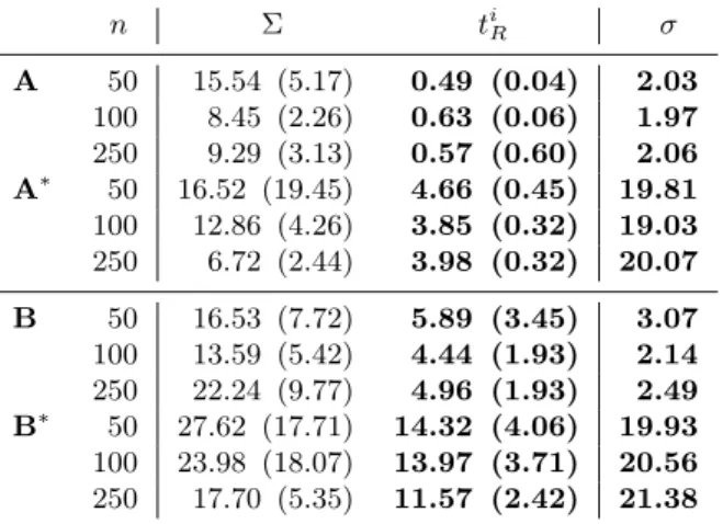
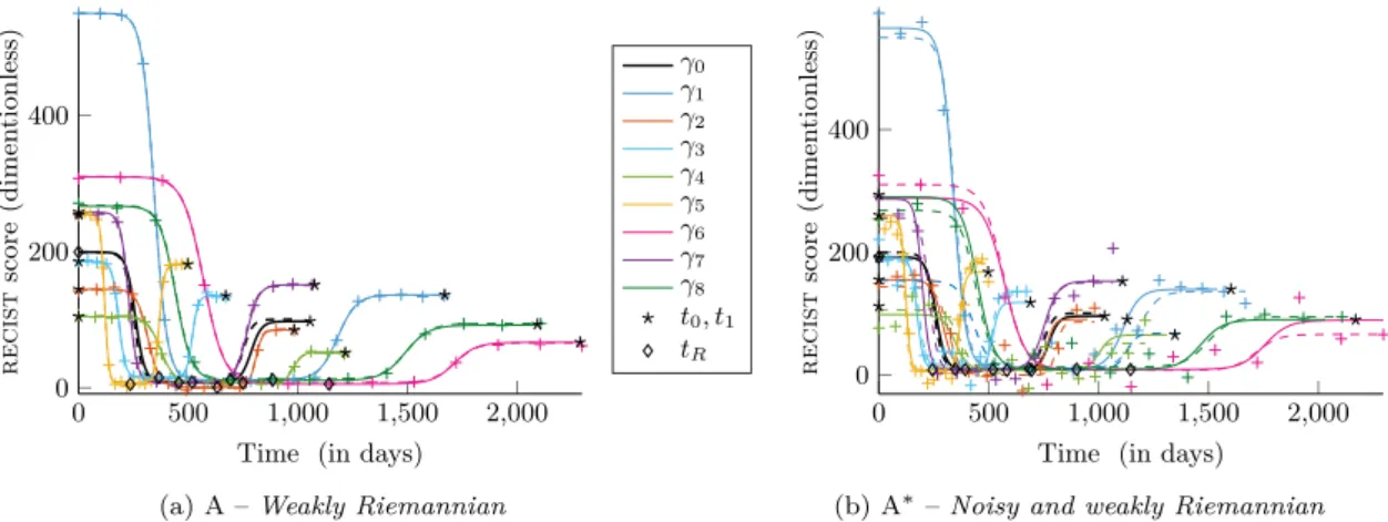
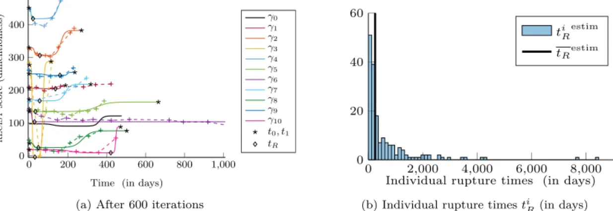
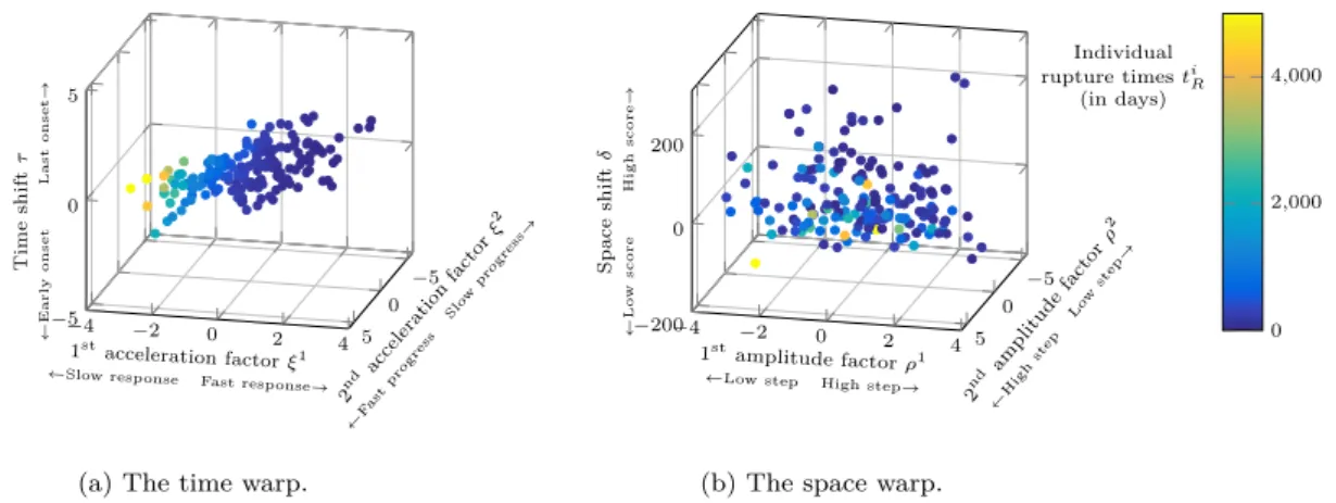
Due to the non-linearity of the model, we use the Stochastic Approximation Expectation- Maximization algorithm to estimate the model parameters.. Experiments on syn- thetic

De Vries makes a strong case for important structural changes in Europe during the ªrst half of the century, arguing persuasively for the existence, and importance, of crisis in