Time-varying delay systems and 1-D hyperbolic equations, Harmonic transfer function and nonlinear electric circuits

(1)

HAL Id: tel-03105344

https://hal.archives-ouvertes.fr/tel-03105344

Submitted on 11 Jan 2021

HAL is a multi-disciplinary open access archive for the deposit and dissemination of sci-entific research documents, whether they are pub-lished or not. The documents may come from teaching and research institutions in France or abroad, or from public or private research centers.

L’archive ouverte pluridisciplinaire HAL, est destinée au dépôt et à la diffusion de documents scientifiques de niveau recherche, publiés ou non, émanant des établissements d’enseignement et de recherche français ou étrangers, des laboratoires publics ou privés.

Time-varying delay systems and 1-D hyperbolic

equations, Harmonic transfer function and nonlinear

electric circuits

Sébastien Fueyo

To cite this version:

Sébastien Fueyo. Time-varying delay systems and 1-D hyperbolic equations, Harmonic transfer func-tion and nonlinear electric circuits. Mathematics [math]. Université Cote d’Azur, 2020. English. �tel-03105344�

(2)

Systèmes à retard instationnaires et EDP hyperboliques 1-D

instationnaires, fonctions de transfert harmoniques et

circuits électriques non-linéaires

présentée et soutenue publiquement par

Sébastien Fueyo

En vue d’obtenir le grade de

Docteur en Sciences

de l’Université Côte d’Azur Discipline : Mathématique

Equipe FACTAS et MCTAO - Inria Sophia Antipolis-Méditerranée Thèse co-dirigée par

Laurent BARATCHART et

Jean-Baptiste POMET Soutenue le 30 octobre 2020

Devant le jury composé des directeurs de thèse et de :

Yacine Chitour Professeur Université Paris-Saclay Rapporteur

Jonathan R. Partington Professeur University of Leeds (Royaume Uni) Rapporteur Birgit Jacob Professeur Bergische Universität Wuppertal (Allemagne) Examinateur Hoài-Minh Nguyên Professeur Ecole Polytechnique Fédérale de Lausane (Suisse) Examinateur Almudena Suárez Professeur Universidad de Cantabria (Santander, Espagne) Examinateur

Marius Tucznak Professeur Université de Bordeaux Examinateur

(3)

(4)

Time-varying delay systems and 1-D hyperbolic

equations, Harmonic transfer function and

(5)

(6)

Résumé /Abstract

Résumé

Les amplificateurs contiennent des composants linéaires passifs, ainsi que non-linéaires actifs, qui peuvent tous être décrits par un nombre fini de variables d’état; ils contiennent aussi des lignes de transmission, généralement modélisées par des équations aux dérivées partielles 1-D hyperboliques comme les équations du Télégraphe sans perte qui rendent l’espace d’état de dimension infinie. En utilisant une forme intégrée des équations du Télégraphe, on obtient un modèle composé d’équations aux différence retardées et d’équations différentielles. Considérant une trajectoire périodique qui s’établit dans l’amplificateur à cause d’un signal périodique forçant, la thèse vise à caractériser la stabilité locale d’une telle trajectoire périodique. En utilisant une approximation de premier ordre, cela se réduit à étudier la stabilité exponentielle du système linéaire périodique temporel obtenu par linéarisation autour de la solution périodique, et qui est un réseau d’équations aux différences retardées dont les conditions aux limites sont couplé par des équations différentielles. La stabilité de ce type d’équations est fortement corrélée avec la stabilité d’un système périodique aux différences linéaires (via un argument de perturbation compacte). La thèse établit alors des conditions pour garantir la stabilité des systèmes retardés périodiques linéaires.

En raison du nombre énorme de composants électroniques, il est connu dans les livres d’ingénierie électronique que la stabilité ne peut pas se déterminer directement à partir du système linéarisée. Ainsi pour étudier les propriétés de stabilité du système linéarisé précédent, une famille de systèmes entrées-sorties est construite, obtenue en perturbant le système linéarisé par un petit courant i à un nœud du circuit et en observant la perturbation résultante de tension v entre deux nœuds. Via un développement de Fourier, la stabilité se ramène à étudier les singularités de la fonction de transfert harmonique (FTH) qui est une matrice infinie dépendant d’une variable complexe et à valeur banachique. Sous des hypothèses de dissipation à haute fréquence qui sont toujours vérifiées pour les amplificateurs, la thèse montre alors que la FTH possède au plus des pôles dans un demi plan droit complexe contenant strictement l’axe imaginaire. Ces pôles sont en particulier les logarithmes d’une famille finie de nombre complexe, et sous une hypothèse de contrôlabilité et d’observabilité, la solution périodique est localement stable si et seulement si la FTH n’a pas de poles dans le demi-plan droit complexe.

Mots clés: Système retardé à temps variant, Système hyperbolique 1-D à temps variant, Fonction de transfert harmonique, Stabilité, Circuits électriques.

(7)

6 Résumé /Abstract

Abstract

Amplifiers contain linear, passive components as well as nonlinear, active ones, all of which can be described by finitely many state variables; but they also contain transmission lines, typically modeled by simple hyperbolic Partial Differential Equations (PDE) like lossless telegrapher equations, that make the global state space of the circuit infinite-dimensional. Using an integrated form of telegraphers equations, one obtains a model comprised of delay difference and differential equations. Using first order approximation, this reduces to exponential stability of the time-periodic linear system obtained by linearizing around the periodic solution, which is a network of delay difference equations whose boundary conditions are coupled by differential equations. The stability of this kind of equation is strongly correlated with the stability of a periodic linear difference delay system (via a compact perturbation argument). The thesis then establishes conditions to guarantee the

stability of periodic difference delay system systems.

Due to the huge number of electronic components, it is known in electronic engineering textbooks that stability cannot be determined directly from the linearized system. To study the stability properties of the previously-described linearized system, one constructs a family of input-output systems, obtained by perturbing the linearized system by a small current i at some node of the circuit and observing the resulting perturbation of the voltage v between two nodes. Via a Fourier development, stability is studied through the singularities of the harmonic transfer function (HTF) which is an infinite matrix depending on a complex variable with Banach value. Under high frequency dissipativity assumption, which are always verified for amplifiers, the HTF has at most poles in a complex right half-plane containing strictly the imaginary axis. These poles are in particular the logarithms of a finite family of complex numbers, and under an assumption of controllability and observability, the periodic solution is locally stable if and only if the HTF has no poles in the complex right half-plane.

Keywords: Time-varying difference delay equations, Time-varying 1-D hyperbolic systems, Harmonic transfer function, Stability, electric circuit.

(8)

Remerciement

Je voudrais tout d’abord remercier mes directeurs de thèse. La culture scientifique, et non scientifique, de Laurent Baratchart ont été et sont une grande source d’inspiration, bien que j’ai et ai eu besoin souvent d’un delai de trois mois pour comprendre ses idées profondes. Son éthique scientifique, sa qualité rédactionnelle et ses idées originales ont su guidé mon travail de thèse. Le sens pédagogique de Jean-Baptiste Pomet et son sens de la phrase juste m’ont permis de mieux exprimer mes idées mathématiques.

Je remercie Yacine Chitour et Jonathan Partington d’avoir accepté de rapporter cette thèse. Je les remercie pour leurs suggestions qui ont aidé à améliorer la qualité de ce manuscrit.

Je remercie Marius Tucznak d’avoir accepté de présider mon jury, ainsi que Birgit Jacob, Hoài-Minh Nguyên, Almudena Suárez et Adam Cooman d’y avoir participé.

Concernant mon travail de thèse, il doit également beaucoup à Gilles Lebeau et son expertise précieuse pour la stabilité des EDP hyperboliques.

Tout au long de ces quatre années, l’équipe FACTAS (feu APICS) a fourni des conditions de travail idéales. Si j’étais le guide Gault et Millau, je recommanderais chaudement d’aller faire un tour à la table de cette équipe aux heures de déjeuner, tout en vous invitant à réviser la situation géopolitique du Guatemala sous peine d’être possiblement perdu pendant la discussion. Je remercie plus personnellement Fabien et son sens de l’humour (ainsi qu’une pensée émue pour la salade de pomme de terre qu’il ne pourra pas manger à Noël cette année), Juliette pour les innombrables pauses cafés ainsi que sa dextérité pour dompter la machine infernale, Martine pour sa gentillesse (je n’en écrirais pas trop ici car l’octet pollue), Sylvain pour ses qualités pédagogiques et sa capacité à résoudre tout problème informatique en un temps record, ainsi que Marie-Line pour m’avoir aidé dans les taches administratives parfois abstruses.

Je remercie également l’équipe McTAO, même si l’incompatibilité du fuseau horaire concernant l’heure du déjeuner m’a amené à moins les côtoyer que l’équipe FACTAS. Je remercie Jean-Baptiste, dît le jeune, qui j’espère notera la propreté du bureau que j’ai laissé derrière moi, Lamberto et sa chaleurosité (en espérant que ce mot entre un jour dans le dictionnaire!) toute italienne, ainsi que Laetitia que j’ai moins connu.

Passons maintenant aux doctorants et posdoctorants que j’ai été ammené à côtoyer! David le Murcian aux problèmes, et aux solutions également, improbables. Adam le Flamand jovial avec qui j’avais un accord tacite: il m’expliquait l’électronique et les lignes de transmission tant que je lui donnais mon dessert à manger, ce qui tombait bien car je ne comprenais pas les lignes de transmission et lui oui, et je n’avais plus faim alors que lui était affamé. Gibin qui m’aura permis de situer la région de Kerala en Inde. Yacine qui a été un collègue de bureau fort agréable et qui m’a permis de retrouver la joie de jouer aux échecs (et de souvent perdre!). Ainsi que les inombrables doctorants qui sont passés de façon plus éphémères comme Pauline, Axel, Lucie, Sofya, Vanna Lisa et Christos. Je souhaite bonne chance pour leurs fins de thèse à Paul le constructeur d’abris pour

(9)

8 Remerciement

tortue, Masimba qui va bientôt parler un français impeccable et Alesia en espérant que la situation de son pays s’améliore.

J’ai aussi une pensée pour tous les professeurs ayant marqués mon cursus scolaire. Tout d’abord je pense à M.Delgendre professeur d’histoire-géographie au collège La Guicharde et Arnaud Beaumont professeur de philosophie, et je remercie ces derniers pour la curiosité intellectuelle qu’ils m’ont transmise. Ensuite je pense aux enseignants que j’ai eu lors de ma préparation à l’agrégation à Marseille et qui ont été décisifs notamment Pierre Bousquet, Franck Boyer et Brigitte Mossé.

Je remercie également Claudine Chaouiya et Elisabeth Remy de m’avoir initié il y a maintenant fort longtemps aux systèmes dynamiques discrets, et en espérant un jour pouvoir retravailler avec vous sur ces sujets.

Enfin, et plus personnellement, je remercie ma maman de m’avoir élevée seule et d’avoir toujours tout fait pour moi. Merci à mon oncle (dit Parrain ou Tonton Grumeau) et ma tante (dit Tatie Sylvie) pour m’avoir accueilli en leur maison en 2014 et sans qui ce travail n’aurait pas existé. Je remercie mon papa, même si les relations n’ont jamais été simple, d’être à nouveau prêt de moi.

Mes dernières pensées iront à ceux qui ne sont plus de ce monde. Papy Jo et Mamie Lucie, mes grands-parents. William, mon ami qui était le seul témoin de ma profonde incompréhension du théorème de Banach-Steinhaus.

(10)

List of figures

1.1 Elementary dipoles . . . 27

1.2 Controlled current source. . . 28

2.1 Nonlinear circuit containing a lossless transmission line. . . 42

2.2 Linearised circuit around the periodic solution disturbed by a current u . . . 43

3.1 A m multiport . . . 69

3.2 Model of a transmission line . . . 70

5.1 A graph that induces coupling boundary conditions for (5.1) with N = 4. . . . 105

6.1 A m multiport . . . 144

6.2 Two realistic models of a linearised diode . . . 147

(15)

(16)

Introduction

Motivation, Computer Assisted Design for circuits

This work applies to more general active circuits than amplifiers, like pure oscillators, but we restrict the motivations to amplifiers for simplicity. An ideal amplifier would be an active circuit that outputs exactly the input signal multiplied by some gain that does not depend on the signal. In practice, amplifier design consists in proposing a circuit, made of available elementary elements, so as to obtain a gain that does not vary too much when the input belongs to some class of signals. The available elementary elements are of three sorts:

• passive components: resistors, capacities and inductances,

• active nonlinear components: diodes and transistors (fed by an external power source), • lines that induce some delay effect, negligible at low frequencies.

The specification of an amplifier is always given in terms of a “frequency response”, i.e. the output occurring for sinusoidal input signals of all possible frequencies. The purpose of computer aided design (CAD) tools is to compute this frequency response for a given circuit design proposed by the user. For RLC circuits, this may be readily computed, even analytically, possibly using computer algebra if the number of components is very large. For more complex ones, where the response of some elements may be available numerically only, specialised tools are needed, (see e.g. [Key]). They rely on a dynamical model of the circuit, obtained from the models of all components, and compute numerically a forced periodic solution of this dynamical system under periodic excitation, through a numerical method, often referred to as “Harmonic Balance”, that we briefly describe in Section 1.2.

There is substantial recent literature on the subject in Electronic Engineering, see for instance [Kun06, SQ02,Sua09], because this is important for circuit design. Knowing whether the computed periodic solution corresponds to the steady state response to periodic excitation that will be observed in real life is obviously very important. Two related points are commonly raised. First, there may be more than one possible response to a given sinusoidal signal, at least for the mathematical/numerical model used by the CAD tool: it would be more correct to state that these tools compute one response. We do not investigate this point further. The second point is certainly more determining and has received a lot of attention: the stability of the computed response is not a priori guaranteed, and if the response happens to be unstable it will simply not be observed because it would occur only for very special initial conditions of inner variables of the circuit, that are in practice never exactly achieved. On the contrary, with the additional information that all the computed responses are stable, it would be granted that numerical tools predict the frequency response (at least if the basin of attraction is reasonably large in terms of the inner variables of the circuit, but we do not deal with this question here and consider local stability only, obviously necessary). Stability is by no means a straightforward side-result of the estimation of the response: it may happen that a

(17)

16 Introduction

computed response is unstable (although the numerical process converged). Determining stability of the computed response is hence crucial, it has retained a lot of attention and some methods are indeed even implemented [STA,CSO+₁₆_,_Sua15_,_SQ02_].

The initial motivation of this thesis is the mathematical framework to determine stability of a given response as computed by these CAD tools. We hope to provide some mathematical insight.

The stability question

Let us now say a work about the model of the circuit, examine what the response for a fixed harmonic/periodic/sinusoidal signal is, and state the stability question more precisely. Without transmission lines, the equations of a circuit composed of the above mentioned elementary components are given by a set of ordinary differential equations (ODEs), hence a model with an finite dimensional state; this case is reviewed in Chapter1. Taking the lines into account, as in most of this thesis, leads, on the contrary, to a model with an infinite dimensional state, containing for instance currents and voltages distributed along the lines, the model is of a more complex nature, it is a set of hyperbolic partial differential equations (PDEs) modeling the lines, coupled by ODEs through their boundary conditions; when the PDEs are lossless Telegrapher’s equations, as always assumed here, the model can also, thanks to explicit integration of the PDEs, be viewed as a “hybrid” system including delay equations and differential equations (see (1) below), the state being then more abstract.

For a given periodic input signal, the amplifier, including the excitation by that signal, can be seen as a complex periodic time-varying dynamical system, whose state is all the currents and voltages, possibly distributed in the lines. We are interested in periodic solutions of this dynamical system, with the same period as the input. As mentioned above, there might be more than one; without discussing existence or uniqueness, we assume that we are provided with a periodic solution,

i.e. a possible response of the amplifier, obtained numerically, and we need to decide on its stability.

Recall that this stability (i.e. the property that starting from initial conditions close to the solution leads to remaining close and even to converge to the solution) is certainly a necessary condition for this solution to be observed in reality: without stability, the observed behaviour may be an escape to high currents and burn, or convergence to another periodic solution, or actually more chaotic behavior.

A classical step to determine stability is to linearise the dynamical system around the now known periodic solution, obtaining a periodic time-varying linear dynamical system, whose (strict exponential) stability amounts to local stability of the periodic solution. This stability could be determined by computing Floquet exponents, or the spectrum of the discrete flow pushing the state one period ahead, but these computations are out of reach, because of the great number of transmission lines and because the periodic solution we linearise around is only known numerically. The way around is to analyse this stability in an indirect manner, through an auxiliary linear input-output system that relates a fictitious input to a fictitious output and whose dynamics (drift) is the considered time-varying linear system; the input is for instance a current added between two points and the output the measurement of some voltage, in the linearised circuit. The point that makes this construction relevant is that this fictitious input-output system can be made real for the CAD tool, and this tool can compute its frequency response, that in turn may be used to assess the desired stability.

To describe the way one uses this frequency response, let us make, for a while, a simplifying assumption, that occurs for instance if the periodic signal to be amplified is the zero signal and hence the periodic solution is simply an equilibrium point: we assume in this paragraph that the the linear input-output system is time-invariant. Its frequency response is then simply the value on the imaginary axis of its transfer function. Determining stability from the knowledge of the transfer

(18)

Introduction 17 function on the imaginary axis led to a large literature from a theoretical or numerical viewpoint. It is well known that, provided that the auxiliary input-output system is controllable and observable, the spectrum of the operator defining the linear dynamics is the locus of singularities of the transfer function, so that local exponential stability of the origin for the linear dynamical system occurs if and only if the transfer function has no singularity in the right half plane (see [PW97]). It has been proven in [BCC+₁₈_{] that the transfer function is meromorphic for such time-invariant systems, even} in the presence of transmission lines; this legitimates the use of rational approximation to determine the possible unstable poles, all the more so as the same reference also proves that there are at most a finite number of such poles in the right half plane if the system is “dissipative at high frequency”, which is the case of any realistic circuit. Rational approximation methods are not in the scope of this thesis, we only make a rough sketch in Section 1.5 (Chapter 1), but we retain the principle that a method that amounts to find poles of a function in a domain where it is meromorphic is feasible. Modulo this principle, one now sees how to determine stability in the case of an equilibrium point, leading to a time-invariant linear approximation. The two ingredients that make this method (use of an auxiliary input-ouptut system, estimation of the transfer function of the imaginary axis, rational approximation) workable are on the one hand that stability is captured by the location of the singularities of the transfer function and on the other hand that the part of the singularities that have to be identified to decide stability are poles, so that rational approximation is relevant.

Let us go back to the more general case of a periodic excitation creating a periodic solution, leading to a periodic time-varying linear approximation and an auxiliary periodic time-varying linear input-output system. There is a generalisation of the concept of transfer function to these latter systems, it is called harmonic transfer function (further denoted HTF). It was introduced rather recently [Wer90] in the context of circuits, it is not very well known in the control theory community, probably because time-varying linear systems have retained little attention. Since it is a central object in the thesis, we define it with some care, for finite-dimensional systems (i.e. neglecting transmission lines) in Chapter 1, for an example (with lines) that we treat extensively in Chapter 2, and in general in Chapter6. Its definition is based on the Fourier development of the system. The HTF is a more sophisticated object than the usual transfer function: instead of a single function of the complex variable, it is an infinite matrix with square integrable lines, whose entries are analytic function of a complex variable, analytic in some domain of the complex plane, or it can also be seen as an operator valued (operators l2_{(Z) → l}2_{(Z)) function of the complex variable. The}

values on the imaginary axis of the coefficients of this infinite matrix also derive from the frequency response computed by the CAD tool. This suggests a similar route as the one we just described for time-invariant systems. However, to complete the analysis, the two “ingredients” mentioned at the end of the previous paragraph have to be provided in the case of periodic system too. On the one hand, we have to link the local stability of the periodic solution with the singularities of the harmonic transfer function, or of the entries of the infinite matrix than encodes it. On the other hand, we have to determine what the structure of the HTF is and wether this operator is meromorphic or not on the domain that matters for stability, namely the right-half plane, in order to apply, for instance to a few entries of the infinite matrix defining the HTF, rational approximation algorithms as discussed in Section1.5. The arguments given in [BCC+₁₈_{], based on complex valued} function analysis, are not sufficient anymore when we consider the harmonic transfer function; in fact, as mentioned above, the HTF takes its values in a complex Banach space and the theory for these objects is less tractable than for complex functions. Solving the problem will lead us through the theory of the delay systems, functional analysis via a compact perturbation argument, the Lyapunov functions and a constant back and forth between time-domain and frequency-domain.

(19)

18 Introduction

Mathematical point of view, models, summary of contributions

Let us move to a more mathematical viewpoint to describe our work in more details. Each lossless transmission line is modeled, in this thesis, by a Telegrapher’s equation. An amplifier is a directed graph where the edges are the lossless transmission lines and the nodes are composed of the active nonlinear components and the passive components. Under the assumption that at each node we can express all the currents and voltages in function of the voltages of the condensators, the currents of the inductors and the currents of the lines which arrive at this node, the resolved form of these 1-D hyperbolic equations leads to the following type of periodic nonlinear “hybrid” delay system (this is detailed in Chapter 3):

( _dx(t)

dt = f(t, x(t), y(t), y(t − τ1), · · · , y(t − τN))

y(t) = g(t, y(t − τ1), · · · , y(t − τN), x(t))

(1) where f and g are obtained through the implicit function theorem from implicit equations, we neglect this difficulty and assume these maps reasonably smooth. This assumption is systematically made in electronic engineering, the justification is not immediate for singularities in the equations may occur, see for instance [Sma72], but it seems that algorithms in the CAD tools would not manage to find periodic solutions going through these singularities.

We assume that System (1) admits a periodic solution (x(t), y(t)) and we are interested in local stability of this periodic solution. Linearising System (1) around this periodic solution yields a linear time-varying system:

       dx(t) dt = A1(t)x(t) + N P i=0 B_i1(t)y(t − τi), y(t) = PN i=1 B_i2(t)y(t − τi) + A2(t)x(t), (2)

where the smoothness of the functions of time depend on the smoothness of f and g and on the smoothness of the periodic solution.

Under adequate smoothness assumptions, we prove in Chapter 6 that the periodic solution (x(t), y(t)) of System (1) is locally stable if the origin of the linearised system (2) is exponentially stable. Thus local stability is reduced to exponential stability of the linearised system. We also prove that we have this exponential stability if and only if the monodromy operator of System (2) has its spectrum strictly inside the unit disk, the monodromy operator being the operator which integrates the solution one period ahead. These preliminary results are classical but needed technical adaptation. The core of the thesis is devoted to describing this spectrum in relation with the singularities of the HTF (Harmonic Transfer function, introduced above) of some input-ouptput system. Let us keep in mind that the spectrum of an operator defined on an infinite dimensional Banach space is usually more complicated than a finite set of eigenvalues.

One step in that direction is to consider the “high frequency limit” of System (2), that puts to zero the x component and leads to the following periodic linear difference delay system:

z(t) =

N

X

i=1

B_i2(t)z(t − τi). (3)

For circuits, the behavior of the system at high frequency means that, the condensators become wires and the inductors become open switches. This is of help for two reasons.

• On the one hand, we prove (see Chapters2and6) that the monodromy operator of System (2) is a compact perturbation of the monodromy operator of System (3). So, if one proves

(20)

Introduction 19 exponential stability of (3), i.e. if one proves that the spectrum of the monodromy operator of (3) is contained in a disk of radius strictly less than 1, this establishes that the spectrum of the monodromy operator of System (2) is composed of a finite number of eigenvalues outside a disk with radius strictly less than one and some part of that disk, that we do not have to describe because it does not impair stability.

• On the other hand, exponential stability of difference delay systems of the type (3) is studied in a detailed manner in Chapters 4and5. The literature on such equations is really scarce in the time-dependent case, we believe that the material in these two chapters has an interest beyond microwave circuits, but in any case they prove that exponential stability holds for these systems, i.e. for (3), under a passivity property that is always, implicitely or explictely, assumed in electrical engineering.

The fact that any real life circuit, like an amplifier, is passive, or dissipative, at high frequency roughly means that, although active, the circuit does not inject energy in high frequency enough signals. When making a “theoretical” circuit out of ideal diodes, transistors, capacitors, inductors and lines, one may easily come up with a circuit that does not have this property, hence is not “real life”. Assuming this property for our models amount to not forget to add some small capacities or inductances or resistances here and there, to make “ideal” elements more real. Dissipativity is also a well known idea in mathematics to study the stability of the systems [BC16,Wil72,BLME07,TGTN+₀₇_,_Wil13_].

Since high frequency passivity is always assumed, this closes the needed description of the unstable part of the spectrum of the monodromy operator of (2), now known to be composed of isolated eigenvalues only.

The last point needed in the process, and addressed by the thesis, is to link the unstable part of the spectrum of the monodromy operator with the unstable singularities of the HTF of the input-ouptut system obtained by disturbing the circuit represented by System (3) with a current

uand observe the voltage response v1 at some node; the resulting input-output system is of the form:

                 dx(t) dt = A1(t)x(t) + N P i=0 B1_i(t)y(t − τi) + C1(t)u(t) y(t) = PN i=1 B2 i(t)y(t − τi) + A2(t)x(t) + C2(t)u(t) v1(t) = N P i=0 B_i3(t)y(t − τi) + A3(t)x(t) + C3(t)u(t), (4)

for suitable periodic time varying matrices B3

i(.), A3(.), C1(.), C2(.), C3(.).

The development of the matrices depending periodically on time in System (4) into Fourier series and the Laplace transform allow us to better describe the concept of the HTF: it can be defined as the infinite matrix H(·) function of the complex variable s such that the input and the output are linked (modulo transients) by

          ... L{v₁}(s + iω₀) L{v₁}(s) L{v1}(s − iω0) ...           = H(s)           ... L{u}(s + iω₀) L{u}(s) L{u}(s − iω0) ...           , (5)

(21)

20 Introduction

where ω0 = 2π/T denotes the proper frequency of the system and L{·} denotes the Laplace

transform: L{v1}(s) := Z +∞ 0 e−stv1(t)dt , L{u}(s) := Z +∞ 0 e−stu(t)dt . (6)

The definition of the HTF will be re-stated and made more precise in Chapters 1,2 and6.

Let us briefly state how this thesis links the HTF of System (4) with the monodromy operator of System (2). Under the stability at high frequency of the amplifier, we are able to prove that the HTF is meromorphic in some “extended” right half-plane {z ∈ C, <(z) > −α} with α positive, and that all its poles in that half plane are logarithms of eigenvalues of the monodromy operator of System (2). This justifies the paradigm that under the stability at high frequency, all unstable singularities are poles. This is proved into details on a class of examples in Chapter 2 (on this class of example, system (3) reads z(t) = a z(t − τ) with z scalar real, τ > 0 and |a| < 1 so that its stability is not the major problem) and in Chapter 6for general systems (4). A difficult unsolved problem is to tell in advance which logarithms will indeed be singularities and which entries of the infinite matris H(·) do carry these singularities. Partial results are given. The notion of singularities of this infinite matrix, or of this operator valued function, is subtle.

We describe our contributions in a more detailed way, chapter by chapter, in the next “Plan and contributions of the thesis”.

(22)

Plan and contribution of the thesis

Generalities

Chapter 1is an overview of the knowledge concerning the Harmonic Balance (HB) techniques, the

Harmonic Transfer Function (HTF) and the link with the local stability for the circuits modeled by nonlinear ordinary differential equations ([Wer90, Lou14, Sua09, Hal69]). Chapter 1establishes the major ideas to study the periodic systems in finite dimension:

• the Floquet theory which sa ys that a linear periodic differential equation is equivalent to a constant differential equation modulo a periodic change of basis.

• the fact that the local stability is given by the spectrum of the monodromy operator, i.e. the operator solution that we integrate after one period.

• the variation of constant formula which permits to express the solution of a periodic linear differential equation disturbed by a pertubation in function of the periodic linear differential equation itself.

• the Harmonic Transfer Function is an operator valued analytic map, where the values are the continuous operator from l2_{(Z) to l}2_{(Z) with l}2_{(Z) denoting the square summable series.}

• the singularities of the Harmonic transfer function are at most the logarithm of the eigenvalues of the monodromy operator.

• under the classical controllability and observability assumption, if the Harmonic Transfer Function is analytic in the closed right half plane then the periodic solution is locally stable. Chapter 2 is devoted to the study of a simple circuit which possesses only one lossless

transmission line. This circuit reduces to a nonlinear neutral differential equation and we follow the theory that we can find in [HVL93]. The theory stated in [HVL93] deals with the continuous solutions (space C0_{) for the neutral differential system. In fact, the theory can be generalized for}

the square integrable functions (L2 _{space) and for the absolutely continuous functions with a square}

integrable derivative (W1

2 space). The necessity to use the square integrable functions comes from

the fact that the harmonic transfer function is viewed as an infinite matrix defined on the space of the square summable series. The absolutely continuous function with square integrable derivative occurs because, via the resolution of a first kind Volterra equation, the system is controllable on this space with a square integrable function; i.e. each element of W1

2 can be reached with an element

of L2_{. The semigroup theory, a compact perturbation argument and the variation of constant}

formula permit to prove that the HTF is a meromorphic operator in the closed right half plane where the poles are the complex logarithm of a finite number of complex numbers, and if the HTF is holomorphic in the closed right half plane then the periodic solution is locally stable. Moreover if we add observability assumptions, the HTF has essential singularities view as a Banach valued operator in the left half plane when the delay and the period are not commensurable.

(23)

22 Plan and contribution of the thesis

Chapter 3 reduces the network of lossless Telegrapher’s equations with nonlinear differential

boundaries to difference differential equations coupled with nonlinear difference equations. The result is not new but it seems difficult to find a proper reference in the literature. Moreover, this reduction is allowed under the assumption that at each nodes of the network, we can express all the voltages and currents of this node in function of the voltage of the condensators, the current of the inductors and the current at the end of the lines connected to this node.

Linear time-variant difference delay systems

Chapters 4and5 focus on the stability of the linear time-varying difference delay equations. The literature is relatively large for linear time-invariant delay equations ([CH70,Hen74,HVL93]) but becomes sparse when the equations are time dependent, where the most complete study can be found in [CMS16].

Chapter 4 gives a sufficient and necessary stability condition for a periodic linear difference

delay system with continuous Hölder derivative.

The proof of the sufficiency follows the ideas of [Hen74,BC63]. More precisely, we establish a variation of constant formula which permits to express all the solutions of the periodic difference delay system in function of one so called fundamental solution and the initial data. The use of the Fourier development and the Laplace transform allow us to bound exponentially the variation of the fundamental solution and we conclude the exponential stability of the system. Contrary to the time-invariant case, the difficulties come from:

• we have to invert an analytic almost periodic operator a Banach space on a vertical strip and the theory of the analytic almost periodic complex function does not apply anymore ([Bes54]), • we have to justify the swapping between the series coming from the Fourier developpment

and the integral coming from the Laplace transform.

The proof of the necessity used in [Hen74,BC63] uses the spectral semigroup properties for time-invariant difference delay systems. In our case we cannot follow this path because the periodicity. However we are able to prove the necessity of our stability condition with the use of an input-output system.

The result is applied to the 1-D hyperbolic equations with continuous Hölder derivative bound-aries, equations which are a little more general than the lossless Telegrapher’s equations. We also give some conjectures for different periodic delay systems, systems more general than the periodic difference delay system with a finite number of delays that we considered in this chapter.

Chapter 5 undertake the study of the time-varying (not necessarily periodic) linear difference

delay system which comes from a network of lossless Telegrapher’s equations. When the system is time-invariant, we can find all the classic stability results in [BC16]. The idea of this chapter is to exploit the equivalence between the L2 _{exponential stability (for the square integrable solution) and}

the C0 _{exponential stability (for the continuous solution). This result can be found in [}_CMS16_{], but}

we hope to prove in a slight easier way the same result in Chapter5. Assuming that the network dissipates energy at each node, we utilise a Lyapunov function to prove the L2 _{exponential stability}

and so the C0 _{exponential stability. In particular, the reasonning permits to give a stability criteria}

for the subclass of difference delay system which have the column disjoint.

Hybrid delay systems, harmonic transfer function and application to the circuits containing lossless transmission lines

Chapter 6 deals with generalities concerning the nonlinear hybrid delay equations, i.e. difference

(24)

generaliza-Plan and contribution of the thesis 23 tions obtained in the periodic neutral differential case in Chapter 2; the results are based on the establishment of a variation of a constant formula and a compact perturbation argument.

These theoretical results about delay systems are applied to nonlinear electric circuits containing lossless transmission lines. Under the assumption of the dissipativity at high frequency of each components of the circuit, we are able to prove that the harmonic transfer function is meromorphic in the closed right half plane and the poles are the logarithm of a finite number of complex numbers. Moreover, under controllability and observability assumptions, if the harmonic transfer function is analytic in the closed right half plane then the periodic solution is locally stable.

The outcomes of this chapter legitimate the harmonic balance techniques and the search of poles in the closed right half plane via meromorphic or rational approximations under the rather weak assumption of the dissipativity at high frequency of the circuit.

(25)

(26)

Chapter

1

Theory of the circuits modeled by

ordinary differential equations

Although the thesis is devoted to active circuits in which the effect of transmission lines is important, we start with a chapter on the case where this effect can be neglected. The resulting models are ordinary differential equations rather than a coupling of these with propagation equations, as described in Chapter 2for an example and Chapter3and further in general. In this simpler setting, we review here known facts and ideas, but we also show that the mathematical treatment still contains some challenges and open questions.

The considered circuits contain resistors, diodes (introducing nonlinearities), capacitors and inductors, as well as a periodic generator that represents a (periodic) signal to be amplified.The “amplifying” energy is brought by the diodes, that make the circuit active (non conservative).

We first recall how to obtain the equations of such a circuit. We then show that it is reasonable to assume that these equations have a periodic solution and describe a practical method to compute an approximation of this solution and of the linearized equations around this solution; the goal is to determine whether this periodic solution is stable.

Stability of this periodic solution is given by (global) exponential stability of the origin for the linear time-varying ordinary differential equation obtained by linearizing around the periodic solution. The most practical way to decide numerically on this stability is to generate the frequency response of a linear time-varying input-output system obtained by adding a perturbation to the linearized circuit, produced by an artificial additionnal current in some branch and imagining the measure of (for instance) a voltage between two nodes; there is some freedom in chosing this perturbation and this measure.

We describe briefly this process and the resulting linear time-varying input-output system, and then proceed to introduce the notion of harmonic transfer function, a generalisation of the well-known transfer function in the time-invariant case, that is not so classical and plays an important role in the thesis; it is more sophisticated than the transfer function: it is an operator valued (rather than scalar or matrix-valued) function of the complex variable. We discuss the relation between the singularities of this harmonic transfer function and exponential stability of the above mentionned time-varying linear ordinary differential equation. We prove that, if the perturbation and measure have been chosen so that the input-output system enjoys controllability and observability properties, the zero solution of the linear time-varying ordinary differential equation is exponentially stable if and only if the harmonic transfer function is holomorphic in the right half plane. Since it can be proved to be meromorphic in general, this justifies existing methods that apply rational approximation to a finite number of values of the frequency response of the input-output system (computed by Harmonic Balance methods) to locate poles. Here a discussion takes place on the fact that one only locates poles of coefficients in a Fourrier expansion of the Harmonic Transfer Function and not of the Harmonic Transfer Function as an operator value function. We also discuss rational approximation in this context.

(27)

26 Chapter 1. Theory of the circuits modeled by ordinary differential equations

1.1 Equations in finite dimension

We consider in this chapter the simplest nonlinear circuits that we can have, ie a circuit made of with two kind of electronic components : dipoles (inductors, capacitors, resistors and diodes) and transistors. More precisely :

i. A dipole, also called a branch [CC98], is an electronic box with 2 terminals, labeled 1, 2, such that the current through the box, oriented from 1 to 2, is related to the potentials V1, V2 at

the terminals by a linear, nonlinear or differential form. Elementary dipoles considered in this thesis are the following (see Figure 1.1):

• Ideal resistor, with :

vr = Rir, (1.1)

where R > 0 and vr = V2− V1.

• Ideal inductor, with Ldil

dt = vl, L > 0, vl= V2− V1. • Ideal capacitor, with Cdvc

dt = ic, C > 0, vc= V2− V1. • Ideal diode with :

vd= f(id) (1.2)

where f is a function and vd= V2− V1. In a circuit with a periodic solution, the ideal

diode is often approximate by its linearization around the periodic trajectory which leads to the equation :

vd= R(t)id, (1.3)

where R(t) is a periodic function (possibly negative). • Ideal periodic voltage generator :

v(t) = p(t), (1.4)

where p(·) is a C∞_{periodic function and v = V} 2− V1.

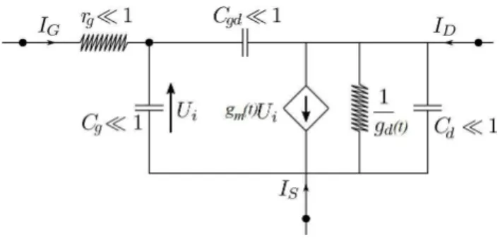
ii. A transistor is typically modeled by a controlled current source, usually combined with some

resistors and (non-linear) capacitors. After linearization the latter become ordinary capacitors, so we are left to describe the current sources and their linearization. A controlled current source has 3 terminals. When the transistor if a Field Effect Transistor (FET), these terminals are called gate, source, and drain, denoted respectively by G, S and D (see Figure1.2). Their behavior is described by a relation of the form :

iD = f(vGS, vDS) and iG= h(vGS, vDS), (1.5) where f, h are a non-linear real-valued function and vGS= VG− VS, vDS = VD− VS. As in the case of diodes, this simple model assumes no inductive nor capacitive effect, as f and

g only depends on vGS, vDS and not on their time derivatives, nor on the derivative of iD. Moreover the function f are increasing in both variables. Like the diode, we will often consider linearized transistor. In a circuit with a periodic solution, the ideal diode is often approximate by its linearization around the periodic trajectory which leads to the equation :

iD = gm(t)vGS+ gd(t)vDS and iG= ˜gm(t)vGS+ ˜gd(t)vDS, (1.6) where gm(t), gd(t), ˜gm(t) and ˜gm(t) are periodic functions. And gm(t) and gd(t) are strictly positive with the assumption on f.

(28)

1.1 Equations in finite dimension 27

(a) Resistor (b) Inductor

(c) Capacitor (d) Diode

(e) Periodic Voltage Generator

(29)

Figure 1.2 : Controlled current source.

The components defined in i and ii are put together to form a connected graph and we call this object a circuit. In a circuit, The link between the currents and the voltages in the circuit is given by the Kirchhoff law, ie the current arriving at each node is equal to the current leaving the node and the directed sum of the voltages around any closed loop is zero. We are interested to obtain the equations which governs the behavior of the circuit. Given a circuit, if we assume that all the voltages and all the currents of the circuit can be reconstructed from the knowledge of all the inductors’ currents and the capacitor’s voltages in the circuit thus the circuit is modeled by a nonsingular ordinary differential equation (result due to Brayon-Moser [BM64]). We have in the same way that if there exists some currents and some voltages which can give all the currents and voltages in the circuit, then the equations of the circuit are (possibly singular) ordinary differential equations (see chapter 10 of [HS74]). The more general result on the structure of the equation of such circuits has been proved by S. Smale ([Sma72]). He proved that these circuits are generically differential equation on a real submanifold.

Theorem 1.1 ([BM64]). Noting by abuse of notation all the inductors current i_l and all the

capacitors voltage vc of the circuit and assuming that all voltages and currents in the circuit can be

expressed by il and vc, then there exists two functions hl and hc such that :

       dil dt = hl(t, il, vc), dvc dt = hc(t, il, vc). (1.7)

Moreover hl or hc have the minimum regularity of the functions in equations (1.2) and (1.5). Theorem 1.2 ([Sma72]). Assuming that all voltages and currents in the circuit can be expressed

by x ∈ Rn _{which is a vector composed of some currents and voltages of the circuit (n is equal to the}

number of capacitors and inductors), then there exists two functions f and g such that : df(t, x(t))

dt = g(t, x(t)), (1.8)

Moreover f or g have the minimum regularity of the functions in equations (1.2) and (1.5). Remark 1.3. Theorems 1.1 and 1.2 stated here are a weaker version than the originals. In fact,

the function hl, hc, f and g are a particular structure (almost like an Hamiltonian System) but we

(30)

1.2 Harmonic Balance Approach to compute a periodic solution 29

1.2 Harmonic Balance Approach to compute a periodic solution

We consider an amplifier with a periodic signal which has to be amplified and we sketch how the electronic engineers, through the Harmonic Balance Approach, approximate the amplified signal. Our exposition of the method is a bit mathematical compared with standard electronic textbooks (see for instance [SQ03] and [Sua09]), which is why we start with the formal assumptions below that

make our account meaningful :

i. the circuit contains one and only one ideal periodic generator with a period T ,

ii. the functions (1.2) and (1.5) associated to the nonlinear elements of the circuit (ie diodes and transistors) are at least of class C4_,

iii. the assumption of Theorem 1.2is verified; hence,

df(t, x(t))

dt = g(t, x(t)), t ≥ 0, (1.9)

where f and g are at least C4 _{and T -periodic in their first variable, while x ∈ R}n _{is a vector} composed of certain currents and voltages in the circuit.

iv. the system (1.9) has a T -periodic solution x, forced by the periodic generator, which does not meet a singularity of (1.9), ie ∂2(t, x(t)) is invertible for all t real.

The periodic generator in assumption i. represents the signal which has to be amplified. Assumption

ii. is important because justifying the Harmonic Balance method mathematically requires some

smoothness. Assumption iii. allows us to express the equations of the amplifier. Among electronic engineers, it is commonly accepted that for almost all active circuit of interest there exists a periodic solution; i.e., that assumption iiii. holds. However, from a mathematical point of view, this is not obvious and it would be interesting to prove theorems on the generic existence of periodic solutions for such circuits. It has to be noted that under a kind of dissipativity assumption at high frequency (see equation (1.10) below), one can prove the desired existence via the Brouwer fixed-point theorem

:

Theorem 1.4. Denote (, ) (resp. || · ||) the scalar product (resp. Euclidean norm) on Rn. Assuming

that f(t, x(t)) = x(t) in the system (1.9) and that :

(x, g(t, x)) < 0, (1.10)

for all t real and all x such that ||x|| ≥ k for some fixed k > 0, then the system (1.9) admits at least

one periodic solution of period T .

Proof. The equation (1.10) permits to prove that all the solutions of the system (1.9) are bounded and then the Brouwer fixed-point theorem give the result (see [SC64] p.366).

The assumption (1.10) is always true for realistic circuits. In fact, the realistic diodes and transistors have capacitive and inductive effects and so have just resistive effects at high frequency. Hereafter we do not discuss further the existence of a periodic solution, and we take it for granted. The Harmonic Balance method seeks an approximation of a T -periodic solution to the system (1.9). However, surprisingly perhaps, there may exist periodic solutions to system (1.9) with a period different from T (see [CGM16]). It is clear that under our regularity assumptions, a periodic solution x is of class at least C3_.

Let us quickly go through the method to compute an estimate of a truncated Fourier series of the periodic solution, following loosely the exposition in [Sua09]. The idea of this method, called harmonic balance, is simple and can be summed up as :

(31)

• using the Laplace transform, we convert the time domain into the frequency domain, • we develop the periodic system in Fourier series and to truncate these series,

• we solve for the truncated Fourier coefficients using a numerical fixed point method. More precisely :

i. We note

ω0 := 2π

T (1.11)

the proper frequency of the system. We take the Laplace transform of the system (1.9) evaluated in x for s ∈ C with strictly positive real part :

sL{f(t, x(t))}(s) = L{g(t, x(t))}(s), (1.12) where L{f(t, x(t))}(s) :=R+∞ 0 e −st_f_{(t, x(t))dt and L{g(t, x(t))}(s) :=}R+∞ 0 e −st_g_{(t, x(t))dt.(1.13)}

Note that the Lapace transforms are well-defined for <(s) > 0 since f(t, x(t)) and g(t, x(t)) are C3_{-smooth and periodic, and hence, are bounded.}

ii. We develop the periodic solution x(t) in Fourier series : x(t) = X

j∈Z

xjeijω0t,where xj := _T1 R₀T x(t)e−ijω0tdt ∀j ∈ Z. (1.14) From now on we identify the function x with its Fourier series and putting the Fourier expression of x(t) in f(t, x(t)) and g(t, x(t)), we obtain :

f(t, x(t)) = f(t, P

j∈Z

xjeijω0t) and g(t, x(t)) = g(t, P j∈Z

xjeijω0t). (1.15) Setting X := (· · · , x−1, x0, x1, · · ·) and expanding f(t, x(t)) and g(t, x(t)) in Fourier series, we

obtain on using the equation (1.15):

f(t, x(t)) = X

j∈Z

f_j(X)eijω0t,where f_j(X) := _T1 RT

0 f(t, P k∈Z xjeikω0t)e−ijω0tdt, ∀j ∈ Z g(t, x(t)) = X j∈Z

g_j(X)eijω0t,where g_j(X) := _T1 RT

0 g(t,

P

k∈Z

xkeikω0t)e−ijω0tdt, ∀j ∈ Z.(1.16) Replacing (1.16) in (1.12), integrating termwise the Fourier series which is permitted because of the regularity of the periodic solution, we can remark that the equation (1.12) has a meromorphic continuation for <(s) < a where a is a strictly negative real where the only poles are in s = ikω0 for all k ∈ Z. Evaluating the system (1.12) in each frequency s = ikω0 for all

k ∈ Z, we obtain the following infinite system :

(ikω0)fk(X) = gk(X), for all k ∈ Z. (1.17) The equation (1.17) symbolizes the fact that the numerator of the partial fraction decomposition of each side of the equation (1.12) are equal. The equation (1.17) can be interpreted like the behavior of the system (1.9) on the multiple of the proper frequency.

(32)

1.2 Harmonic Balance Approach to compute a periodic solution 31 We truncate the system (1.17); i.e. we fix N ∈ N and note XN = (x−N, · · · , x−1, x0, x1, · · · , xN) and we consider the system :

(ikω0) ˇfk(XN) = ˇgk(XN), for all k ∈ [−N, · · · , N], (1.18) where ˇ fk(XN) := 1 T Z T 0 f(t, N X j=−N xjeijω0t)e−ikω0tdt, ˇgk(XN) := 1 T Z T 0 g(t, N X j=−N xje−ijω0t)eikω0tdt. (1.19)

Noting ˜fk = (ikω0) ˇfk−ˇgk for k ∈ [−N, · · · , N] andfb_N = ( ˜f_−N, · · · , ˜f_N)∗ where the∗ denote the transposition, we can rewrite the system (1.18) as :

b

fN(XN) = 0. (1.20)

The truncation transforms the infinite equations with an infinite number of unknowns (1.17) in 2N + 1 equations with 2N + 1 unknowns and we have just to determine a solution to a nonlinear equation in finite dimension. In practice, the solution of the system (1.20) is obtain via a numerical approximation.

iii. Determining an approximation of x can be done by performing a fixed point Newton method.

In fact, the Jacobian in (1.20) is easily computed: noting ∂2f (resp. ∂2g) the derivative with

respect to the second argument of f (resp. g), we have that the Jacobian of fb_N at the point

XN is equal to

Diag(−iNω0, · · · , iN ω0)L∂2f,N − L∂2g,N, (1.21) where for h equal to f or g, we have :

h L∂2h,N(XN) i k,n∈[|−N,N |] =   1 T Z T 0 ∂2h  t, N X j∈−N xjeijω0t  ei(n−k)ω0tdt  , (1.22) and

Diag(−iNω0, · · · , iN ω0) is the diagonal matrix with diagonal (−iNω0, · · · , iN ω0). (1.23)

The knowledge of the Jacobian matrix allows one to numerically solve the system (1.18) efficiently through a Newton method, and thus to obtain an approximation of the Fourier coefficient of the periodic solution x.

To conclude, the harmonic balance method permits to approximate the periodic solution x via the approximation of a finite number of its Fourier coefficient. From now, we assume that the harmonic balance has been performed and thus we consider that the approximation of the periodic solution x via its Fourier coefficients is the knowledge of the exact solution of the system.

(33)

1.3 Stability and monodromy operator

Assuming that we have calculated the periodic solution x by Harmonic Balance, we want to know if it is "physically observable". In fact, it is possible that after the physical construction of the circuit, the periodic solution calculated by Harmonic Balance does not occur because of the variability of the electrical components of the circuit. So to ensure that the periodic solution calculated by Harmonic Balance appears in a real electrical circuit we need to ensure that the periodic solution is stable under the variability of the electrical components of the circuit. In mathematical terms, to be locally stable means that if we consider a solution of the circuit x which starts near the periodic trajectory thus this solution convergence exponentially to x. The classical way to determine the local stability is to linearize the system (1.9) around the periodic solution and to prove that the zero of the linearized system is exponentially stable. For a linear periodic system the zero exponentially stability is given by the eigenvalues of the monodromy operator, ie the operator which integrates a solution during a period T . All the following theorems and definitions can be found in a lot of classical books on ordinary differential equation (see [Hal69] for example).

Definition 1.5 (Exponential Local Stability). We say that the solution x of the system (1.9) is exponentially locally stable if there exists δ > 0 such that there exists a K and γ strictly positive such that :

||x(0) − x(0)||2≤ δ ⇒ ||x(t) − x(t)||2 ≤ Ke−γt, (1.24)

where x is a solution of the equation (1.9).

To study local stability, we linearise system (1.9) around the periodic solution calculated by harmonic balance which does not pass through a singularity :

d

dty(t) = A(t)y(t), t ≥ 0 , (1.25)

where A(·) is a n × n periodic matrix at least C2_.

Definition 1.6. The system (1.25) is said exponentially stable if there exists K > 0 and γ > 0 such that :

||y(t)||₂ ≤ Ke−γt, t ≥0 . (1.26)

Proposition 1.7. If the system (1.25) is exponentially stable then the solution x of the system

(1.9) is locally stable.

We introduce the fundamental solution X(t, τ) which checks :

d

dtX(t, τ) = A(t)X(t, τ), t ≥ τ (1.27)

X(τ, τ) = Id, for all τ ∈ R, (1.28)

where Id is the n × n identity matrix. The fundamental solution is central in the following of this chapter. First of all, the fundamental solution contains all the solution of the system (1.25) because of :

(34)

1.4 Input-output system and Wereley’s Harmonic Transfer Function matrix 33 Moreover the fundamental solution contains entirely the stability information of the system through the monodromy operator and the theory of Floquet, and it permits to link the solution of the system (1.25) that we disturb by a function h ∈ L1

loc([0, +∞[, Rn) :

d

dty(t) = A(t)y(t) + h(t), t ≥ 0 (1.30)

with the system (1.25).

These considerations are summed up in the following theorems and definitions : Definition 1.8. The monodromy operator of the system (1.25) is the operator X(T, 0).

Proposition 1.9. The system (1.25) is exponentially stable if and only if the spectrum of the

monodromy operator is strictly included in the unit disk.

Theorem 1.10 (Floquet). The fundamental solution has the form :

X(t, τ) = P (t)eQ(t−τ )P(τ) (1.31)

where P (t), Q are n × n matrices with P invertible, P (t + T ) = P (t) for all t, and Q constant. Moreover, putting z(t) = P (t)y(t) we have that z check the equation :

dz

dt = Qz, (1.32)

and the zero of the system (1.25) is exponentially stable if and only if the eigenvalues of the matrix

Q are in the open left half plane.

Theorem 1.11 (Variation of constant formula). We have :

y(t) = X(t, 0)y(0) +

Z t

0

X(t, τ0)h(τ0)dτ0 (1.33)

1.4 Input-output system and Wereley’s Harmonic Transfer

Func-tion matrix

By Proposition1.9, the local stability of system (1.25) depends on the eigenvalues of the monodromy operator X(T, 0). From a numerical analysis point of view, we could perform time-domain analysis in order to approximate the monodromy operator and its eigenvalues for the system (1.25). This strategy is possible when looking at periodic differential systems but fails when looking at circuits containing transmission lines. Indeed such circuits induces delays effects, and because of the large number of components of the circuit and the periodicity of the system, the discretization time step become to small to be able to provide computation in the time domain. Since the main subject of this thesis is to deal with periodic differential systems coupled with transmission lines, we do not detail such numerical methods. The harmonic balance method is entangled with frequency analysis and we give quickly the numerical methods in the frequency domain through a fictitious input-output system which permits to approximate the eigenvalues of the monodromy operator (1.25). Obviously it requires a back and forth between the time-domain and the frequency-domain.

To introduce the frequency stability methods, we disturb the linearized circuit by a small source of current u ∈ L2

loc([0, +∞[, R) at time zero, where L2loc([0, +∞[, R) is the space of square integrable function on each compact, and we obtain the voltage response to this current perturbation :