HAL Id: cea-01836295
https://hal-cea.archives-ouvertes.fr/cea-01836295
Submitted on 24 Sep 2019
HAL is a multi-disciplinary open access archive for the deposit and dissemination of sci-entific research documents, whether they are pub-lished or not. The documents may come from teaching and research institutions in France or abroad, or from public or private research centers.
L’archive ouverte pluridisciplinaire HAL, est destinée au dépôt et à la diffusion de documents scientifiques de niveau recherche, publiés ou non, émanant des établissements d’enseignement et de recherche français ou étrangers, des laboratoires publics ou privés.
radiated by phased-array transducers using the
westervelt equation
Alexander Doinikov, Anthony Novell, Pierre Calmon, Ayache Bouakaz
To cite this version:
Alexander Doinikov, Anthony Novell, Pierre Calmon, Ayache Bouakaz. Simulations and measure-ments of 3-D ultrasonic fields radiated by phased-array transducers using the westervelt equation. IEEE Transactions on Ultrasonics, Ferroelectrics and Frequency Control, Institute of Electrical and Electronics Engineers, 2014, 61 (9), pp.1470 - 1477. �10.1109/TUFFC.2014.3061�. �cea-01836295�
0885–3010 © 2014 IEEE
Simulations and Measurements of 3-D
Ultrasonic Fields Radiated by Phased-Array
Transducers Using the Westervelt Equation
alexander a. doinikov, anthony novell, Member, IEEE, pierre calmon, and ayache bouakaz, Senior Member, IEEE
Abstract—The purpose of this work is to validate, by
com-paring numerical and experimental results, the ability of the Westervelt equation to predict the behavior of ultrasound beams generated by phased-array transducers. To this end, the full Westervelt equation is solved numerically and the results obtained are compared with experimental measurements. The numerical implementation of the Westervelt equation is per-formed using the explicit finite-difference time-domain method on a three-dimensional Cartesian grid. The validation of the developed numerical code is first carried out by using experi-mental data obtained for two different focused circular trans-ducers in the regimes of small-amplitude and finite-amplitude excitations. Then, the comparison of simulated and measured ultrasonic fields is extended to the case of a modified 32-ele-ment array transducer. It is shown that the developed code is capable of correctly predicting the behavior of the main lobe and the grating lobes in the cases of zero and nonzero steer-ing angles for both the fundamental and the second-harmonic components.
I. Introduction
m
ost simulations of nonlinear acoustic fields are based on the popular Khokhlov–Zabolotskaya–Kuznetsov (KZK) equation [1]–[3]. much work has been done on the application of this equation; see, for example [4]–[19]. The parabolic approximation underlying the KZK equation restricts the domain of validity and the accuracy of this equation. The KZK equation is valid for directional sound sources at distances beyond a few source radii and in re-gions close to the axis of the source (up to about 16° off the central propagation axis in the far field [5]). a detailed discussion of the domain of validity of the KZK equation for plane and focused sources can be found, for example, in [3]–[5]. The limitations of the KZK equation hamper its use in the field of modern medical ultrasound sources. The development of medical ultrasound transducers and novel imaging modalities, such as harmonic imaging, requires computational models that allow one to accurately predict three-dimensional nonlinear acoustic fields with a steered propagation axis varying over a wide range of angles. These requirements motivate interest in approaches that are free of the limitations of the parabolic approximation inherentin the KZK equation; see the discussion of this problem in [20]. one such approach is to use the Westervelt equa-tion [21], which is derived from the full equaequa-tions of fluid motion by keeping terms up to quadratic order [3]. quite a few numerical simulations using the Westervelt equa-tion have been conducted. Hallaj and cleveland [22] used the finite-difference time-domain (FdTd) method to get a numerical solution of the Westervelt equation for a sound source having the form of a spherical cap (bowl) with azi-muthal symmetry about the axis of the source. a discus-sion of advantages of this method as applied to wave-prop-agation problems can be found in [23]. It should be noted that numerical simulations in the time domain rather than in the frequency domain are highly desirable if the propa-gation medium is dispersive and has frequency-dependent attenuation, as is the case with human tissues. a discus-sion of numerical methods based on the frequency-domain representation of the Westervelt equation can be found in [24]. Hallaj and cleveland [22] performed the numerical integration of the Westervelt equation on a polar cylindri-cal grid, i.e., their computational scheme consisted of two spatial dimensions, r and z. Karamalis et al. [25] also used the FdTd method for the numerical implementation of the Westervelt equation on a 2-d spatial grid. They made simulations of ultrasound wave propagation and the sub-sequent generation of 2-d ultrasound images showing a fe-tus and anechoic regions embedded in a highly scattering medium. It should be noted that neither [22] nor [25] com-pared numerical results with experimental measurements. 2-d FdTd computational schemes were also applied in [26] and [27]. In [26], Huang et al. used the Westervelt equation to calculate the pressure field generated by a single-element, spherically focused transducer. This field was then used to model the process of ultrasound heating in tissues with vascular structure. numerical predictions were validated by a comparison with in vitro experiments employing nonuniform flow-through tissue phantoms. In [27], purrington and norton used the Westervelt equa-tion to model nonlinear ultrasound propagaequa-tion in a lay-ered medium simulating mammalian tissue. The purpose of their study was to compare results that are obtained when the tissue is described as a thermoviscous fluid with those when the tissue is described as a dispersive medium with frequency-dependent attenuation and phase velocity. no comparison with experiments was made in their study.
Examples of three-dimensional implementations of the Westervelt equation can be found in [28]–[30]. In [28], manuscript received november 26, 2013; accepted June 4, 2014.
a. a. doinikov, a. novell, and a. bouakaz are with InsErm U930, Université François rabelais, Tours, France (e-mail: ayache.bouakaz@ univ-tours.fr).
p. calmon is with the French atomic Energy commission (cEa lIsT), saclay, France (e-mail: pierre.calmon@cea.fr).
Westervelt equation to study the role of thermal lensing effects in high-intensity focused ultrasound treatment. Their computational scheme is an extension of the axi-symmetric scheme by Hallaj et al. [31], which was realized on a polar cylindrical grid, to a fully 3-d cylindrical mesh (r, θ, z). It should be mentioned that their simulations do not include configurations with nonzero steering angles and have not been validated experimentally. pinton et al. [29] performed simulations of nonlinear wave propagation in a heterogeneous attenuating medium. They demon-strated that the FdTd method could accurately represent nonlinear ultrasonic propagation from a diagnostic trans-ducer and that it could simulate heterogeneities in speed of sound, attenuation, nonlinearity, and density. Their nu-merical solutions were verified with water tank measure-ments of a commercial diagnostic ultrasound transducer and good agreement between the simulated and measured results was found with respect to the position and ampli-tude of the main lobe and side lobes for both the funda-mental and harmonic components of the acoustic field. However, their investigations did not consider beams with nonzero steering angles and situations in which grating lobes were generated. Huijssen and Verweij [30] applied an approach different from the FdTd method. It is based on the iterative solution of the lossless Westervelt equation in which the nonlinear term is treated as a contrast source. The iterative scheme involves the repetitive solution of the linear wave equation, where the spatiotemporal con-volution of Green’s function with the nonlinear contrast source is calculated in each iteration. It is demonstrated by numerical examples that the proposed method makes it possible to calculate effectively the nonlinear acoustic field generated by phased-array transducers with a steered propagation axis. However, the simulations presented in [30] do not include situations in which grating lobes are generated, and are not subjected to experimental valida-tion.
The purpose of our work is to fill in the gaps in the preceding investigations. To this end, first, we carry out an FdTd implementation of the full (including the dis-sipation term) Westervelt equation on a 3-d cartesian grid, which allows one to model transducers of any con-figuration and any spatial variants of wave propagation. second, we present simulations for both focused circular and steered array transducers. Third, for phased-array transducers, we perform simulations for both zero and nonzero steering angles under conditions in which the generation of grating lobes is observed, the computational domain being far beyond the limits of validity of the KZK equation. Finally, all our simulations are validated by a comparison with experimental measurements made for the fundamental and the second-harmonic components of the ultrasound field.
The finite-difference formulation used in our simula-tions is described in section II. The results of the simu-lations and their comparison with experiments are
pre-section IV.
II. numerical model
The Westervelt equation is taken in the following form [3]: ∇ − ∂ ∂ + ∂ ∂ + ∂ ∂ = 2 2 2 2 4 3 3 4 2 2 2 1 0 p c p t c p t c p t δ β ρ , (1)
where ∇2 = ∂2/∂x2 + ∂2/∂y2 + ∂2/∂z2 is the laplace op-erator, p is the sound pressure, c is the sound speed, t is time, δ is the acoustic diffusivity, ρ is the fluid density, and
β = 1 + B/2A is the coefficient of nonlinearity, with B/A
being the parameter of nonlinearity of the fluid. The first two terms in (1) describe linear lossless wave propagation. The third term describes loss resulting from the viscos-ity and the heat conduction of the fluid. The fourth term describes nonlinear distortion of the propagating wave caused by finite-amplitude effects.
The numerical implementation of (1) was performed using the explicit FdTd method on a 3-dimensional car-tesian grid. The terms of (1) were approximated by the following finite-difference equations [32]:
∂ ∂ ≈ ∆ + − + − 2 2 2 1 1 1 2 p t ( )t (pi j kn, , pi j kn, , pi j kn, , ), (2) ∂ ∂ ≈ ∆ − + + + − − + 2 2 12 1 2 30 16 1 1 2 p x ( x) [ pi j kn, , (pni , ,j k pin , ,j k) pin , ,kkj in j k p − −2, ,], (3) ∂ ∂ ≈ ∆ − + + + − − + 2 2 12 1 2 30 16 1 1 2 p y ( y) [ pi j kn, , (pi jn, ,k pi jn, ,k) pi jn, ,kk i j k n p − ,−2, ], (4) ∂ ∂ ≈ ∆ − + + + − − + 2 2 12 1 2 30 16 1 1 p z ( )z [ pi j kn, , (pi j kn, , pi j kn, , ) pi j k, , 22 2 n i j kn p − , , − ], (5) ∂ ∂ ≈ ∆ − − + − − − 3 3 3 1 2 1 2 5 18 24 14 p t ( )t ( pi j kn, , pi j kn, , pi j kn, , pi j kn, ,33 4 3 + p − i j kn, , ), (6) ∂ ∂ = ∂ ∂ + ∂∂ ≈ ∆ − − 2 2 2 2 2 2 2 2 2 2 p t p t p tp t pi j kn pi j kn ( ) [( , , , ,11 2) + , ,( , ,1−2 , , + , ,1)]. + − pi j kn pi j kn pi j kn pi j kn (7) Here, the indices i, j, and k denote the spatial dimensions
x, y, and z, respectively, n stands for the temporal
and ∆t is the temporal discretization step. It should be mentioned that the finite-difference formulation given by (2)–(7) is of second-order accuracy in time and of forth-order accuracy in space. such schemes have demonstrated that they are able to provide sufficiently accurate numeri-cal results [22], [29], [33].
To model the input signal from a focused circular trans-ducer, we apply the planar pressure source approximation [34], according to which the pressure produced by a trans-ducer with radius a and focal length d on the plane at z = 0 is calculated as in (8), see above, where p0 is the peak pressure amplitude, F(t) is a given function of time (e.g., a Gaussian pulse) that has a maximum magnitude of unity,
r is the distance from the center of the transducer, and α
is the aperture angle.
The directivity of a linear array transducer with N emitting elements is modeled using focusing time delays for its elements. The propagation time during which the signal from the mth element reaches a given focal point is calculated as follows [35]: tm =c d +d +px N − m + 1 2 2 1 2 2 1 ( cos )αs sinαs ( ) /22 , (9) where d is the focal length, αs is the steering angle, px is the pitch, and m = 1, 2, …, N. The focusing delay for the
mth element is then defined as ∆tm = tmax – tm, where
tmax is a maximum of tm. note that positive values of αs in (9) are measured from the central axis z of the array trans-ducer toward the positive direction of the x-axis, along which the emitting elements are assumed to be arranged, so that for αs > 0, tmax = t1. The directivity of an array transducer with a different geometry can be modeled in a similar way, projecting the emitting elements of the trans-ducer onto the plane z = 0 and introducing appropriate focusing delays.
III. simulations and Experiments
A. Circular Transducer
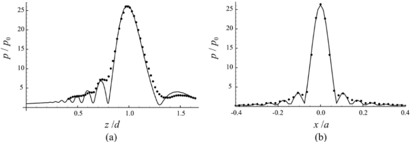
The validation of the developed numerical code was first carried out for the case of a focused circular trans-ducer. The results of comparison of measured and simu-lated acoustic fields are presented in Figs. 1 and 2. Fig. 1 exemplifies the case of small-amplitude (linear) excita-tion. The sound source used in the experiment is a custom transducer with the piezoelectric ceramic from meggitt
(Kvistgaard, denmark). The radius of the transducer is
a = 23.5 mm and the focal length is d = 48.6 mm. a
10-cycle Gaussian pulse, centered at 1 mHz, was gener-ated using matlab (The mathWorks Inc., natick, ma) and then transmitted through a GpIb port (national In-struments corp., austin, TX) to an arbitrary function generator (33220a, agilent Technologies Inc., palo alto, ca). The signal was then amplified using a power ampli-fier (150a100b, ampliampli-fier research, souderton, pa) and transmitted to the transducer mounted in a water bath. The on-source pressure amplitude p0 was estimated by fitting the measured axial pressure profile with that cal-culated by means of Field II, software that is considered a standard in the modeling of linear wave propagation [36]. as a result, p0 was found to be 5 kpa. The transmitted sig-nals were measured at different distances in the ultrasonic field using a calibrated needle hydrophone (0.075 mm, precision acoustics ltd., dorchester, UK) mounted on a XyZ positioning system (Trioptics GmbH, Wedel, Ger-many). The received signals were displayed on a digital oscilloscope (Tektronix, beaverton, or) and transferred to a personal computer through a GpIb port. The axial pressure profile was measured with the spatial step size 1 mm ± 0.005 mm, and the lateral pressure profile was measured with the spatial step size 0.5 mm ± 0.005 mm. The accuracy of measurement of signal amplitudes was 13%. This value corresponds to the hydrophone calibra-tion error specified in the manufacturer’s datasheet.
The parameters used in the simulations were: c = 1480 m/s, δ = 4.5 × 10⁻⁶ m2/s, ρ = 1000 kg/m3, and β = 3.5. These values correspond to water. Fig. 1(a) shows the measured (circles) and the simulated (solid line) axial pressure profiles. Fig. 1(b) shows the measured and the simulated lateral pressure profiles in the focal plane. The axial distance z is normalized by the focal length d, and the lateral distance x is normalized by the transducer ra-dius a. The pressure is normalized by the on-source pres-sure amplitude p0. The computational domain spanned an area with −53.7 mm ≤ x, y ≤ 53.7 mm and 0 ≤ z ≤
zmax = 77.8 mm. The simulation was performed with the following discretization steps: ∆t = 0.01/f = 10−8 s, ∆x = ∆y = 0.2λ = 0.296 mm, and ∆z = 0.1λ = 0.148 mm, where f is the driving frequency and λ = c/f is the sound wavelength. as reported in studies on the numerical in-tegration of the Westervelt equation (see, for example, [24] and [30]), the maximum size of the temporal step is usually estimated by the nyquist rate: ∆t = 1/(2fmax), where fmax is the frequency of the highest harmonic to be tracked. The size of the spatial steps is usually set to be 10 to 20 steps per wavelength. In each specific case, however, p r t p r d F t d c r d r d r ( , )= +( ) +
(
+( ) −)
tan ≤ > 0 2 2 1 1 1 0 / / for for α dd tan α (8)the choice of the step sizes is determined by the specific conditions of a simulated situation and is based on the tradeoff between accuracy and computational effort. We used the same approach, i.e., the choice of the aforemen-tioned step sizes was based on an attempt to get satisfac-tory agreement with experiments at a minimal possible computation time. The same rule was used when choosing the discretization step sizes in simulations described later. The number of time steps was set to be equal to Nts = (Tpro + Tsig + Tdel)/∆t, where Tpro is the time during which sound propagates from z = 0 to zmax, Tsig is the du-ration of the driving signal, and Tdel is the delay between the signals that are emitted from the center of the trans-ducer and from the edge of the transtrans-ducer. as one can see in Fig. 1, the simulated curves and the experimental data are in good agreement and the main characteristics of the measured pressure profiles are well predicted by the numerical results. To quantify the difference between the experimental measurements and the simulations, we cal-culated the l2 norm error [24], which is defined as
ε =
∑
−∑
( ) ( ) , exp exp p p p i i i i i sim 2 2 (10)where piexp and p
isim are experimental and simulated val-ues, respectively. For the curves in Figs. 1(a) and 1(b), the l2 norm errors were found to be ε = 0.14 and 0.06, respec-tively. It should be noted that the experimental data in Fig. 1(a) do not demonstrate minima in the prefocal re-gion which are present on the simulated curve. This is explained by the influence of noise, which was substantial because a weak signal was used to get the regime of linear wave propagation.
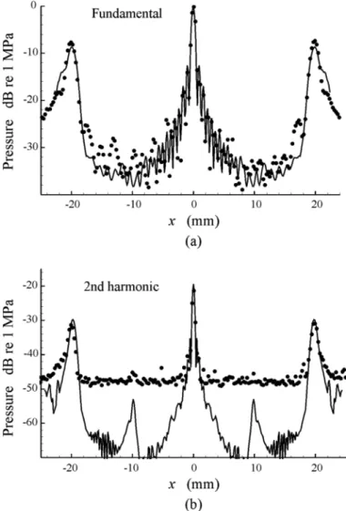
The case of finite-amplitude (nonlinear) excitation is exemplified in Fig. 2. The sound source is a piezoelectric transducer (sofranel, sartrouville, France) with radius a = 13.4 mm and focal length d = 57 mm. The experimen-tal procedure was similar to that described previously. The center frequency and the on-source pressure ampli-tude were set to be 2.25 mHz and 54 kpa, respectively. To estimate the value of the on-source pressure amplitude, the measured signal was filtered at the fundamental fre-quency and then the axial pressure profile of this filtered signal was fitted with that calculated by Field II [36]. Field II is known to be a program for the modeling of linear wave propagation. Therefore, it should be empha-sized that its use in the aforementioned operation is pos-sible because it is applied to the linearized signal involving the fundamental component alone. The data presented in Fig. 2 show the axial pressure profiles for the fundamental and the second-harmonic components. The simulation was performed in an area with −27.6 mm ≤ x, y ≤ 27.6 mm and 0 ≤ z ≤ 85.5 mm. The discretization steps were set to ∆t = 0.01/f = 0.44444 × 10⁻⁸ s, ∆x = ∆y = 0.2λ = 0.13156 mm, and ∆z = 0.04λ = 0.02631 mm. The number of time steps Nts was calculated by the same equation as used in Fig. 1. The experimental and theoretical curves for the fundamental component were obtained by filtering in the range from 1.5 to 3 mHz (matlab, butterworth filter, order 3). similarly, the second harmonic was extracted using a band-pass filter in the range from 3.5 to 5.5 mHz. Fig. 1. a comparison of the simulated (solid lines) and measured (circles) pressure profiles for a circular focused transducer (a = 23.5 mm, d = 48.6 mm) at a center frequency of 1 mHz and the on-source pressure amplitude p0 = 5 kpa: (a) axial profile and (b) lateral profile in the focal plane.
Fig. 2. a comparison of the simulated (solid lines) and measured (circles) axial profiles for the fundamental and the second-harmonic components. The sound source is a circular focused transducer (a = 13.4 mm, d = 57 mm) excited at 2.25 mHz and p0 = 54 kpa.
as one can see, the behavior of the second harmonic of the pressure filed is well predicted by the numerical cal-culation. The l2 norm errors for the fundamental and the second harmonic are ε = 0.08 and 0.12, respectively. It should be noted that the simulation of the nonlinear case requires a smaller step size in the z direction. To repre-sent the second harmonic correctly, the step size should provide about 10 samples per spatial wavelength that cor-responds to the second harmonic frequency. This observa-tion agrees with the comment made in [30], namely that the fine discretization is the main issue of finite-difference methods, which necessitates a great computational effort in such cases as the simulation of the three-dimensional nonlinear wave propagation. discussion of this problem as applied to the KZK equation can be found in [37].
B. Phased-Array Transducer
comparisons of experimental and numerical results ob-tained for a phased array transducer are presented in Figs. 3–6. The experiments were performed using a 128-element pZT linear-array probe (Vermon, Tours, France) with a pitch of 305 µm and an elevation of 7.12 mm. The probe was centered at 4 mHz, with a fractional bandwidth of 60% at −3 db. In our experiments, however, the probe was not excited at its center frequency. as an excitation signal, a 20-cycle Gaussian pulse with a center frequency of 2.5 mHz was used. This frequency was chosen so that both the fundamental and second harmonic fall within the passband of the transducer. The pulse was generated using matlab and then transmitted to a 128-channel fully pro-grammable ultrasound system (Wavemaster, m2m, les Ulis, France) equipped with analog transmitters. To verify theoretical predictions, the probe was adapted to gener-ate grating lobes. Hence, only 1 of 4 elements was driv-en, so the probe functioned as a 32-element linear,array transducer. The transmit focal law was calculated by the
program package cIVa (cEa, Gif-sur-yvette, France) to obtain a focal length of 40 mm. The propagating signals received from the hydrophone were displayed on a digi-tal oscilloscope and then transferred to matlab for post-processing (signal filtering). during every measurement, to decrease the noise level, 16 consecutive signals were averaged. The axial pressure profiles were measured with the spatial step size 0.5 mm ± 0.005 mm, and the lateral pressure profiles were measured with the spatial step size 0.25 mm ± 0.005 mm.
Figs. 3–5 illustrate the case of a zero steering angle, where the sound beam propagates along the central axis of the transducer. The computation domain had the fol-lowing limits: −39 mm ≤ x ≤ 39 mm, −6 mm ≤ y ≤ 6 mm, and 0 mm ≤ z ≤ 60.3 mm. The discretization steps were set to ∆t = 0.01/f = 0.4 × 10⁻⁸ s, ∆x = 0.23λ = 0.13616 mm, ∆y = 0.25λ = 0.148 mm, and ∆z = 0.05λ = 0.0296 mm. The number of time steps was calculated as Nts = (Tpro + Tsig + ∆tmax)/∆t, where ∆tmax is the maximum focusing delay given by (9). Fig. 3 shows the axial pressure profiles for the fundamental and the sec-Fig. 3. case of a 32-element array transducer. a comparison of the
simu-lated (solid lines) and measured (circles) axial profiles for the fundamen-tal and the second-harmonic components. The focal length is 40 mm and the steering angle is 0°. The excitation is a 20-cycle Gaussian pulse with a center frequency of 2.5 mHz. The simulated curves were obtained at the on-source pressure amplitude 340 kpa and the pitch 1262 µm.
Fig. 4. lateral profile in the focal plane for the same case as in Fig. 3: (a) fundamental component and (b) second-harmonic component. The solid lines show the simulated curves and the circles indicate the experimental measurements.
ond-harmonic components, which were obtained using a band-pass filter (matlab, butterworth filter, order 3) in the ranges from 1.75 to 3.25 mHz and from 4 to 6 mHz, respectively. The l2 norm errors for the fundamental and the second harmonic are ε = 0.09 and 0.2, respectively. Fig. 4 shows the lateral pressure profiles in the focal plane for the fundamental and the second-harmonic components for the same case as in Fig. 3. The l2 norm error for the data in Fig. 4(a) is 0.15. The presence of strong noise in Fig. 4(b) interferes with an adequate evaluation of the l2 norm error. The side peaks in Fig. 4 are grating lobes. The value of the pitch was intentionally set to be large enough to check whether the developed code is capable of capturing the grating lobe generation. In the case un-der consiun-deration, the location of the grating lobes is ex-pected, according to the equation of grating lobes [38], to be at about 28° (21 mm) from the central propagation axis. note that the grating lobes are located far outside the 16° validity region of the KZK equation. In Fig. 5, the measured and simulated waveforms at the focal point and spectra corresponding to these waveforms are pre-sented. as one can see, Figs. 3–5 demonstrate satisfactory agreement between the experimental and numerical
re-sults. The position and the form of the main lobe and the grating lobes are well predicted for both the fundamental and the second-harmonic components. There is a differ-ence in the peak amplitude of the second harmonic. This disagreement is especially visible in Fig. 3. one possible explanation is as follows. Fig. 4(b) reveals that the central peak of the second harmonic is very narrow in the lateral direction, and hence even a very small deviation from the central axis in the process of measurement can result in understating the peak amplitude. such a deviation can be caused by accumulating errors in the experimental spa-tial step size as the lateral distance is measured from the maximum negative value of x.
Fig. 6 shows the measured and simulated lateral pres-sure profiles in the case in which the steering angle is 20°. The dimensions of the computation domain were −48.7 mm ≤ x ≤ 48.7 mm, −6 mm ≤ x ≤ 6 mm, and 0 mm ≤ x ≤ 40.5 mm. The discretization steps were set to ∆t = 0.01/f = 0.4 × 10⁻⁸ s, ∆x = 0.23λ = 0.13616 mm, ∆y = 0.25λ = 0.148 mm, and ∆z = 0.06λ = 0.03552 mm. Fig. 5. (a) simulated and measured waveforms at the focal point for the
case shown in Fig. 3. (b) spectra corresponding to the waveforms shown in Fig. 5(a). The solid lines show the simulated curves and the circles indicate the experimental measurements.
Fig. 6. case of a 32-element array transducer. a comparison of the simu-lated (solid lines) and measured (circles) lateral profiles at the steering angle equal to 20°: (a) fundamental component and (b) second-harmonic component. The on-source pressure amplitude is 400 kpa. The other pa-rameters are as in Fig. 3. The profiles were obtained at a distance from the transducer equal to the focal length (40 mm).
The number of time steps was determined in the same way as in the case of zero steering angle. The pressure profiles were obtained at a distance from the transducer equal to the focal length (40 mm). In this case, the posi-tion of the main lobe is expected to be at about 14.5 mm (20°) to the left of the central axis. The first-order grat-ing lobe is expected, accordgrat-ing to the equation of gratgrat-ing lobes [38], to be at about 5 mm (7.3°) to the right of the central axis, and the second-order grating lobe, at about 29.7 mm (36.6°). Thus, the second-order grating lobe is located far beyond the validity region of the KZK equa-tion. Fig. 6 shows a satisfactory fit of the simulated curves to the experimental data for both the fundamental and the second harmonic. The l2 norm error for the data in Fig. 6(a) is 0.3.
The characteristic computational time in the cases shown in Figs. 3–6 is 7 to 9 h. The calculations were per-formed on a personal computer Hp compaq 6200 pro mT pc (Hewlett-packard co., palo alto, ca) with a 2.90-GHz Intel pentium G850 cpU (Intel corp., santa clara, ca) and 4 Gb of ram.
IV. conclusions
a numerical code has been developed to model acous-tic fields generated by ultrasound transducers. The code is based on a 3-dimensional numerical solution of the full Westervelt equation. The numerical scheme was realized by using the explicit finite-difference time-domain (FdTd) method. The main purpose of the work was to verify, by comparing numerical and experimental results, the abil-ity of the Westervelt equation to predict the behavior of nonlinear ultrasound beams generated by phased-array transducers. simulations and experimental measurements were carried out for cases that were not investigated in the preceding works in which similar numerical approaches were used. In particular, the developed code was applied to simulating the generation of grating lobes at zero and nonzero steering angles in cases in which the grating lobes are located far beyond the validity region of the KZK equation.
The initial validation of the developed numerical code was carried out by using experimental data obtained for two focused circular transducers having different diam-eters and focal lengths. The first transducer, driven at a center frequency of 1 mHz, was used to measure the axial and lateral pressure profiles in the case of small-amplitude excitation. The second transducer, driven at 2.25 mHz, was used in the regime of finite-amplitude excitation to measure the axial pressure profiles for the fundamental and the second-harmonic components. In both linear and nonlinear cases, good agreement between the measured and the simulated data was demonstrated.
Experimental measurements were then carried out for a modified 32-element linear-array transducer. The speci-fications of the transducer were modified so as to generate grating lobes. pressure profiles for the fundamental and
the second-harmonic components were measured at 0° and 20° steering angles. The conditions of wave propagation were set in such a way that the grating lobes were gener-ated far beyond the validity region of the KZK equation. comparison of the experimental and numerical results has shown that they are in satisfactory agreement for both the fundamental and the second-harmonic components in all the cases tested.
The results of the present work confirm that a 3-d FdTd implementation of the Westervelt equation is ca-pable of providing adequate simulation of nonlinear ultra-sound fields generated by phased-array transducers. This approach allows one to predict with satisfactory accuracy nonlinear wave propagation even in relatively complicated situations, namely when the propagation of an ultrasonic beam at a nonzero steering angle is accompanied by the generation of grating lobes which are located at large an-gles from the central propagation axis. The shortcoming of the presented approach is that it requires quite a small step size along the main propagation axis (z-axis) to catch higher harmonics correctly; the step size decreases with increasing excitation frequency. as a result, the simula-tion of 3-d nonlinear wave propagasimula-tion can be very time consuming at high frequencies. solving this problem could be the objective of further work.
references
[1] E. a. Zabolotskaya and r. V. Khokhlov, “quasi-plane waves in the nonlinear acoustics of confined beams,” Sov. Phys. Acoust, vol. 15, no. 1, pp. 35–40, 1969.
[2] V. p. Kuznetsov, “Equation of nonlinear acoustics,” Sov. Phys.
Acoust, vol. 16, no. 4, pp. 467–470, 1970.
[3] m. F. Hamilton and c. l. morfey, “model equations,” in Nonlinear
Acoustics, san diego, ca: academic press, 1998, pp. 41–63.
[4] J. naze Tjøtta, s. Tjøtta, and E. H. Vefring, “propagation and interaction of two collimated finite amplitude sound beams,” J.
Acoust. Soc. Am., vol. 88, no. 6, pp. 2859–2870, 1990.
[5] J. naze Tjøtta, s. Tjøtta, and E. H. Vefring, “Effects of focusing on the nonlinear interaction between two collinear finite amplitude sound beams,” J. Acoust. Soc. Am., vol. 89, no. 3, pp. 1017–1027, 1991.
[6] a. c. baker, “nonlinear pressure fields due to focused circular aper-tures,” J. Acoust. Soc. Am., vol. 91, no. 2, pp. 713–717, 1992. [7] a. c. baker and V. F. Humphrey, “distortion and high-frequency
generation due to nonlinear propagation of short ultrasonic pulses from a plane circular piston,” J. Acoust. Soc. Am., vol. 92, no. 3, pp. 1699–1705, 1992.
[8] y.-s. lee and m. F. Hamilton, “Time-domain modeling of pulsed finite-amplitude sound beams,” J. Acoust. Soc. Am., vol. 97, no. 2, pp. 906–917, 1995.
[9] m. a. averkiou and m. F. Hamilton, “measurements of harmonic generation in a focused finite-amplitude sound beam,” J. Acoust.
Soc. Am., vol. 98, no. 6, pp. 3439–3442, 1995.
[10] r. o. cleveland, m. F. Hamilton, and d. T. blackstock, “Time-domain modeling of finite-amplitude sound in relaxing fluids,” J.
Acoust. Soc. Am., vol. 99, no. 6, pp. 3312–3318, 1996.
[11] m. a. averkiou and m. F. Hamilton, “nonlinear distortion of short pulses radiated by plane and focused circular pistons,” J. Acoust.
Soc. Am., vol. 102, no. 5, pp. 2539–2548, 1997.
[12] m. d. cahill and a. c. baker, “numerical simulation of the acoustic field of a phased-array medical ultrasound scanner,” J. Acoust. Soc.
Am., vol. 104, no. 3, pp. 1274–1283, 1998.
[13] a. bouakaz, c. T. lancée, p. Frinking, and n. de Jong, “simula-tions and measurements of nonlinear pressure field generated by linear array transducers,” in Proc. 1999 IEEE Ultrasonics Symp., 1999, pp. 1511–1514.
draulic lithotripter with the KZK equation,” J. Acoust. Soc. Am., vol. 106, no. 1, pp. 102–112, 1999.
[15] r. J. Zemp, J. Tavakkoli, and r. s. c. cobbold, “modeling of non-linear ultrasound propagation in tissue from array transducers,” J.
Acoust. Soc. Am., vol. 113, no. 1, pp. 139–152, 2003.
[16] X. yang and r. o. cleveland, “Time domain simulation of nonlinear acoustic beams generated by rectangular pistons with application to harmonic imaging,” J. Acoust. Soc. Am., vol. 117, no. 1, pp. 113–123, 2005.
[17] p. d. Fox, a. bouakaz, and F. Tranquart, “computation of steered nonlinear fields using offset KZK axes,” in Proc. 2005 IEEE
Ultra-sonics Symp., 2005, pp. 1984–1987.
[18] V. a. Khokhlova, a. E. ponomarev, m. a. averkiou, and l. a. crum, “nonlinear pulsed ultrasound beams radiated by rectangular focused diagnostic transducers,” Acoust. Phys., vol. 52, no. 4, pp. 481–489, 2006.
[19] J. E. soneson, “a parametric study of error in the parabolic ap-proximation of focused axisymmetric ultrasound beams,” J. Acoust.
Soc. Am., vol. 131, no. 6, pp. El481–El486, 2012.
[20] T. Kamakura, T. Ishiwata, and K. matsuda, “model equation for strongly focused finite-amplitude sound beams,” J. Acoust. Soc.
Am., vol. 107, no. 6, pp. 3035–3046, 2000.
[21] p. Westervelt, “parametric acoustic array,” J. Acoust. Soc. Am., vol. 35, no. 4, pp. 535–537, 1965.
[22] I. m. Hallaj and r. o. cleveland, “FdTd simulation of finite-am-plitude pressure and temperature fields for biomedical ultrasound,”
J. Acoust. Soc. Am., vol. 105, no. 5, pp. l7–l12, 1999.
[23] d. botteldooren, “acoustical finite-difference time-domain simula-tion in a quasi-cartesian grid,” J. Acoust. Soc. Am., vol. 95, no. 5, pp. 2313–2319, 1994.
[24] y. Jing, m. Tao, and G. T. clement, “Evaluation of a wave-vec-tor-frequency-domain method for nonlinear wave propagation,” J.
Acoust. Soc. Am., vol. 129, no. 1, pp. 32–46, 2011.
[25] a. Karamalis, W. Wein, and n. navab, “Fast ultrasound image sim-ulation using the Westervelt equation,” in Medical Image Computing
and Computer Assisted Intervention–MICCAI, 2010, pp. 243–250.
[26] J. Huang, r. G. Holt, r. o. cleveland, and r. a. roy, “Experimen-tal validation of a tractable numerical model for focused ultrasound heating in flow-through tissue phantoms,” J. Acoust. Soc. Am., vol. 116, no. 4, pp. 2451–2458, 2004.
[27] r. d. purrington and G. V. norton, “a numerical comparison of the Westervelt equation with viscous attenuation and a causal propaga-tion operator,” Math. Comput. Simul., vol. 82, no. 7, pp. 1287–1297, 2012.
[28] c. W. connor and K. Hynynen, “bio-acoustic thermal lensing and nonlinear propagation in focused ultrasound surgery using large fo-cal spots: a parametric study,” Phys. Med. Biol., vol. 47, no. 11, pp. 1911–1928, 2002.
[29] G. F. pinton, J. dahl, s. rosenzweig, and G. E. Trahey, “a het-erogeneous nonlinear attenuating full-wave model of ultrasound,”
IEEE Trans. Ultrason. Ferroelectr. Freq. Control, vol. 56, no. 3, pp.
474–488, 2009.
[30] J. Huijssen and m. d. Verweij, “an iterative method for the com-putation of nonlinear, wide-angle, pulsed acoustic fields of medical diagnostic transducers,” J. Acoust. Soc. Am., vol. 127, no. 1, pp. 33–44, 2010.
[31] I. m. Hallaj, r. o. cleveland, and K. Hynynen, “simulations of the thermo-acoustic lens effect during focused ultrasound surgery,” J.
Acoust. Soc. Am., vol. 109, no. 5, pp. 2245–2253, 2001.
[32] J. H. mathews and K. d. Fink, Numerical Methods, Upper saddle river, nJ: prentice Hall, 1999, ch. 6.
[33] G. cohen and p. Joly, “construction and analysis of fourth-order finite difference schemes for the acoustic wave equation in nonho-mogeneous media,” SIAM J. Numer. Anal., vol. 33, no. 4, pp. 1266– 1302, 1996.
[34] m. F. Hamilton, “comparison of three transient solutions for the axial pressure in a focused sound beam,” J. Acoust. Soc. Am., vol. 92, no. 1, pp. 527–532, 1992.
[35] l. azar, y. shi, and s.-c. Wooh, “beam focusing behavior of linear phased arrays,” NDT Int., vol. 33, no. 3, pp. 189–198, 2000. [36] J. a. Jensen, “Field: a program for simulating ultrasound systems,”
Med. Biol. Eng. Comput., vol. 34, suppl. 1, pt. 1, pp. 351–353, 1996.
“Fast simulation of second harmonic ultrasound fields,” in Proc.
2009 IEEE Int. Ultrasonics Symp., 2009, pp. 2394–2397.
[38] b. d. steinberg, Principles of Aperture and Array System Design. new york, ny: Wiley, 1976.
Alexander A. Doinikov received his ph.d. degree in theoretical
phys-ics in 1990 from the belarus state University, minsk, belorussia. From 1989 to 1991, he worked as a junior researcher at the Institute of applied physics problems of the belarus state University. From 1991 to 1993, he was a senior researcher in the department of applied mathematics of the same university. From 1993 to 1998, he worked as a senior researcher at the research Institute for nuclear problems of the belarus state Uni-versity, and since 1998, he has been a principal researcher at the same institute. In February 2009, he joined the research unit InsErm U930 at the Université François rabelais de Tours, France, where he currently works as an invited scientist. His current research interests include physi-cal acoustics and mediphysi-cal ultrasonics.
Anthony Novell received his m.sc. degree in
medical imaging technologies in 2007 and his ph.d. degree in 2011 from the University François rabelais, Tours, France. He pursued postdoctoral research at the French Institute for Health and medical research (Inserm) in Tours, France, un-der the guidance of dr. ayache bouakaz. He joined the dayton lab at the University of north carolina, chapel Hill, nc, in 2014, with the aid of a postdoctoral research Fellowship from the French arc Foundation. His research mainly fo-cuses on contrast agent imaging, capacitive micromachined ultrasonic transducers (cmUTs), and therapeutic ultrasound.
Pierre Calmon received his ph.d. degree in
physics in 1990 from the University of paris sud, France. He then joined the Ultrasonic ndE (non-destructive evaluation) laboratory of the cEa (French atomic Energy commission) and worked on ultrasonic modeling. His activities focused on the development of semi-analytical approaches for the simulation of ultrasonic inspections and array imaging. From 2000 to 2005, he was involved in the development of the cIVa ndE simulation platform and coordinated software developments. over the same period, he was the head of the simulation and processing Ultrasonic laboratory of cEa. since 2008, he has coordinated ndE core research at cEa as research director.
Ayache Bouakaz graduated from the University
of sétif, algeria, from the department of Electri-cal Engineering. He obtained his ph.d. degree in 1996 from the department of Electrical Engineer-ing at the Institut national des sciences appli-quées de lyon (Insa lyon), France. In 1998, he joined the department of bioengineering at The pennsylvania state University in state college, pa, where he worked as a postdoc for 1 year. From February 1999 to november 2004, he was employed at the Erasmus University medical cen-ter, rotterdam, The netherlands. His research focused on imaging, ul-trasound contrast agents, and transducer design. since January 2005, he has held a permanent position as a director of research at the French Institute for Health and medical research, InsErm, in Tours, France, where he heads the ultrasound and imaging laboratory. His research fo-cuses on imaging and therapeutic applications of ultrasound and micro-bubbles.