Explaining Trade Flows: Traditional and New Determinants of Trade Patterns

HAL Id: halshs-00557125

https://halshs.archives-ouvertes.fr/halshs-00557125

Preprint submitted on 18 Jan 2011

HAL is a multi-disciplinary open access archive for the deposit and dissemination of sci-entific research documents, whether they are pub-lished or not. The documents may come from

L’archive ouverte pluridisciplinaire HAL, est destinée au dépôt et à la diffusion de documents scientifiques de niveau recherche, publiés ou non, émanant des établissements d’enseignement et de

To cite this version:

Julien Gourdon. Explaining Trade Flows: Traditional and New Determinants of Trade Patterns. 2011. �halshs-00557125�

Document de travail de la série

Etudes et Documents

E 2007.06

EXPLAINING TRADE FLOWS: TRADITIONAL AND NEW DETERMINANTS OF TRADE PATTERNS

Julien GOURDON

CERDI - UMR CNRS 6587 - Université Clermont 1

mai 2007

Abstract

An empirical tradition in international trade seeks to establish whether the predictions of factor abundance theory match with the data. The relation between factor endowments and trade in goods (commodity version of Hecksher-Ohlin) provide mildly encouraging empirical results. But in the analysis of factor service trade and factor endowments (factor content version of HO), the results show that it performs poorly and reject strict HOV models in favor of modifications that allow for technology differences, consumer’s preferences differences, increasing returns to scale or cost of trade. In this paper we test if these “new” determinants help us to improve our estimation of trade patterns in commodities. Since the commodity version allows obtaining a large panel data we also compare two periods, pre and post 1980. We use a Heckman procedure to allow for non linearity in the relation between factors endowments and net exports and between trade intensity and net exports. The results show that adding the “new” determinants of factor content studies help us to improve the prediction of being specialized in the different manufactured products. However specialization according to factor endowments is stronger than ever, especially concerning the specialization according to human capital endowment. Trade patterns are also determined by trade intensity. Here differences in technology, trade policy, transport and transaction costs, explain the difference in trade intensity.

JEL Classification: F11, F14, F2

1. Introduction

In the neo classical general equilibrium model of international trade, countries trade with each other because of their differences. The Hecksher-Ohlin model holds on the idea that trade patterns depend on the relative differences in the factor endowment of countries. Empirical studies have often shown a weak link between factor endowment and trade flows, both within countries (between regions) and between countries. Those studies tested the two versions of the HO model1_{. In the}

commodity version, a capital abundant country will export a capital intensive goods and the generalization in a factor version (Vanek, 1968). In that version, a capital abundant country will export capital services. Many improvements have been tested concerning the factor content version2_{, but their implications concerning net trade in commodities}

seems relatively weak. Predicting net trade in commodities in an nxn world is not straightforward, notably because input-output linkages preclude a linear relation between factor endowment and net exports. Furthermore, unlike in the Ricardian model, we cannot obtain a ladder of comparative advantage3_{. This paper is a contribution to the study of}

pattern of trade for developing countries.

So far, starting with Leamer (1984) has shown that trade specialization for primary goods is highly dependent on the differences in endowments of natural resources, whereas the result for manufactured

1

See Annex II

2

There are also improvements concerning the literature about specialization in production: some authors (ex: Harrigan 1997) argue that’s more important to look at the pattern of specialization rather than the pattern of trade since economists won’t be able to understand trade until they understand specialization.

3

Furthermore, because we will also studying the effect of trade on income distribution studied it is necessary.

goods is not clear (even though this does not appear in his book, he developed the idea at a later date, notably in an article written in collaboration with Bowen and Sveikauskas (1987)). Subsequent attempts also encountered little success with regard to manufactured goods, the coefficients either being non-significant or carrying the wrong sign. Nevertheless, some studies (e.g. Minford (1989), Balassa and Bauwens (1988)), find that North-South trade can be explained by difference in skill endowments (but not in capital endowments).

The HOV theorem has frequently been rejected in favor of statistical hypotheses such as a zero correlation between factors’ endowments and trade patterns. Facing those unclear results, the widespread view in the middle of 90’s could be resumed by Leamer and Levinsohn appraisal (1995) of the empirical performance of factors endowment theories: “It is more convenient to estimate the speed of arbitrage rather than test if the arbitrage is perfect and instantaneous”. Moreover, as Trefler said (1995), there is no general equilibrium model of factor service trade that is known to perform better than the HOV theorem.

Then in the middle of the 90’s an expanding literature on the determinant of trade patterns used differences in consumers’ preferences, in technology or in returns to scale to explain trade patterns. Differences in technology (suggested by Ricardo) have been frequently used (Trefler 1995, Davis and Weinstein 2001) and, not surprisingly, have considerably improved the prediction of trade in factor services. Difference in consumer’s preferences could relate to home bias consumption (Trefler 1995) or non homothetic preferences due to differences in income per capita (Markusen 1986 or Jones and al. 1999). Finally increasing returns to scale in some sectors is also useful to explain some factor service trade flows (Antweiler and Trefler 2002, Head and Ries 2001).

All these “new” determinants have been used in factor content studies, which have been applied mostly to developed countries because only these countries have data allowing to compute the factor content of trade in each sector in an economy. In addition to factor endowments, these studies use “new” determinants to explain why a country is a net exporter of one factor and to explain the excess of factor content in exports relatively to factor supply. Some use also these “new” determinants to explain the specialization in production (Harrigan 1997, Schott 2003).

To learn more about the determinants of comparative advantage one needs to include many countries and, if possible over a long enough period of time, to see if this determinants have changed through time. In the absence of reliable input-output data needed to compute the net factor content of trade, one way to proceed is to study the determinants of net trade on commodities (i.e. to rely on the commodity version of the HOV theorem). Lederman and Xu (2001) include these “new” determinants in a commodity version for a panel of 57 countries over 25 years for 10 products groups clusters introduced by Leamer (1984). They used a probit estimation to test the impact of factors endowments on net exports which is a better way to control for non linearity than the way used in previous studies on commodities (Leamer 1984 and 1987).

This paper extends this commodity version analysis in the following ways. First we include differences in consumers’ preferences and differences in returns to scale as a determinant of comparative advantage and not only as determinants for trade intensity. Second we use total factor productivity as a measure for differences in technology, rather than expenditure in research and development. Third, our sample of 71 countries over 40 years allows us to discern two periods: pre-1980 and post-1980, and to isolate any changes in the relative importance of conventional

and new factors during the period under review. Fourth we use International Trade Center (ITC) and National Asia Pacific Economic and Scientific (NAPES) commodities classification rather than Leamer’s classification. This allows us to obtain better results on manufactured commodities4_{. Finally rather than use “unadjusted” factor endowments}

measures, we use a measure of relative factor endowment (relative to the world endowment) as in Spilimbergo and al. (1999) in order to be closer to the theory. Also we distinguish three sorts of skills.

To anticipate, our results show that HOV is “alive and well” and furthermore that the “new” determinants have not more explanatory power in the period 1980-2000 compared with the period 1960-1980. Nonetheless adding the new determinants of factor content studies help us to improve the prediction of being specialized in different manufactured products. This result was already found by previous studies. That factor endowment matter is especially robust concerning specialization according to human capital endowment. This result is probably attributable to our distinguishing among three sorts of skills. Trade patterns are also determined by trade intensity, here difference in technology, trade policy, transport and transaction costs explain the difference in trade intensity. More generally, the results in this chapter provide a further justification for our concentration in the next chapter on factor endowments as factors contributing to explain why trade have different effects on income inequality.

The paper is organized as follows. Section 2 reviews the presentation of the HO model and the amendments added in the factor content studies. Section 3 describes the empirical approach, the data used and their organization between explanatory variables for comparative

4

advantage and for trade intensity as well as the cluster’s construction. Section 4 presents the econometric results and section 5 concludes.

2. Approaches to explain trade patterns

This section presents the framework and justifies the empirical approach. Consider the standard Hecksher-Ohlin theory, with a world of C

countries

(

c

=

1,....,

C

)

,I industries

(

i

=

1,....,

I

)

and F factors

(

f

=

1,....,

F

)

. LetYc (I×1) the output in country

c

. The factor content of YcisAYc, whereAis a matrix (F×I ) of factor content coefficient. Let c

V the factor endowment of country

c

, the full employment implies thatAYc =Vc. For the world we get:AYw=Vw, assuming that factor intensity (technology)

Ais identical in each country for each good and the assumption that the technology is identical assumes that the factor price equalization holds in equilibrium.

If we assume that each country consumes the product in the same proportion (identical homothetic preferences) we have: c c w

C =s Y where

c

s is the country’s consumption share: sc = pCc pCw where p is the vector of internal prices. Under balanced trade, the vector of net exportsTc

is the difference between production and consumption

(

)

1

c c c c c w

T =Y −C =A− V −s V (1.1)

The link between factor prices and commodity prices is implied by the zero profit conditions, where

w

is the vector of factor returns:Aw= p. Here equation 1.1 says that trade in each industry is linearly related to factor endowments.

In higher dimensions it becomes impossible to state the HO theorem in a useful way analogous to its statement in the 2 –dimensional case. What

remains true in higher dimensions is that the inverse of a strictly positive matrix has at least one positive and at least one negative element in every row and column (Either 1974). So each factor has at least one friend and at least one enemy among goods. But we have to assume here thatA is invertible (it is square withI =F ). That is why Vanek rephrased the HO theorem in a correct way, which is called the factor content version (in contrast to the commodity version). A country with balanced trade will export the services of abundant factors and import the services of scarce factors. This equation does not depend on any assumptions about the dimension or invertibility of the matrixA.

(

)

c c c c w

F =AT = V −s V (1.2)

2.1 Empirical approach to “test” the theorem

The three main approaches used to assess the HO theorem are presented in table 1. Column 2 describes the basic approach, column 3 extensions to that approach, column 4 the estimation technique and column 5 the results.

The first (Table 1a), uses the factor content version (equation 1.2) and directly link net trade in factor services and factor endowments. In order to do that, authors use an input-output matrix by sector to measure the factor intensity in each sector5 _{and then, knowing the net exports of}

each sector, they can calculate the net exports of factors.

(

)

c c c c w

F = AT = V −s V (1.2)

This approach is undeniably the most appropriate technique to test the HOV proposition, since all parameters are measured, none are estimated econometrically. However it requires data that are not available for a large

5

number of countries and for many years (as input-output data). Therefore those analyses have only appeared relatively recently and are always imperfect. They often cover just one year (Bowen and al., 1987, Trefler, 1995, Davis and Weinstein, 2001, Schott, 2003), or do not use real input output matrix from all countries6 _{(Bowen and al. 1987, Trefler 1995,}

Estervadeordal and Taylor 2002), or do not account for natural resources (Davis and Weinstein). These misspecifications (e.g. imposing the same input-output matrix for all countries) lead some authors like Estervadeordal and Taylor (2002) to “give HO a break”; that is, to argue that one should stop the test on factor content until reliable and sufficient data becomes available for a large panel of countries for a long time period. However those studies provide interesting improvements that are useful for other forms of the HO test. Notably, they have relaxed some central assumptions from the HO model (similarity in technology and consumer preferences, constant returns to scale and no trade impediments) to obtain “new” determinants. These so called “new” determinants improve the explanation of trade patterns. Not surprisingly, generally, they find that a strict HO model (just considering difference in factor endowments) performs poorly.

6

Table 1a: Studies of factor content in trade

Authors/Sample Factors Extensions Empirical Technique Results

Bowen, Leamer Sveikauskas 1987 27 countries in 1967 K, 3 sorts of land, 7 sorts of labor Technological difference in using US I-O matrix Non proportional consumption

Proportion of factors for which the sign of net trade in factor matched the sign of the corresponding supply in factor

Sign test7: no supportive, the role of technological is not clear. Trefler 1995 33 countries in 1983 K, 2 sorts of land, 7 sorts of labor Technological difference in using US I-O matrix Home bias in consumption

Compare for nine factors the difference in endowment to the net trade (factor content test). Then add neutral technology difference and Armington home bias in consumption

Sign test and variance ratio test8: supportive if we allow for neutral technological difference and home bias in consumption Davis and Weinstein 2001 10 countries and the ROW (20 countries aggregated) in 1985

K and Labor Technological difference in using I-O matrix for all 10 countries Trade impediments Non homothetic preferences

Estimate with identical technology (US), then with Hicks neutral difference and no Hicks neutral difference. And finally with trade cost and non homothetic preferences

Sign test and variance ratio test: supportive if we allow for technological difference and costs of trade

Antweiler and Trefler 2002 71 countries on 1972, 1977, 1982, 1987, 1992 K, 3 sorts of land, 4 sorts of educational level, 3 sorts of energy stocks Technological difference (by difference in wages) Increasing scale returns

Estimation of the scale economies in each sector then use to explain net trade in factors.

For sector with increasing returns to scale, scale economies contribute to understand the factor content of trade. It doesn’t improve the sign test.

Estervardeorval and Taylor 2002 18 countries in 1913 K, Land, 2 sorts of educational levels

Compare the difference in factors endowment to the net trade in factor in using the same US I-O matrix for all countries

Sign test and variance ratio test: no reliable

Some goods results for natural resources but not for K and L.

A second approach (Table 1b) consists in studying the patterns of industrial specialization. Some authors prefer to test comparative advantage by specialization in production reasoning that economists won’t be able to understand trade until they understand specialization. These studies test if production by commodities’ clusters conforms to comparative advantage in factors endowments.

(

)

1 c c w Y = A− V −V (1.3) 7

Sign test focuses on whether the sign of net trade in factor (left hand-side in equation 2) matches the sign of excess supply in factors (right hand-sign in equation 2).

8

Variance ratio test ask whether the variance of net trade in factor is as large as variance of excess supply in factors.

With this approach they avoid all problems due to trade impediments or differences in consumer’s preferences. Commodity clusters are constructed according to factor intensity in each product. The studies often relax the assumption of identical technology to obtain better results. Nevertheless when they use the strict HOV model, this approach yields results that are more in conformity with the prediction than the factor content studies. However this empirical method is far away enough from the Hecksher-Ohlin theorem which is based on international trade and data on production by sector is less available than data on trade by sector, so the sample of countries is often small.

Table 1b: Studies of patterns of specialization

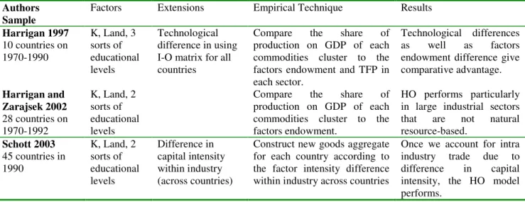
Like the first approach, the third approach analyzes the patterns of trade that are linked to factor endowments. This third approach (Table 1c), which we choose in this paper, is to compare factor endowments and trade in commodities as in equation 1.1.

(

)

1

c c c w

T = A− V −s V (1.1)

It was first developed by Leamer (1984) for two years, 1968 and 1975. One objective of such an estimation exercise is to infer implicitly the value of

Authors Sample

Factors Extensions Empirical Technique Results

Harrigan 1997 10 countries on 1970-1990 K, Land, 3 sorts of educational levels Technological difference in using I-O matrix for all countries

Compare the share of production on GDP of each commodities cluster to the factors endowment and TFP in each sector.

Technological differences as well as factors endowment difference give comparative advantage. Harrigan and Zarajsek 2002 28 countries on 1970-1992 K, Land, 2 sorts of educational levels

Compare the share of production on GDP of each commodities cluster to the factors endowment.

HO performs particularly in large industrial sectors that are not natural resource-based. Schott 2003 45 countries in 1990 K, Land, 2 sorts of educational levels Difference in capital intensity within industry (across countries)

Construct new goods aggregate for each country according to the factor intensity difference within industry across countries

Once we account for intra industry trade due to difference in capital intensity, the HO model performs.

1

A− (that is not directly measured) and to study how it changes over time. As for the commodities specialization test, this approach demands us to construct commodity clusters, which regroup products sharing the same technology.

In this paper we construct clusters differently than those used in previous studies to be more precise. This approach presents advantages because we only need data on endowment and trade, and not on technology in each product. Less data requirements makes it easier to carry out the analyses on a long time period (e.g. Lederman and Xu 2001). Because it does not make reference to factor intensity, it is a weakened form of the HOV model, what Feenstra (2004) calls the “partial” test. Curiously, this approach rarely relaxes assumptions of the HO model, except for Lederman and Xu (2001). Finally this type of approach allows us to obtain a large sample which is best to compare the role of endowment in factors and “new” determinants in explaining trade patterns.

Table 1c: Studies of net export patterns

Authors Sample

Factors Improvements Empirical Technique Results

Leamer 1984 27 countries 1958 and 1975 K, 3 sorts of land, 7 sorts of labor

Net exports by commodities clusters on relative factor’s endowments

Perform for natural resources intensive commodities Eastevardeorval 1997 18 countries in 1913 K, 2 sorts of Land, 2 sorts of educational levels

Net exports by commodities clusters on relative factor’s endowment

HO performs concerning the significance of relationship between factor endowment and net trade of goods. Lederman and Xu 2001 57 countries on 1970-1995 K, 3 sorts of land, 2 sorts of educational levels Difference in research and development Scale economics Consumers preferences Non linearity Trade impediments

Probability of being a net export for different commodities clusters on factors endowment, knowledge, ICT. And in a second step trade intensity for net importers and net exporters on scale effects or consumers preferences.

Land and capital play an important role on determining the status, but also other characteristics

2.2 Extensions to the strict HO theorem

As we have just seen, many assumptions on the HO theorem have been relaxed in previous studies. Let us look closely the theoretical implications of such relaxations. The HOV relation holds under the following: homogeneity in technology, constant scale returns, homothetic consumers’ preferences, non trade impediments. Otherwise, the relation between factors endowments and net export is not linear since it depends on the hypotheses that are relaxed. Which assumptions are relaxed in our study are discussed below.

Differences in technology: Factor content studies have shown us that similarity in technology is an assumption of the HOV model that must be relaxed to have a convenient test (Trefler 1995, Harrigan 1997, Davis and Weinstein 2001). Input output analyses among sectors between countries (Davis and Wenstein 2001, Schott 2003) have shown that factor intensity in sector varies across countries. This difference in technology could influence trade patterns in two ways. Firstly, concerning a neutral technology difference, it captures efficiency in the use of inputs, hence two countries with similar factors endowments but different inputs’ efficiency could have different patterns of trade9_{. Secondly, concerning a technology difference}

that changes factor proportion in sectors, it could provide a competitive advantage in the production of some specific goods10_{. Hence, let}

c

δ

measure the difference in factor productivity of each country. Compared to the standardA−1 (equation 1.3a), we obtain a new equation for net trade in commodities (equation 1.3b). 1 c c c Y ₌ A−

δ

V (1.3a) 9

In Trefler (1995), his preferred model use neutral technology difference across industries or factors which does not influence comparative advantage, so differences in technology are pure scale effects.

10

Neary (2003) using graphics shows that comparative advantage (determined by factors endowments) always explains trade structure. However, competitive advantage (in terms of productivity) has an impact on resource allocation, structure and volume of trade.

(

)

1

c c c c w

T A−

δ

V s V

= − (1.3b)

The impact of this difference in technology for specialization has been rarely tested empirically. Bowen and al. (1987) modify the HOV model by introducing differences in technology. And if they find that the original HOV model has a weak prediction, they reject as well differences in technology as a determinant. However, subsequently Trefler (1995) has shown that a model taking into account differences in technology between developed countries and developing countries improves substantially the empirical results of the original HOV model. On the other hand, in studies using the same test as we use in this paper (the weakness test), the difference in technology is never relaxed, except in the Lederman and Xu (2001), which controls for cross-country technological heterogeneity via unconvincing measures (research and development expenditures and stock of technical workers). Here we take into account differences in productivity via total factor productivity.

Homothetic preferences: Homothetic preferences in consumption also need to be relaxed. Hunter and Markusen (1988) provide convincing evidence that an assumption of quasi-homothetic preferences is superior to the traditional assumption of homotheticity. Bowen and al. (1987) find no evidence to relax such a restriction, but Markusen (1986) and Davis and Weinstein (2001) improve their factor content studies in considering non homothetic preferences. That is why in our study we include the mean income per capita11 _{as we consider an expanded version of the HO model}

by allowing a portion of consumption to be dependent on income (equation 1.4a). Under this more general formulation, if the endowment among two

11

Jones and al. (1998) explained clearly that in the case of intra-sectoral trade. A capital abundant country may import a more capital intensive good than this exported. Effectively whereas the traditional inter-sectoral factor intensity basis for trade relies primarily on supply-side differences between country in their endowments, the intra-sectoral pattern of trade reflect demand side differences

countries do not differ by much but demand patterns differ by more, a capital intensive country may export its relatively labor intensive commodities if its tastes are biased towards those commodities produced with more capital intensive techniques (equation 1.4b).

(Y/L) C =C so ( c c) c c Y L

s

=

s

(1.4a)

(

)

1 ( c c) c c c c w Y L T ₌A−

δ

V ₋s V (1.4b)

Returns to scale: The assumption of constant returns to scale should also be relaxed. Returns to scale are not constant across sectors. Large countries have low autarkic price in sectors where scale economies are important (with increasing returns). Therefore, these countries have a comparative advantage in the international market for specific sectors with increasing returns to scale. Markusen and Melvin (1981) develop a model where in equilibrium a large country exports the commodity with increasing returns to scale and the other countries export the commodities with constant returns to scale. Antweiler and Trefler (2002) in a factor content version find that allowing for the presence of increasing returns to scale in production significantly increases our ability to predict international factor services trade flows. They find that a third of all goods-producing industries are characterized by increasing returns to scale12_.

Since scale likely includes aspects of international technology differences13_,

it is important to use a measure which is not directly related to factor productivity. Here we adopt the Lederman and Xu (2001) technique of adding as determinant of trade patterns a measure of scale in the economy (population) to see which sort of products are sensible to increasing returns

12

These increasing returns to scale factors content prediction have rarely been explored empirically. Leamer (1984) admits that it is “a great disappointment” that his work does not deal seriously with economies of scale

13

In Antweiler and Trefler (2002), the industries with the largest scale estimates are mostly those where technical change has been most rapid. New process technologies are often embodied in larger plants.

to scale14_{. We use the formulation of Antweiler and Trefler (2002)}

where

µ

is the elasticity of scale in each sectors (equation 1.5a). Contrary to technological differences which are specific to each country, increasing scale returns are specific to sectors.

( )

1

(

)

( _c/ _c) c c c c w Y L T

µ

A−

δ

V s V = − (1.5a)

Trade impediments: Frictions (trade barriers15_{, transaction and}

transport costs) should also be taken into account. As Leamer (1984) showed, these impediments are reflected in a deviation of domestic prices from international prices. Davis and Weinstein (2001) improve the HOV model in adding a measure of trade costs through a gravity equation. We control for landlockness and distance to the market16_{, which could increase}

transport costs. We also control for the difference in infrastructure and ICT endowment, and we take into account the intensity of free trade by using a measure of deviation from predicted trade, to measure trade barriers. We introduce the price differences notion in our formulation: let

θ

, the price difference to the world price due to transport cost, tariffs and other trade impediments. We express trade and resources in value terms.

In matrix notation, let θ subscript indicate variables that depend on trade impediments, w the vector of factor prices and p the vector of commodity prices. Then, the zero profit condition Aw= p

becomesA w_{θ θ} =

θ

pw = p_θ. Hence, the production evaluated at the internal prices is Yc =A w V−1 _θ c and the consumption at internal prices is

C

c

s Y

c w

θ

=

.

Let w V_θ c, be the vector of resources evaluated at the internal prices, and

14

Trefler (2002) remarked, it seems unusual that we do not distinguish between internal and external returns to scale, as their different in their implications for market structure and trade patterns. But Helpman and Krugman (1985) help us in showing that the form of scale has only very modest implications for the factor content of trade.

15

Travis (1964) argues that tariffs on labor intensive imports can explain the Leontief finding that US in 1947 was net exporter of labor services.

16

w w

w V , the vector of world resources evaluated at the world prices. We may then write the trade vector in value terms as:

( )

(

( )

)

1 / c c c c c c w w Y L p T_θ

µ

A_θ− w_θ

δ

V s_θ w V = − (1.6) 3. Empirical approach

This part presents econometric results about the determinants of trade structure and trade intensity across countries and over time. These estimates control for the simultaneous determination of the intensity of trade (that is, the level of net exports) together with a non-linear version of comparative advantage models. More specifically, we model export intensity as a Heckman selection model. That is, country-specific characteristics or factor endowments determine comparative advantage (proxied by the condition of having positive net exports), and then domestic and foreign market sizes, the macroeconomic environment, transaction costs, and institutions determine export intensity. Moreover, we allow the estimates of trade intensity for the importer and the net-exporter sub-samples to differ.

3.1 A selection model

To implement equation (1.6) one could regress the net exports of a country c for a product i in year t,NXict, on endowment in different factors j,Ejct,

on k new determinants (difference in productivity, in consumers preferences and returns to scale) Nkct, on m variables determining trade

intensity (or impediments) TImct and on regional dummies DRrt and year

0 1 2 3 1,5 1,3 1,5 ict j jct k kct M mct rt t ct j k m

NX

β

β

E

β

N

β

TI

DR

DY

ε

= = =

=

+

∑

+

∑

+

∑

+

+

+

(2.1)

However trade impediments variables will not have the same impact on net trade for net importers and net exporters, since trade liberalization increases the net trade ratio for net importers and decreases the net trade ratio for net exporters. So in a linear homogenous implementation, the effects of many variables are washed out by this heterogeneity. In other words, it is unlikely that the coefficients of the explanatory variables for trade intensity are the same for all countries, especially for importing and exporting countries of the same commodity. If we consider that the impact of trade intensity differs according to the status for a country (e.g. increase (decrease) net exports for net exporter (net importer), we have to add the trade intensity variables interacted with a dummy indicating the status Sct of the country (where 1 indicate a net

exporter and 0 a net importer). And the status of countries, net exporter or net importer, depends mainly on factors endowments but also on technology, consumers’ preferences and scale effects.

However once we account for the status, factor endowments does not matter on the volume of tradeNXict. Neary (2003) shows that

comparative advantage in factors endowments continues to determine direction of trade (the specialization) however competitive and absolute advantage due to productivity or scale effects impact on trade patterns and trade volume. So factors endowments do not appear in our second step on net trade volume; they impact only on the status. An estimable model would have the following form:

_{0 1 2 3 4} 1,3 1,5 1,5 ( * ) ict k kct M ct mct M mct M ct t ct k m m NX β β N β S TI β TI β S DY ε = = = = +

∑

+

∑

+

∑

+ + + (2.2)

where 0 1 2 1,5 1,3 ct j jct k kct rt t ct j k S α α E α N DR DY µ = = = +

∑

+

∑

+ + + (2.3) with

β

₂

>

0

and

β

₃ <0

But in using a probit estimation for the status, this implies that the relationship between factor endowment and the net export is not linear. The initial presumed linear relationship between factor endowments and the structure of net exports is questionable (Leamer 1984, Leamer et Levinsohn 1995). Effectively all countries do not produce all goods, particularly developing countries. An increase in capital endowment would not lead to an increase in capital-intensive good exports if the country is already specialized in a non capital intensive good or does not product a capital intensive.

As Leamer (1995), we present our data in Figure 1 below which plots net exports of a labor-intensive aggregate composed mostly of apparel and footwear divided by the country’s workforce against the country’s overall capital/labor ratio. There is very clear evidence of nonlinearity here – countries which are very scarce in capital don’t engage in much trade in these products. Exports start to emerge when the capital/labor abundance ratio is around $10,000 per worker.

ARG AUT BDI_BENBGD BLZ BOL BRA CAF CAN CHE CHL CHN CMRCOG COL_CRI

CZE DNK DZA ECU EGY ESP FIN FRA GAB GBR GHA GRC GRD GTM HND HUN IDN IND IRL ISL ISR ITA JAM JPN KEN KOR LKA MAR MDG _MEX MOZ MUS MWI MYS NGANIC NLD NOR PAK PAN PER PHL PNG POL PRT PRY SDN SEN SGP SLV SWE SYC SYR TGO THA TTO TUNTUR UGA URY USA VEN

VUTWSMZAF YUG

ZWE −1500 −1000 −500 0 500 1000

Net Export per Worker ($)

0 20000 40000 60000 80000 100000

Capital per Worker ($)

Net Export of Labor Intensive Manufacture per Workers vs Capital per Workers (1990)

Figure 1

Exports rise to around $300 per worker when the country’s abundance ratio is around $20,000 per worker. Thereafter, net exports steadily decline, turning negative when the country’s capital/labor abundance ratio is around $40,000. Hence until a sufficient level of capital per worker, an increase in capital per worker has no effect on specialization.

With a probit estimation we have a non linear relationship, meaning that the marginal impact of an increase in factor endowment is greater when the factor endowment is sufficiently high to allow countries to be specialized in the good. So we are confident in our assumption concerning non linearity between factor endowment and trade structure.

With a linear estimation, we would have biased results in case of correlation between

ε

ct and

µ

ct. It is plausible that the unobservable

variables for the status would be correlated with unobservable variables for the amount of net exports. Following Lederman and Xu (2001), we use a

Heckman procedure to control for that. As shown in Figure 2, we initially test in equation 2.4 the probability of being a net exporter of a good (i.e. the status). We assume that the probability of having positive net exports Sct is

determined by the conventional explanatory variables, factor endowmentsEjct (arrow 1), and by ‘new” determinants Nkct (arrow 2).

Contrary to Lederman and Xu (2001), we assume increasing returns to scale and differences in consumers’ preferences as potentials determinants in this comparative advantage equation. Moreover some determinants of trade intensity TImct (e.g. infrastructure and ICT) could also determine

comparative advantage (arrow 3), since products are differently sensitive to transport and transactions costs17_.

0 1 2 3 1,5 1,3 1,2 ct j jct k kct m mct rt t ct j k m S α α E α N α TI DR DY µ = = = = +

∑

+

∑

+

∑

+ + + (2.4) 1 4 3

+

=

2 5 Net Exporter or Net Importer ct S Trade Intensity ict NX Trade Flows HOV: Factor’s Endowment (Capital, Land, Human Capital) jct E News determinants: Technology, Scale Returns, Consumer’s preferences kct N

Trade policy, Country’s size, Landlockness, Growth of partners,, Infrastructure, ICT mct TI 17

In a Heckman procedure all determinants of the second step (here trade intensity variables) have to be included in the first step if they are significant in this first step. The same variables that determine how big a country's net exports of a particular good (or commodity group) also determine that probability that a country will export these goods at all.

Figure 2

Then we continue by testing the explanatory variables on the samples of net exporters (equation 2.5) and net importers (equation 2.6) relative to trade intensity (Figure 2). To the usual determinant of trade intensity (arrow 4), we add new determinants that are as important as in comparative advantage (arrow 5). This procedure permits to uncover a trade intensity trend, since, without separating the sample into net importers and net exporters, it cannot appear. Effectively an increase in trade will raise net exports in the net exporters segment and the net imports in the net importers segment, therefore on a global sample the effect on net export would be null.

0 1 2 1,3 1,5 if S=1 ict k kct M mct t ct k m NX β β N β TI DY ε = = = +

∑

+

∑

+ + (2.5) _{0 1 2} 1,3 1,5 if S=0 ict k kct M mct t ct k m NX β β N β TI DY ε = = = +

∑

+

∑

+ + (2.6)

This specification is acceptable only if we add variables in the first step that do not appear in the second step to identify our model. Those variables are factor endowments and regional dummies. Our justification is both theoretical and statistical. Firstly as we said before, we do not expect a linear relation between relative factor endowment and net export intensity18_{. Secondly, from a statistical standpoint, we see in the Table A1}

(in Annex) that the condition of being a net exporter has an even higher cross-country variance (column “between”) relative to cross-time variance (column “within”) than the value of net export for most sectors. The relative factor endowment variables (in bold) are also relatively more stable over time than among countries.

3.2 Construction and measure for commodities’ clusters

18

When we add factor endowment ratios in the second equation we obtain non significant or non sensible results.

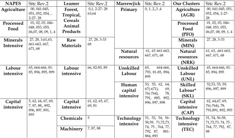
In order to divide the products into different categories (Table 2), we drew our inspiration from Leamer (1984) whose classification is often used in other studies (Estervadeordal 1997, Lederman and Xu 2001) from the NAPES’ classification and from the factor intensity classification of Marrewjik (2004) on the basis of UNCTAD/WTO and ITC classification. Our classification (Table 3) is less detailed than Leamer’s with regard to the categories of primary products for which the determinants of comparative advantage have often been estimated. We construct three clusters of primary products, agricultural products (AGR), processed food products (PFO) and Minerals products (MIN).

We increase the number of categories of manufactured goods by using a 3-digit classification, in order to distinguish human capital intensive products, which was not allowed in Leamer’s classification. We obtain five clusters for manufactured products: intensive in natural resources and capital (NRK), intensive in unskilled labor (UNL), intensive in skilled labor (SKL), intensive in capital (CAP) and intensive in technology (TEC). This level of detail is more precise compared to the existing literature; which should allow us to obtain better results than using only a two digit classification.

Table 2: Construction of clusters

NAPES Sitc Rev.2 Leamer Sitc Rev.2 Marrewjick Sitc Rev.2 Our Clusters Sitc Rev.2 Agriculture 00, 041-045, 051, 052, 054, , 2-27- 28 Agriculture (AGR) 00, 041-045, 051, 052, 054, 2-27- 28 Processed Food 01, 02, 03, 046-048, 053, 055, 06,07, 08, 09, 1, 4 Forest, Tropical, Cereals Animal Products 0,1, 2-27- 28 63,64 Processed Food (PFO) 01, 02, 03, 046-048, 053, 055, 06,07, 08, 09, 1, 4 Primary 0, 1, 2,,3 ,4 Minerals (MIN) 27, 28, 3-33 Minerals Intensive 27, 28, 3,61,63, 661-663, 667, 671, 68 Raw Materials 27, 28, 3-33 68 Natural resources 61, 63 661-663, 667, 671, 68 _resources Natural (NRK) 61, 63, ,661-663, 667, 671, 68 Unskilled Labour 65, 664-666, 793, 81-85, 894, 895 Unskilled Labour (UNL) 65, 664-666, 81-85, 894, 895 Labour intensive 65, 664-666, 81-85, 894, 895, 899 _intensive Labour 66, 82-85, 89 Skilled Labour* (SKL) 52,53, 55, 59, 896, 897, 899 Capital intensive 61, 62, 65, 67, 69, 81 Human capital intensive 53, 55, 62, 64, 67(-671), 69, 76(-764), 78, 791, 885, 892, 896, 897, 898 Capital intensive (CAP) 62, 64,67, 69, 76(-764), 78, 791,891, 892, 893 Chemicals 5 Capital intensive 5, 62, 64, 67, 69, 7, 87, 88,, 892, 896, 897, 891, 893 Machinery 7, 87, 88 Technology intensive 51, 52, 54, 56-58,59, 71,72,73, 74, 75 , 764, 77, 792, 87, 881-884, 893 Technology intensive (TEC) 51, 54, 56-58, 71,72,73, 74, 75 , 764, 77, 792, 87, 88

*We use Marrewijck(2004) and Estervadeordal (1997) approach for this cluster. Because of the incertitude on the form of the relationship between factor endowments and trade structure (linear or not), I used several specifications to measure trade structure. Sometimes gross exports are used. Deardoff (1984) clearly prefers to use the net exports indicator, arguing that if there are differences with gross exports results, it will be due to intra industry trade about which H-O theorem does not reach a decision. We follow Leamer (1988) approach and for selected clusters, we use the share of net exports on GDP. This ratio being negative for net importers, we added a constant to allow us to use a logarithm form. We finally obtain a sample of 71 countries on 1960-2000.

3.3 Construction and measure for factors endowments

The HO model framework considers relative factor endowment between many factors but also between many countries. Factor intensity in a country is often measured as factor intensity in a sector, i.e. by a ratio of the factor on labor as denominator for the most reliable studies; otherwise some only use the stock of the factor. It is more suitable to use a ratio of per capita endowment of a factor in the country to the world per capita endowment of this factor as we deal with relative advantage in factor endowment (Harrigan and Zakrajsek, 2002). We use the formula constructed by Spilimbergo and al. (1999)19_{. The ratios are weighted by the}

degree of openness to take into account that endowments of closed countries do not compete in the world markets with other factors.

The factor content studies mainly used occupational-based classification to measure human capital endowments. We prefer to use an educational-based classification for the reasons exposed by Harrigan (1997). The first is that educational levels are more likely to be exogenous with respect to net exports shares, since growth in some industries might induce workers to shift their occupations. The second is that education is probably more closely related to skill than occupation. However, rather than using a secondary school enrolment rate (lagged six years) as Balassa and Bauwens (1986) did, we prefer to use as Harrigan and Zakrasejk (2000), stock measures of education of the current labor force calculated from the Barro and Lee database (2000). In contrast to Estervadeordal (1997) or

19

if

E is the endowment of country i in factor f and the measure of relative endowment is

( )

( )

* ln f if if E E RE = and * if i i i f i i i X M E pop GDP E X M pop GDP  _{ + } × ×        =   ₊  ×       

∑

∑

Schott (2003) who used only the distinction between skilled and unskilled workers, we use, as Harrigan (1997) three sorts of skill: unskilled, primary skilled and highly skilled.

Physical capital is difficult to include because of its mobility. Wood (1994) argues that empirical tests of the H-O model were mispecified by considering physical capital as the land while it is more mobile across countries and should not affect the structure of net exports across countries. However, the well-known Ethier-Svensson-Gaisford (ESG) model with mobile (capital) and immobile (land and labor) factors shows that capital is a determinant of pattern of trade for a country, depending on capital intensity of the goods in which its immobile factors give it a comparative advantage. Thus if a country has a high labor-land ratio, making it an exporter of clothing, which happens to be also capital intensive, then it exports capital via goods and capital affects the pattern of trade. But if it has a low labor-land ratio, making it an exporter a less capital-intensive goods (e.g. food), then it exports capital directly (by Foreign Direct Investment). Following Leamer (1999), we adopt the Kraay and al. (1999) measure of capital stock per worker.

The measure for natural resources is arable land per habitant, so our measure does not include resources in mineral and fuel which are not available for a large sample in the period under review. The only measure available for our sample is the index from Isham and al. (2005) based on the net export ratio in mining and fuel products, so we could not use it in an estimation of net exports in mineral products due to endogeneity issues.

3.4 Construction and measure of “new” determinants of trade

Concerning differences in technology, we measure total factor productivity (TFP). This measure was used by Harrigan (1997) to explain how differences in technology associated to factor endowments could help

to explain specialization in production. We use the TFP index of Bosworth and Collins (2003) who calculate the residual of a growth regression (assuming constant returns to scale). We use a proxy of scale economic effect that could lead the country to be specialized in some increasing returns to scale sectors, measured by the number of habitants. We control also for differences in consumer’s preferences via income per habitant, since an increase of per capita income will lead the consumer to prefer capital and human intensive goods and hence to be a net importer of this commodity.

3.5 Construction and measure of trade intensity explanatory variables

Variables that determine trade intensity can be separated in two groups: structural variables and the political variables. The first ones are the distance to its main partners, and the size of the domestic market, which is measured by population and GDP per habitant. Domestic transport infrastructure and transaction costs determine the amount that a country exports or imports. For those variables, we use an index constructed as a principal component (roads networks, rails networks and paved road for infrastructure; personal computer, internet host, telephone lines and mobile phones for ICT). Finally openness depends on the degree of outwardness for the country. We measure this position by an indicator computed from the method proposed by Guillaumont (1994). We measure the part of trade that is not explained by domestic market size (population), landlockness, mean income in the country, to be an OCDE country and to be an oil exporter20_{. Since we use generated variables (openness policy,}

mills ratio, principal component index) we have to recalculate all the

20

( ) ( ) ( ) ( ) ( )

** *** *** ***

ln X M 11.68 0.09 ln PIB t/ 0.25 ln Pop 0.50 ln Dist 0.05 encl 0.07 ln Xpétrole

PIB ε +   = + − − − + +    

standards errors of the variables, we use the bootstrap technique to estimate standard errors and to construct confidence intervals21_.

4 Results

The main objective of this study is to improve the prediction of patterns of trade. So we have to assess the reliability of the prediction of status for each country. This is done in section 3.1. We have also a large part of this paper on the importance of “new” determinants of comparative advantage. In section 3.2, using an Anova estimate, we compare their importance relative to the traditional factors and we analyze changes during two periods, 1960-1980 and 1960-1980-2000. Then we comment on the results of the Heckman estimation. In section 3.3 we present results for the first step, the selection equation on comparative advantage, which is estimated for two periods. The last section, 3.4, deals with the second step, trade intensity. We jointly comment results on net exporter and on net importer of each cluster.

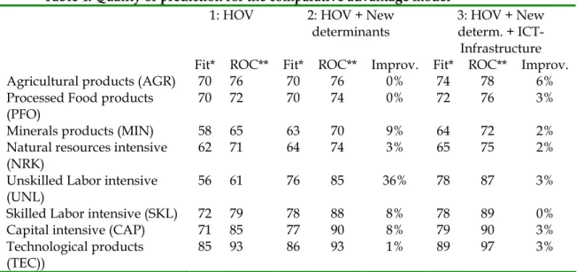
4.1 Goodness of fit

A way to assess model fit is to concentrate on its predictive power by looking at prediction statistics. In the first part of table 4 we present the goodness of fit for a model with only factor endowments. In the second part, we add new factors (productivity differences, scale returns and consumers preferences) and in the last part we add ICT and infrastructure. For each part, the first column gives us the predictive success rate calculated with the sensitivity, percentage of positive sign (net exporter) correctly identified, and the specificity, percentage of negative sign (net

21

For a generated variable, the confidence interval in the second step is not correct as it refers to the first step. So we built a sampling distribution based on the initial sample from which repeated sample are drawn to obtain a correct distribution and correct standards errors.

importer) correctly identified. We add in the second column a test which compares the predicted results to a random assignment. For the second and third parts, the third column presents the improvement in the goodness of fit (measured by the Fit test) compared to the previous part. For example, for the capital intensive cluster (CAP), accounting for new determinants improves the goodness of fit by 8%, and if we account for difference in ICT and Infrastructure we improve the goodness of fit by 3%.

Table 4: Quality of prediction for the comparative advantage model

1: HOV 2: HOV + New

determinants

3: HOV + New determ. +

ICT-Infrastructure Fit* ROC** Fit* ROC** Improv. Fit* ROC** Improv.

Agricultural products (AGR) 70 76 70 76 0% 74 78 6%

Processed Food products (PFO)

70 72 70 74 0% 72 76 3%

Minerals products (MIN) 58 65 63 70 9% 64 72 2%

Natural resources intensive (NRK)

62 71 64 74 3% 65 75 2%

Unskilled Labor intensive (UNL)

56 61 76 85 36% 78 87 3%

Skilled Labor intensive (SKL) 72 79 78 88 8% 78 89 0%

Capital intensive (CAP) 71 85 77 90 8% 79 90 3%

Technological products (TEC))

85 93 86 93 1% 89 97 3%

* Proportion of correct sign prediction for net exporters and net importers (with the mean of predicted probability as cutoff). ** Receiver Operating Characteristics: Compared to a random prediction (50 means that the model doesn’t do any better that random assignment would).

We conclude that adding “new” determinants for trade patterns helps us to improve the prediction to be a net exporter for manufactured products as well as for minerals products. Improvement due to the inclusion of ICT and infrastructure seems to concern all clusters, and especially primary commodity cluster.

As a comparison, in Bowen and al. (1987) the sign test22 _{is around 0.6 (it}

depends on factors). Trefler (1995) with the sign test improves his model from 0.71 (conventional factors) to 0.93 (conventional and “new” determinants). Davis and Weinstein (2001) with the same test improve their model from 0.32 to 0.91. Antweiler and Trefler (2002) obtained a sign test of 0.67 with a strict HOV model and 0.66 with a modification taking into account returns to scale. Here the percentage of signs correctly identified depends on sectors; the”new” determinants do not improve the ROC test for primary and high technology products.

22

Proportion of observations for which excess in factor endowments and excess in factor content in net export have the same sign.

Because of the presence of a number of potentially collinear variables in this first step we implement the variance inflation factor test (VIF). The literature states that in order for an indication of multicolinearity to exist, the value that indicates the highest VIF should be greater than 5. Here we have 4.7 which suggest that multicolinearity is not a serious problem.

4.2 Conventional factors versus “new” factors: ANOVA estimates

As we see in the ANOVA exercises23 _{on the predicted probability of being}

a net exporter of a product (in table 5), the role of conventional factors in accounting for patterns of comparative advantage is still important. However concerning some industrial products the new factors could be more important to explain structure of trade. In the conventional factors we add a distinction between capital and land on one hand, and human capital on the other hand, which is sometimes analyzed as a non conventional factor (Lederman and Xu 2001). We perform this test on two periods, 1960-1980 and 1960-1980-2000.

23

We report the range of the variance of comparative advantage attributable to traditional factors and to “new” factors.

Table 5: Role of Conventional and New factors in explaining the predicted probabilitya

Share of variance explained by:

Period Land and Capital Human Capital New ICT-Infra R squared Agricultural products 1960-2000 24% 32% 4% 41% 98 AGR 1960-1980 15% 15% 3% 67% 1980-2000 41% 40% 13% 7% Processed Food 1960-2000 48% 37% 11% 4% 96 PFO 1960-1980 44% 41% 10% 5% 1980-2000 47% 41% 10% 3%

Minerals (raw, without oil) 1960-2000 39% 39% 8% 14% 99

MIN 1960-1980 25% 56% 4% 16%

1980-2000 47% 17% 7% 30%

Natural Resources Intensive 1960-2000 54% 32% 6% 8% 91

NRK 1960-1980 27% 37% 10% 25%

1980-2000 50% 33% 4% 13%

Unskilled Labor intensive 1960-2000 5% 17% 65% 13% 88

UNL 1960-1980 5% 14% 70% 11%

1980-2000 8% 45% 41% 6%

Skilled Labor intensive 1960-2000 26% 5% 60% 9% 81

SKL 1960-1980 30% 24% 43% 3% 1980-2000 13% 5% 65% 16% Capital intensive 1960-2000 1% 49% 42% 8% 79 CAP 1960-1980 2% 52% 43% 3% 1980-2000 4% 50% 41% 6% Technological products 1960-2000 39% 25% 26% 10% 67 TEC 1960-1980 21% 26% 46% 8% 1980-2000 50% 25% 15% 10%

a _{The dependent variable in the ANOVA equations is the predicted probability of}

being a net exporter of the product.

As we could expect, physical capital endowments is not a main determinant to explain the choice of specialization across industrial clusters. Because of its mobility, a country which has more capital could prefer to transfer it in another country via FDI rather than invest it in a more capital intensive production. In the same way a country relatively less endowed in physical capital could produce more capital intensive goods via FDI from another country. Roughly for primary products the share of traditional factors is greater than the share of new determinants, and inversely for manufactured goods.

The main conclusion about the decomposition in two periods is that effectively conventional factors are not the only determinants of trade patterns but they are as determining as ever during the specialization that took place during the least twenty years. Land abundance is particularly more determining in the last period for primary products, because of the emergence of land abundant developing countries in international trade.

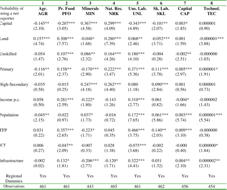
4.3 Comparative advantage

The role of Conventional factors

Concerning natural resources, results are encouraging because of the positive and significant sign for the probability of being a net exporter of AGR, PFO and NRK. The results in table 6 imply that a one percent increase in the relative endowment in arable land is associated with an increase in the probability of being a net exporter of PFO of 0.308% (column 2) and of 0.28% for NRK (column 4). Those results confirm earlier estimated found by Leamer (1984), Estervadeordal (1997), Lederman and Xu (2001). The non significance for MIN (column 3) is probably due to the misspecification of endowment in mineral resources (we just measure endowment in arable land). The negative coefficient for land abundance concerning TEC (column 8) conforms to Leamer’s view (1999) that countries relatively abundant in land will export land intensive products and after extracting the capital used in agriculture their capital abundance ratio is less than that of countries not relatively abundant in land24_.

In the case of the capital stock, here again we have good results. The positive sign on MIN and NRK (columns 3 and 4) conforms to the characteristics of those sectors. These results contradict those from Leamer (1984) and Lederman and Xu (2001), but conform to Estervadeordal’s

24

Leamer explains in this why US in 1947 were a net importer of capital intensive goods from Japan whereas US were more capital intensive than Japan.

results (1997). Concerning manufactured commodities, no study found a significant impact of endowment in capital on labor intensive goods and capital intensive goods25_{. Here by discerning more clusters we find a}

negative impact on UNL (column 5) and SKL (column 6) and a positive (but weak) impact on CAP (column 7).

Previous studies did not obtain good results on the human capital component. Estervadeordal (1997) found that skilled labor was significantly positive as well as labor intensive goods as capital intensive goods; Lederman and Xu (2001) found that it was significantly negative for all manufactured goods. In discerning three sorts of skills we obtain relatively better results, and the results roughly conform to expectations. An increase in the share of non educated labor or primary educated labor increases the probability of being a net exporter of UNL intensive products. We observe the increase in this probability is greater for a 1% increase in the share of primary educated labor (+0.37%) than for a 1% increase in the share of non educated (+0.18%) meaning that UNL intensive sector needs more primary educated labor than non educated labor.

The coefficients appearing in the table are marginal effects calculated for the mean value of the variable. However we assumed a non linear relationship, that is an impact of an increase in capital per labor which differs according to the value of this variable. In the annex we show graphs (Graphs A) for the results of an increase in different factors on the probability of being a net exporter of different groups of products intensive in the factor. We can observe that the impact of increasing the endowment in a factor has no impact until a sufficient level of endowment, hence the

25

In Estervadeordal and Leamer, the impact was positive in the two cases, in Lederman and Xu, the impact was negative on labor intensive goods but non significant on capital intensive goods.

impact if stringer until a point where additional endowment do not play anymore on the probability becoming net exporter.

Table 6: Determinants of Comparative Advantage: Heckman selection equation: Probit on the probability of being a net exporter of each commodity cluster on 1960-2000. 1 2 3 4 5 6 7 8 Probability of being a net exporter Agr. AGR Pr. Food PFO Minerals MIN Nat. Res. NRK Uns. Lab. UNL Sk. Lab. SKL Capital CAP Technol. TEC Capital -0.145** -0.207*** 0.367*** 0.299*** -0.343*** -0.101** 0.003* 0.000001 (2.10) (3.05) (4.58) (4.09) (4.89) (2.07) (1.85) (0.90) Land 0.157*** 0.308*** -0.048* 0.280*** 0.068** -0.052*** 0.001 -0.000001*** (4.74) (7.57) (1.68) (7.39) (2.46) (3.71) (1.59) (3.88) Unskilled -0.054 0.107*** 0.086** 0.164*** 0.180*** -0.004 -0.002** -0.000000 (1.47) (2.76) (2.32) (4.26) (4.10) (0.28) (2.51) (1.03) Primary -0.116** 0.158** -0.170*** 0.222*** 0.371*** 0.111*** 0.005*** 0.000001* (2.01) (2.37) (2.90) (3.47) (5.36) (3.78) (2.97) (1.91) High-Secondary -0.035 -0.015 0.247*** 0.262*** 0.080 0.090*** 0.001 0.000001 (0.58) (0.25) (4.18) (4.40) (1.18) (2.84) (0.56) (0.73) Income p.c. 0.058 0.281*** -0.222* -0.143 0.310*** 0.061 -0.004* -0.000002 (0.50) (2.59) (1.80) (1.26) (2.77) (0.82) (1.66) (1.43) Population -0.045** -0.022 0.037* -0.016 0.172*** 0.061*** 0.003*** 0.000001*** (2.15) (0.97) (1.73) (0.72) (7.65) (5.86) (5.74) (5.54) TFP 0.031 0.357*** -0.223* 0.045 0.466*** 0.140** 0.009*** -0.000000 (0.22) (2.65) (1.71) (0.35) (3.75) (2.03) (3.10) (0.38) ICT _{0.006 -0.047** -0.007 0.028 -0.075*** -0.002 -0.000 0.000000*} (0.27) (2.09) (0.33) (1.38) (3.68) (0.22) (0.40) (1.84) Infrastructure -0.002 0.132* -0.206*** -0.120* 0.322*** 0.051 0.004** 0.000002** (0.02) (1.81) (2.77) (1.71) (4.41) (1.32) (2.10) (2.31) Regional Dummies

Yes Yes Yes Yes Yes Yes Yes Yes

Observations _{461 461 443 465 461 462 456 454}

The coefficients are the marginal coefficients.

We can conclude by the distinction between the two periods (Table 7 in Annex) that the impact of skill seems more conform to the theory in the second period than in the first one, especially concerning AGR, PFO, MIN and NRK sectors. Concerning these sectors, to be well endowed in