HAL Id: hal-01197334
https://hal.archives-ouvertes.fr/hal-01197334
Submitted on 11 Sep 2015HAL is a multi-disciplinary open access archive for the deposit and dissemination of sci-entific research documents, whether they are pub-lished or not. The documents may come from teaching and research institutions in France or abroad, or from public or private research centers.
L’archive ouverte pluridisciplinaire HAL, est destinée au dépôt et à la diffusion de documents scientifiques de niveau recherche, publiés ou non, émanant des établissements d’enseignement et de recherche français ou étrangers, des laboratoires publics ou privés.
Coherent manipulation of Andreev states in
superconducting atomic contacts
C Janvier, L Tosi, L Bretheau, Ç. Ö. Girit, M Stern, P Bertet, P Joyez, D
Vion, D Esteve, M.F. Goffman, et al.
To cite this version:
C Janvier, L Tosi, L Bretheau, Ç. Ö. Girit, M Stern, et al.. Coherent manipulation of Andreev states in superconducting atomic contacts. Science, American Association for the Advancement of Science, 2015, 349 (6253), pp.1199. �10.1126/science.aab2179�. �hal-01197334�
1
Coherent manipulation of Andreev states
in superconducting atomic contacts
C. Janvier1, L. Tosi1,2, L. Bretheau1†, Ç. Ö. Girit1††, M. Stern1, P. Bertet1, P. Joyez1, D. Vion1, D. Esteve1, M. F. Goffman1, H. Pothier1, C. Urbina1*.
1
Quantronics Group, Service de Physique de l’État Condensé (CNRS UMR 3680), IRAMIS, CEA-Saclay, 91191 Gif-sur-Yvette, France
2
Centro Atómico Bariloche and Instituto Balseiro, Comisión Nacional de Energía Atómica (CNEA), 8400 Bariloche, Argentina
†
Present address: Department of Physics, Massachusetts Institute of Technology, Cambridge, Massachusetts 02215, USA
††
Present address: CNRS USR 3573, Collège de France, 11 place Marcelin Berthelot, 75005 Paris, France
*Correspondence to: cristian.urbina@cea.fr
Abstract:
Coherent control of quantum states has been demonstrated in a variety of superconducting
devices. In all these devices, the variables that are manipulated are collective electromagnetic
degrees of freedom: charge, superconducting phase, or flux. Here, we demonstrate the
coherent manipulation of a quantum system based on Andreev bound states, which are
microscopic quasiparticle states inherent to superconducting weak links. Using a circuit
quantum electrodynamics setup we perform single-shot readout of this “Andreev qubit”. We
determine its excited state lifetime and coherence time to be in the microsecond range.
Quantum jumps and parity switchings are observed in continuous measurements. In addition
to possible quantum information applications, such Andreev qubits are a testbed for the
2
The ground state of a uniform superconductor is a many-body coherent state. Microscopic
excitations of this superconducting condensate, which can be created for example by the
absorption of photons of high enough energy, are delocalized and incoherent because they
have energies in a continuum of states. Localized states arise in situations where the
superconducting gap Δ or the superconducting phase undergo strong spatial variations:
examples include Shiba states around magnetic impurities (1), Andreev states in vortices (2)
or in weak links between two superconductors (3). Because they have discrete energies
within the gap, Andreev states are expected to be amenable to coherent manipulation
(4,5,6,7,8). In the simplest weak link, a single conduction channel shorter than the
superconducting coherence length , there are only two Andreev levels
2, 1 sin ( / 2)
A
E
, governed by the transmission probability of electrons through the channel and the phase difference
between the two superconducting condensates (3). Despite the absence of actual barriers, quasiparticles (bogoliubons)occupying these Andreev levels are localized over a distance around the weak link by the gradient of the superconducting phase, and the system can be considered an “Andreev
quantum dot” (5,6). Figure 1 shows the energies Ei
of the different states of this dot. In the spin-singlet ground state g only the negative energy Andreev level is occupied and
g A
E E . If a single quasiparticle is added, the dot reaches a spin-degenerate odd-parity
state o with Eo 0 (9-12). Adding a second quasiparticle of opposite spin to the dot in
state o brings it to a spin-singlet even-parity excited state e with Ee EA (13,14). The
e state can also be reached directly from g by absorption of a photon of energy 2EA.
Here we demonstrate experimentally the manipulation of coherent superpositions of states
3
Atomic-size contacts are suitable systems to address the Andreev physics because
they accommodate a small number of short conduction channels (15). We create them using
the microfabricated break-junction technique (16). Figure 2 presents the sample used in the
experiment. An aluminum loop with a narrow suspended constriction (Fig. 2C) is fabricated
on a polyimide flexible substrate mounted on a bending mechanism cooled down to 30 mK
(17). The substrate is first bent until the bridge breaks. Subsequent fine-tuning of the bending
allows creating different atomic contacts and adjusting the transmission probability of their
channels. The magnetic flux threading the loop controls the phase drop
2
0across the contact and thereby the Andreev transition frequency fA( , )
2EA/h (
0 is theflux quantum, h Plank’s constant). To excite and probe the Andreev dot, the loop is
inductively coupled to a niobium quarter-wavelength microwave resonator (17) (Fig. 2B) in a
circuit quantum electrodynamics architecture (18,19). The resonator is probed by
reflectometry at frequency f0 close to its bare resonance frequency fR 10.134GHz. The
actual resonator frequency is different for each one of the three Andreev dot states: in the odd
state, the resonance frequency is unaltered while the two even states lead to opposite shifts
around fR (20). The Andreev transition g e is driven using a second tone of frequency
1
f . Details of the setup are shown in figures S1 and S2 (20).
Here we present data obtained on a representative atomic contact containing only one
high transmission channel. Data from other contacts is shown in figures S6-S8. First, a
two-tone spectroscopy is performed by applying a 13 µs driving pulse of variable frequency,
immediately followed by a 1 µs-long measurement pulse
f0 10.1337 GHz
probing theresonator with an amplitude corresponding to an average number of photons n 30 (see
4
to the Andreev transition. The spectrum is periodic in flux, with period
0, which allows calibrating the value of across the contact (Fig. S3). Fits of the measured lines for different contacts with the analytical form of fA( , )
provide the transmission probability of highly transmitting channels with up to five significant digits, as well as the superconducting gap/h 44.3 GHz
of the aluminum electrodes.
The coupling between the resonator and the Andreev dot is evident from the avoided
crossing between the two modes observed in single-tone continuous-wave spectroscopy
(Fig. 3B). Fitting the data with the predictions of a Jaynes-Cummings model (19,20), yields
the coupling strength g/ 2 74 MHz at the two degeneracy points where fA fR. Remarkably, the resonance of the bare resonator is also visible for all values of the phase,
signaling that on the time scale of the measurement the Andreev dot is frequently in the odd
state o (10,12,21).
Figure 3C shows the histograms of the reflected signal quadratures I,Q for a sequence
of 8000 measurement pulses taken at , without and with a driving pulse. The results gather in three separate clouds of points demonstrating that a single measurement pulse
allows discriminating the dot state. The normalized number of points in each cloud is a direct
measurement of the populations of the three states. The two panels of Fig 3C show the
population transfer between the two even states induced by the driving pulse. Continuous
measurement of the state of the Andreev dot in absence of drive, reveals the quantum jumps
(22) between the two even states and the changes of parity corresponding to the trapping and
untrapping of quasiparticles in the dot (Fig. 3D). The analysis (23) of this real-time trace
5
The coherent manipulation at of the two-level system formed by g and e is illustrated in Fig. 4. Figure 4A shows the Rabi oscillations between g and e obtained by
varying the duration of a driving pulse at frequency f1 fA( , )
(Movie S1). Figure 4B shows how the populations of g and e change when the driving pulse frequency f1 isswept across the Andreev frequency fA( , )
. After a -pulse the populations relaxexponentially back to equilibrium with a relaxation time T1
4 µs (Fig. 4D). The Gaussian decay by 1/e of detuned Ramsey fringes (Fig. 4F) provides a measurement of thecoherence time T2
38ns. This short coherence time is mainly due to low-frequency (<MHz) fluctuations of the Andreev energy EA( , )
, as shown by the much longer decay time 2
565ns 2
T T of a Hahn echo (Fig. 4G). Measurements at
on other contacts with the same sample, with transmissions corresponding to a minimal Andreevfrequency 3GHz fA( , ) 8GHz
, give T1 mostly around 4 µs (up to 8.5 µs), T2
around
40 ns (up to 180 ns) and T around 1 µs (up to 1.8 µs), but no clear dependence of the 2
characteristic times on is observed (Fig. S7 and S8).
Figure 4E shows the measured relaxation rate 1 1 T1 as a function of the phase
.The expected Purcell relaxation rate arising from the dissipative impedance seen by the
atomic contact (dotted line in Fig. 4E) matches the experimental results only close to the
degeneracy points where fA f , but is about five times smaller at R . Based on existing models we estimate that relaxation rates due to quasiparticles (24-28) and to phonons
(7,8,21) are negligible. Empirically, we fit the data at by considering an additional phase-independent relaxation mechanism, which remains to be identified.
6
The linewidth of the spectroscopy line, which is a measure of the decoherence rate,
shows a minimum at
(Fig. 4C). The Gaussian decay of the Ramsey oscillations points to 1/f transmission fluctuations as the main source of decoherence at
, where the system is insensitive to first order to flux noise (28). Fluctuations of can arise from vibrations in the mechanical setup and from motion of atoms close to the contact. Figure 4Calso shows the linewidths calculated assuming 1/f transmission noise and both white and 1/f
flux noise (20). The amplitude of the 1/f transmission noise, 2.5 10 Hz 6 -1/2 at 1 Hz, was adjusted to fit the measurement at
. The amplitudes of the white and 1/f flux noise were then obtained from a best fit of the linewidth phase dependence. The extracted 1/f noiseamplitude (5µ0Hz-1/2 at 1 Hz) is a typical value for superconducting devices and has a negligible effect to second order (29). The source of the apparent white flux noise
-1/2
0
48 n Hz is not yet identified.
The Andreev quantum dot has been proposed as a new kind of superconducting qubit
(5,6), which differs markedly from existing ones (30). In qubits based on charge, flux, or
phase (30) the states encoding quantum information correspond to collective electromagnetic
modes, while in Andreev qubits they correspond to microscopic degrees of freedom of the
superconducting condensate. Our results are a proof of concept of this new type of qubit.
Further work is needed to understand fully the sources of decoherence and to couple several
qubits in multi-channel contacts (5,8). The Andreev quantum dot, with its parity sensitivity, is
also a powerful tool to investigate quasiparticle-related limitations on the performance of
superconducting qubits (28,31,32) and detectors (33). Furthermore, our experimental strategy
could be used to explore hybrid superconducting devices in the regime where Andreev states
7
Acknowledgments: We have benefited from technical assistance by P. Sénat and P.-F. Orfila
and discussions with G. Catelani, V. Shumeiko and A. Levy Yeyati. We acknowledge
financial support by contract ANR-12-BS04-0016-MASH. Ç.Ö.G. was supported by the People Programme (Marie Curie Actions) of the European Union’s Seventh Framework Programme (FP7/2007-2013) under REA grant agreement no. PIIF-GA-2011-298415, and
L.T. by ECOS-SUD (France-Argentina) grant N° A11E04 and a scholarship from CONICET
(Argentina).
Authors’ contributions: C.J., M.F.G., H.P. and C.U. took part to all aspects of this work. L.T., L.B., Ç.Ö.G. and D.E. participated in the design of the experiment. M.S. and D.V. helped in
setting up the microwave setup. L.T. and D.V. participated in running the experiment. All
authors participated in interpreting the data and writing the manuscript.
References and Notes:
1. K. J. Franke, G. Schulze, and J. I. Pascual, Competition of Superconducting Phenomena and Kondo Screening at the Nanoscale. Science 332, 940–944 (2011).
2. C. Caroli, P. G. de Gennes, and J. Matricon, Bound Fermion states on a vortex line in a type II superconductor. Phys. Lett. 9, 307 (1964).
3. C. W. J. Beenakker and H. van Houten, Josephson current through a superconducting quantum point contact shorter than the coherence length. Phys. Rev. Lett. 66, 3056
(1991).
4. M. A. Despósito and A. Levy Yeyati, Controlled dephasing of Andreev states in superconducting quantum point contacts. Phys. Rev. B 64, 140511(R) (2001).
5. A. Zazunov, V. S. Shumeiko, E. N. Bratus’, J. Lantz, & G. Wendin, Andreev Level Qubit. Phys. Rev. Lett. 90, 087003 (2003).
6. Nikolai M. Chtchelkatchev and Yu. V. Nazarov, Andreev Quantum Dots for Spin Manipulation. Phys. Rev. Lett. 90, 226806 (2003).
7. A. Zazunov, V. S. Shumeiko, G.Wendin, and E. N. Bratus’, Dynamics and phonon-induced decoherence of Andreev level qubit. Phys. Rev. B 71, 214505 (2005).
8. C. Padurariu and Yu. V. Nazarov, Spin blockade qubit in a superconducting junction.
Europhys. Lett. 100, 57006 (2012).
9. J.-D. Pillet et al., Andreev bound states in supercurrent-carrying carbon nanotubes revealed. Nature Phys. 6, 965 (2010).
10. M. Zgirski et al., Evidence for Long-Lived Quasiparticles Trapped in Superconducting Point Contacts. Phys. Rev. Lett. 106, 257003 (2011).
11. E. M. Levenson-Falk, F. Kos, R. Vijay, L. Glazman, and I. Siddiqi, Single-Quasiparticle Trapping in Aluminum Nanobridge Josephson Junctions. Phys. Rev. Lett. 112, 047002
8
12. A. Zazunov, A. Brunetti, A. Levy Yeyati, and R. Egger, Quasiparticle trapping, Andreev level population dynamics, and charge imbalance in superconducting weak links. Phys. Rev. B 90, 104508 (2014).
13. L. Bretheau, Ç. Ö. Girit, H. Pothier, D. Esteve, & C. Urbina, Exciting Andreev pairs in a superconducting atomic contact. Nature 499, 312 (2013).
14. L. Bretheau, Ç. Ö. Girit, C. Urbina, D. Esteve, and H. Pothier, Supercurrent Spectroscopy of Andreev States. Phys. Rev. X 3, 041034 (2013).
15. E. Scheer, P. Joyez, D. Esteve, C. Urbina, and M. H. Devoret, Conduction Channel Transmissions of Atomic-Size Aluminum Contacts. Phys. Rev. Lett. 78, 3535 (1997). 16. J. M. van Ruitenbeek et al., Adjustable nanofabricated atomic size contacts. Rev. Sci.
Instrum. 67, 108 (1996).
17. C. Janvier et al., Superconducting atomic contacts inductively coupled to a microwave resonator. J. Phys.: Condens. Matter 26, 474208 (2014).
18. A. Wallraff et al., Strong coupling of a single photon to a superconducting qubit using circuit quantum electrodynamics. Nature 431, 162 (2004).
19. G. Romero, I. Lizuain, V. S. Shumeiko, E. Solano and F. S. Bergeret, Circuit quantum electrodynamics with a superconducting quantum point contact. Phys. Rev. B 85, 180506
(2012).
20. Materials and methods are available as supplementary materials at the end of this file. 21. D. G. Olivares et al., Dynamics of quasiparticle trapping in Andreev levels. Phys. Rev. B
89, 104504 (2014).
22. R. Vijay, D. H. Slichter, and I. Siddiqi, Observation of Quantum Jumps in a Superconducting Artificial Atom. Phys. Rev. Lett. 106, 110502 (2011).
23. M. Greenfeld, D.S. Pavlichin, H. Mabuchi, and D. Herschlag, Single Molecule Analysis Research Tool (SMART): An Integrated Approach for Analyzing Single Molecule Data.
PLoS ONE 7, e30024 (2012).
24. J. M. Martinis, M. Ansmann, and J. Aumentado, Energy Decay in Superconducting Josephson-Junction Qubits from Nonequilibrium Quasiparticle Excitations. Phys. Rev. Lett. 103, 097002 (2009).
25. G. Catelani, R. J. Schoelkopf, M. H. Devoret, & L. I. Glazman, Relaxation and frequency shifts induced by quasiparticles in superconducting qubits. Phys. Rev. B 84, 064517
(2011).
26. F. Kos, S. E. Nigg, and L. I. Glazman, Frequency-dependent admittance of a short superconducting weak link. Phys. Rev. B 87, 174521 (2013).
27. I. M. Pop et al., Coherent suppression of electromagnetic dissipation due to superconducting quasiparticles. Nature 508, 369 (2014).
28. Chen Wang et al., Measurement and Control of Quasiparticle Dynamics in a Superconducting Qubit. Nature Communications 5, 5836 (2014).
29. Yu. Makhlin and A. Shnirman, Dephasing of Solid-State Qubits at Optimal Points, Phys. Rev. Lett. 92, 178301 (2004).
30. John Clarke and Frank K. Wilhelm, Superconducting quantum bits. Nature 453, 1031
(2008).
31. U. Vool et al., Non-Poissonian Quantum Jumps of a Fluxonium Qubit due to Quasiparticle Excitations. Phys. Rev. Lett. 113, 247001 (2014).
32. D. Ristè et al., Millisecond charge-parity fluctuations and induced decoherence in a superconducting qubit. Nature Communications 4, 1913 (2013).
33. P. J. de Visser et al., Number Fluctuations of Sparse Quasiparticles in a Superconductor.
9
34. Chang, W., Manucharyan, V. E., Jespersen, T. S., Nygård, J. & Marcus, C. M. Tunneling spectroscopy of quasiparticle bound states in a spinful Josephson junction. Phys. Rev. Lett. 110, 217005 (2013).
35. V. Mourik et al., Signatures of Majorana fermions in hybrid superconductor-semiconductor nanowire devices. Science 336, 1003 (2012).
36. D. Chevallier, P. Simon, and C. Bena, From Andreev bound states to Majorana fermions in topological wires on superconducting substrates: A story of mutation, Phys. Rev. B 88,
10
Fig.1 Single channel Andreev quantum dot. (A) Energy levels: Two discrete Andreev
bound levels detach symmetrically from the upper and lower continua of states (light grey
regions for E ). Photons of energy 2EA can induce transitions between the two Andreev levels (magenta arrows). (B) Andreev levels occupation in the four possible quantum states of
the Andreev dot. Only the lower Andreev level is occupied in the ground state g (blue
box). In the excited state e (red box) only the upper Andreev bound level is occupied. In the
doubly degenerate odd state o both Andreev levels are either occupied or empty. (C)
Energy of the four Andreev dot states for a channel of transmission probability
0.98, as a function of the phase difference
across the weak link.11
Fig.2. Measurement setup of a superconducting atomic contact in a microwave
resonator. (A): Simplified 2-tone microwave setup. The measurement (frequency f0) and
drive (frequency f1) signals are coupled to the resonator through the same port. After
amplification the reflected signal at f0 is homodyne detected by an IQ mixer and its two
quadratures (I and Q) are digitized. (B): Optical micrograph of the / 4 niobium coplanar meander resonator with an interdigitated capacitor C 3fF at the coupling port. At the
shorted end an aluminum loop is inductively coupled to the resonator field. The resonator has
resonance frequency fR 10.134GHz, with total quality factor Q2200, close to critical coupling (see Fig S4). (C): Detailed view of the aluminum loop. Upon bending the substrate
12
Fig. 3. Spectroscopy and quantum jumps. (A) Pulsed two-tone spectroscopy: color coded
amplitude A of one quadrature of reflected signal as a function of and f1. Dashed black line: theoretical fit of Andreev transition frequency fA2EA/h with 0.99217. A parasitic line, corresponding to a two photon process (2f1 fR fA( , )
), is visible just below 10 GHz. (B) Single-tone continuous-wave spectroscopy using a vector networkanalyzer (average number of photons in resonator n 0.1): resonator reflection amplitude R
as a function of and f0. Red dashed curves: fits of the anti-crossings (20). Data aligned with black dashed line correspond to the Andreev dot in state o . (C) Histograms of I, Q
quadratures at illustrate single-shot resolution of the quantum state of the dot. Left panel: no drive at f1. Right panel: pulse transfering population from g to e . (D)
13
Continuous measurement at , with n 100 and no driving signal. Brown (cyan) time trace corresponds to I (Q) quadrature. The color (blue, green, red) of the horizontal bar
represents an estimate of the state (g, o, e) found using a hidden Markov Model toolbox (23).
Fig. 4. Coherent manipulation of Andreev quantum dot states at . Color dots show measured populations: ground (blue), excited (red) and odd (green) states. Lines are
theoretical fits. Sketches of pulse sequences for each type of measurement are shown in each
14
of the driving pulse duration. (B) Spectroscopy: populations as a function of driving pulse
frequency f1. (C) Phase dependence of linewidth (FWHM) of the spectral line. Dots: as
extracted from a lorentzian fit of the experimental resonances (20). Black curve is best fit to
the data, including the contributions of 1/f transmission noise (cyan line), and both 1/f
(orange line) and white flux noise (orange dashed-line). Vertical dotted lines indicate phases
for which fA fR. (D) Relaxation of populations after a driving pulse. (E) Phase dependence of relaxation rate 1 1/ T1. Dots: experimental data. Continuous curve is the sum of the expected Purcell rate (dotted line) and an empirical phase independent rate
(180 kHz). (F) Ramsey fringes: populations as a function of delay between the two 2 -pulses detuned at f1 fA( , ) 51MHz
. (G) Hahn echo: populations as a function of delay between the two 2-pulses with a -pulse in between.15
Supplementary Materials
Materials and MethodsTheoretical description of the system
The Hamiltonian of the system can be written as
H
H
A
H
R
H
AR , where the first term, the Andreev Hamiltonian, describes the atomic contact; the second one describes the electromagnetic resonator; and the third one accounts for the coupling between them. The Andreev Hamiltonian in the Andreev basis (5) is given byˆ
( )
( )
A A z
H
E
where
ˆ
zis a Pauli matrix acting in the |g, |e space. The electromagnetic resonator is treated as a discrete single-mode oscillator described by† ( 1/ 2)
R R H a awhere
a a
†( )
are the creation (annihilation) photon operators. The term describing the coupling between the atomic contact and the resonator (up to first order) is given byˆ ˆ ( )
AR R A
H M I I
where M is the loop-resonator mutual inductance, IˆR 0/ 2L a
†a
is thetransmission line current operator at the position of the atomic contact loop and ˆ ( )IA
is the Andreev current operator
ˆ ( ) ( , ) ˆ 1 tan / 2 ˆ
A A z x
I I
with IA( , )
01EA( , ) /
. As a result, in the region close to the degeneracy2
R A
hf
E
, where the rotating-wave approximation holds, the coupling Hamiltonian can be reduced to a Jaynes-Cummings model (3)
ˆ † ˆ
( )
AR
H g aa
where
|
e g
|
and
|
g e
|
. The phase dependent coupling energy g
is given by
2 ( ) ( ) sin / 2 2 ( ) A A E g z E with z
M L/
2Z0/RQ a constant coupling parameter. Fitting the anti-crossing16
Relaxation rate through the resonator (Purcell effect)
Following Desposito and Yeyati (4) the relaxation rate due to the coupling to the environment can be estimated by using the expression
2 2 1 2 3/ 2 (1 ) sin / 2 Re ( 2 ( ) . 2 1 sin / 2 env A Q Z E RIn the phase region were
T
1 was measured, the real part of the impedance seen from the atomic contact can be approximated by
2 2 0 0 Re 1 / 1 / Q env z R Q Z Qwhere
Q
and
0are the total quality factor and the resonant frequency of the resonator far from the anti-crossing.Fit of the resonances
In Fig. 4C, we compare with theory the measured linewidth of the Andreev resonance as a function of the phase. The experimental data were fitted with Lorentzian functions appropriate for white noise. However, for 1/f noise theory predicts Gaussian resonances. The combination of the contributions of the three considered noise sources (1/f transmission noise, white and 1/f flux noise) leads to a lineshape which is a convolution of a Lorentzian and a Gaussian function. In order to compare with experiment, we proceeded as for the experimental data and fitted the calculated resonance with a Lorentzian function on a 300 MHz interval,to extract a linewidth.
17
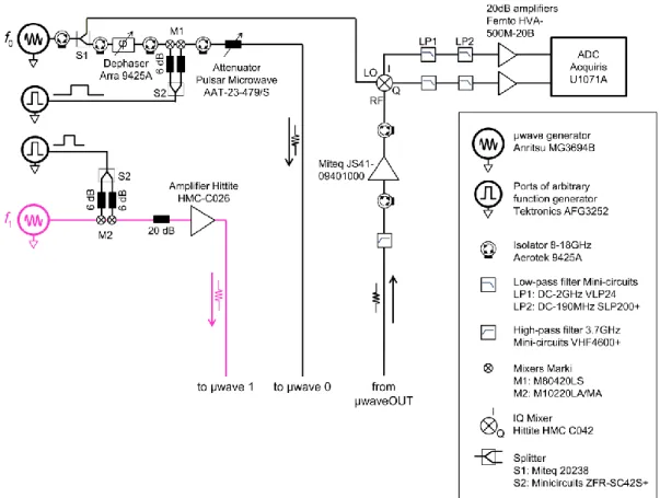
Fig. S1: Microwave setup at room temperature. There are two lines to inject driving (“µwave1”) and measurement (“µwave0”) pulses, and one line (“µwaveOUT”) that carries the reflected signal at the measurement frequency. Microwave pulses are shaped by mixing continuous waves from the microwave sources with DC pulses from a 2-port arbitrary function generator. The latter and the acquisition board (ADC) are synchronized and triggered by an arbitrary waveform generator (Agilent AWG 33250, not represented). In order to improve the ON-OFF contrast of the microwave pulses, a second AWG (not represented) is used to pulse the
f
1 microwave source itself.18
Fig. S2: Low temperature wiring. The three lines “µwave1”, “µwave0” and “µwaveOUT” correspond to those of Fig. S1. The sample is enclosed in four shields: the inner one is made out of epoxy loaded with brass and carbon powder, the 2nd one out of aluminum, the 3rd one out of Cryoperm, the 4th one out of copper. The sample and the shields are thermally anchored to the mixing chamber of base temperature 30 mK. The cryogenic microwave amplifier is a commercial HEMT (CITCRYO1-12A-1 from Caltech) with nominal gain 32 dB and noise temperature 7 K at 10 GHz. A DC magnetic field is applied perpendicular to the chip using a small superconducting coil placed a few mm above the aluminum loop containing the atomic contact. Biasing is performed using a voltage source (iTest BILT BE2102) in series with a 200 k resistor. Filtering is provided partly by a 1 resistor placed at 0.7 K in parallel with the coil.
19
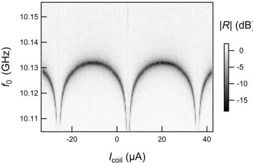
Fig. S3: Periodicity of VNA measurements with flux. Modulus R of reflected signal as a function of the current Icoil through the superconducting coil for a contact with several channels. The period allows calibrating the current associated with one flux quantum in the aluminum loop, i.e. with a 2 change in the phase across the contact. The currents at which the resonance frequency (dark) presents broad maxima correspond to 0 modulo 2 .
20
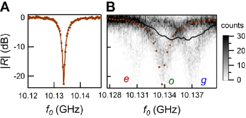
Fig. S4: Vector network analyser (VNA) measurements of the resonator for the contact with 0.99217described in the manuscript. (A) Amplitude R of reflexion coefficient as a function of the probe frequency
f
0 when the resonator and the Andreev doublet are far detuned ( 0.9 , fA 15.9GHz), corresponding to a vertical cut on the left edge of Fig. 3B. Symbols: measurement acquired at low power, corresponding to n 0.1 photons in the resonator and a 10 Hz acquisition bandwidth. Solid line: fit using1 2 2 1 R 1 / 4 q Qx q with x f0/ fR1 and / ext
q Q Q. The dip signals the resonance frequency
f
R10.134GHz
, with total quality factor Q2200 and external quality factorQ
ext
4800
associated with the coupling capacitor. (B) R measured at . Black curve is taken at low power (0.1
n photons in resonator) and a 10 Hz acquisition bandwidth (corresponds to a cut in the middle of Fig. 3B). Image in the background is a two-dimensional histogram of 32000 data points taken in a single frequency sweep with a 600 kHz
bandwidth, and a larger power (n 40 at resonance). We observe three replicas of the resonance as measured at 0.9 (brown symbols, same data as (A)). The central one corresponds to odd state o , the rightmost to g and the leftmost (barely visible) to e .
21
Fig. S5: Time-resolved response of the resonator to a 2 µs-long probe pulse. Black: 0.1 GHz-detuned pulse: complete reflection. Red: pulse at resonance frequency. After a loading time 2 / of the cavity, wave exiting the cavity interferes destructively with reflected wave. The negative signal after t=2µs corresponds to photons exiting the cavity after the end of the pulse. Blue: exponential fit, with decay time
2 / 69 ns. Total quality factor of the cavity is Q / 2200 in agreement with fit of cavity resonance (see Fig. S4A).
22
Fig. S6: Data for an atomic contact different from the one in the main text. (A) Pulsed two-tone spectroscopy: color coded amplitude A of one quadrature of reflected signal as a function of and
f
1. Dashed black line: theoretical fit of Andreev transition frequencyf
A
2
E
A/
h
with 0.99806. Two-photon processes (dash-dotted line labelled fA/2) are observed because a higher excitation power than the one used for Fig. 3. (B) Single-tone continuous-wave spectroscopy using a vector network analyzer (n 0.1): resonator reflection amplitude R as a function of andf
0. Red dashed curves: fits of the anti-crossings using g( ) / 2 72 MHz. Compared to Fig. 3, this data was taken on a different cool-down of the sample, and the bare resonator frequency was 10.121 GHz. (C) Density plots of I, Q quadratures at illustrate single-shot resolution of the quantum state of the dot. Top panel: no drive atf
1. Bottom panel: pulse results in a population transfer from g to e .23
Fig. S7: Data for same contact as in Fig. S6, to be compared with Fig. 4. (A) Spectroscopy. (B) relaxation after a -pulse. (C) Rabi oscillations (note break and change in scale of x-axis). (D) Ramsey fringes with 50 MHz detuning. (E) Hahn echo.
24
Fig. S8: Data for contact with channel transmission 0.99647, to be compared with Fig. 4. (A) Spectroscopy. (B) relaxation after a -pulse. (C) Ramsey fringes with 95 MHz detuning. (D) Hahn echo.
25
Fig. S9 (snapshot from Movie S1): (Left) Density plot of I and Q quadratures for a 380 ns-long Rabi pulse. (Right) Evolution of the populations of states g (blue), e (red) and o (green) for Rabi pulse lengths up to 380 ns.
Movie S1: (animated Gif image, available on the Science website) Rabi oscillations seen in the I,Q plane, and corresponding evolution of the populations: the populations of the ground state ( g ) and the excited state ( e ) swap, whereas the population of the odd state ( o ) remains constant. Data correspond to Fig. 3C of paper, with a rotation in the I,Q plane.