The faint young Sun problem revisited with a 3-D climate–carbon model – Part 1

HAL Id: hal-02902788

https://hal.archives-ouvertes.fr/hal-02902788

Submitted on 21 Jul 2020

HAL is a multi-disciplinary open access

archive for the deposit and dissemination of

sci-entific research documents, whether they are

pub-lished or not. The documents may come from

teaching and research institutions in France or

abroad, or from public or private research centers.

L’archive ouverte pluridisciplinaire HAL, est

destinée au dépôt et à la diffusion de documents

scientifiques de niveau recherche, publiés ou non,

émanant des établissements d’enseignement et de

recherche français ou étrangers, des laboratoires

publics ou privés.

The faint young Sun problem revisited with a 3-D

climate–carbon model – Part 1

G. Le Hir, Y. Teitler, F. Fluteau, Yannick Donnadieu, P. Philippot

To cite this version:

G. Le Hir, Y. Teitler, F. Fluteau, Yannick Donnadieu, P. Philippot. The faint young Sun problem

revisited with a 3-D climate–carbon model – Part 1. Climate of the Past, European Geosciences Union

(EGU), 2014, 10 (2), pp.697-713. �10.5194/cp-10-697-2014�. �hal-02902788�

www.clim-past.net/10/697/2014/ doi:10.5194/cp-10-697-2014

© Author(s) 2014. CC Attribution 3.0 License.

Climate

of the Past

The faint young Sun problem revisited with a 3-D climate–carbon

model – Part 1

G. Le Hir1, Y. Teitler1,*, F. Fluteau1, Y. Donnadieu2, and P. Philippot1

1_{IPGP, Institut de Physique du Globe de Paris, Sorbonne Paris cité, Université Paris Diderot, UMR7154, 75005, France} 2_{LSCE, CNRS-CEA-UVSQ, 91191 Gif-sur-Yvette, France}

*_{now at: Centre for Exploration Targeting, University of Western Australia, Crawley, Australia} Correspondence to: G. Le Hir (lehir@ipgp.fr)

Received: 6 February 2013 – Published in Clim. Past Discuss.: 22 March 2013 Revised: 17 February 2014 – Accepted: 18 February 2014 – Published: 3 April 2014

Abstract. During the Archaean, the Sun’s luminosity was 18

to 25 % lower than the present day. One-dimensional radia-tive convecradia-tive models (RCM) generally infer that high con-centrations of greenhouse gases (CO2, CH4) are required to

prevent the early Earth’s surface temperature from dropping below the freezing point of liquid water and satisfying the faint young Sun paradox (FYSP, an Earth temperature at least as warm as today). Using a one-dimensional (1-D) model, it was proposed in 2010 that the association of a reduced albedo and less reflective clouds may have been responsi-ble for the maintenance of a warm climate during the Ar-chaean without requiring high concentrations of atmospheric CO2 (pCO2). More recently, 3-D climate simulations have

been performed using atmospheric general circulation mod-els (AGCM) and Earth system modmod-els of intermediate com-plexity (EMIC). These studies were able to solve the FYSP through a large range of carbon dioxide concentrations, from 0.6 bar with an EMIC to several millibars with AGCMs. To better understand this wide range in pCO2, we investigated

the early Earth climate using an atmospheric GCM coupled to a slab ocean. Our simulations include the ice-albedo feed-back and specific Archaean climatic factors such as a faster Earth rotation rate, high atmospheric concentrations of CO2

and/or CH4, a reduced continental surface, a saltier ocean,

and different cloudiness. We estimated full glaciation thresh-olds for the early Archaean and quantified positive radiative forcing required to solve the FYSP. We also demonstrated why RCM and EMIC tend to overestimate greenhouse gas concentrations required to avoid full glaciations or solve the FYSP. Carbon cycle–climate interplays and conditions for sustaining pCO2will be discussed in a companion paper.

1 Introduction

Sagan and Mullen (1972) argued from solar models that, in the early Archaean, the young Sun’s luminosity was 25 % lower compared to now. According to climate models, the weakness of the young Sun’s brightness would have implied that Earth’s surface temperature was well below the freezing point of water during the first two billion years of its history. A completely frozen Earth, however, conflicts with evidence of the presence of liquid water at the surface and life develop-ment during the Archaean. More intriguingly, geological evi-dence suggests that the Archaean climate was similar or even warmer than the present-day climate. Greenhouse gases, and more specifically carbon dioxide, were soon put forward as good candidates for solving this issue known as the “faint young Sun paradox” (FYSP; see Feulner, 2012 for a detailed review). Using a vertical one-dimensional radiative convec-tive climate model (RCM), Kasting (1984, 2010) calculated that an atmospheric carbon dioxide partial pressure (pCO2)

of 0.3 bar or ∼ 1000 times the preindustrial atmospheric level (PAL) (i.e. 0.28 mbar or 280 ppm) was needed to maintain a mean global surface temperature of 15◦C for a Sun 75 % dimmer than today.

In parallel with the modelling approach, atmospheric carbon dioxide concentration was semi-quantitatively esti-mated from Archaean palaeosols. Considering the absence of siderite in 2.8 Ga-old palaeosols, Rye et al. (1995) sug-gested from thermodynamical modelling that the pCO2had

not exceeded ∼ 0.04 bar (or ∼ 130 PAL) during the Late Ar-chaean. Questioning the relevance of the Rye et al. (1995) approach, Sheldon (2006) conducted mass-balance calcula-tions of weathering in several Archaean to Palaeoproterozoic

698 G. Le Hir et al.: The faint young Sun problem

palaeosols and proposed that the pCO2 fluctuated from

3 mbar to 26 mbar (i.e. 11 to 93 PAL) from 2.2 to 1.0 Ga. More recently, Driese et al. (2011), using palaeoweather-ing indicators, suggested moderate CO2 partial pressures

of about 10 mbar at 2.7 Ga ago. Given the composition of iron-rich minerals found in Archaean banded iron forma-tions (BIFs), Rosing et al. (2010) argued that the coexis-tence of magnetite (i.e. Fe3O4, a moderately oxidised

min-eral) and siderite (i.e. FeCO3, a reduced mineral) in BIF was

dependent on the atmospheric level in di-hydrogen (pH2).

Di-hydrogen (H2) is a nutrient for methanogenic bacteria,

and biological constraints impose a minimum pH2. Using

this constraint, Rosing et al. (2010) defined an upper limit for pCO2 of about 0.9 mbar (900 ppmv or 3.2 PAL). Such

a low pCO2 has been the core of vivid debate among

spe-cialists, notably because BIFs are formed in marine envi-ronments far from thermodynamic equilibrium with the at-mosphere and therefore are poor proxies of the early Earth atmosphere composition (Dauphas and Kasting, 2011; Rein-hard and Planavsky, 2011).

Given the difficulties in estimating the partial pressure of atmospheric greenhouse gases on the primitive Earth, other mechanisms influencing climate such as changes in cloud properties have been explored. The mean forcing of clouds results from two opposite effects (Pierrehumbert, 2010). Clouds are highly reflective in the spectrum of visible solar radiation (shortwave radiation) and highly absorbent in the spectrum of thermal terrestrial radiation (longwave radiation). This leads to two well-known opposite effects; the shortwave reflection effect contributing to the planetary albedo and the longwave absorption effect contributing to the greenhouse. These mechanisms are related to the cloud type, the greenhouse effect being stronger than the albedo effect in the case of cirrus clouds, which are quite trans-parent at visible wavelengths but good absorbers of ther-mal terrestrial radiation. Using a one-dimensional radiative model, Goldblatt and Zahnle (2011b) estimated that in or-der to compensate for a weak Sun, Earth must have been en-tirely cloud-covered with poorly reflective (i.e. absence of stratus) but 3.5 times thicker clouds than today. In the ab-sence of a mechanism able to change cloud properties in such proportions, the authors concluded that this scenario was highly unlikely. Goldblatt and Zahnle (2011b) also chal-lenged Rosing et al.’s (2010) hypothesis that thinner clouds, caused by sparse cloud condensation nuclei (CCN), could have acted as an alternative to atmospheric greenhouse gases to warm up the early Earth’s surface. In the present-day atmo-sphere, abundant CCN permit the formation of small liquid water droplets, leading to optically dense and highly reflec-tive clouds because of their direct scattering effect (Charlson et al., 1987). During the Archaean, the concentration of CCN would have been about 10 to 20 % of its natural present-day level due to lower organic and inorganic sources. As a consequence, fewer droplets, but of larger size, would have formed optically thin clouds characterised by a low scattering

of shortwave radiations and shorter lifetime. This hypothesis had been quantified with RCM simulations (Rosing et al., 2010). However, using a more realistic treatment of clouds, Goldblatt and Zahnle (2011b) demonstrated that the radia-tive forcing due to such changes in cloud properties has been overestimated.

To go one step further in the understanding of the FYSP, Kienert et al. (2012) conducted the first 3-D climate mod-elling of the Archaean climate using the EMIC (Earth sys-tem models of intermediate complexity) CLIMBER, which consists in an ocean general circulation model coupled with a simplified, low-resolution atmosphere. Using Archaean boundary conditions including a reduced incoming solar ra-diation, a faster Earth rotation and a reduced continental sur-face, CLIMBER simulates a present-day climate for a car-bon dioxide partial pressure fixed at 0.6 bar. The authors ex-plained their results by the ice-albedo feedback, which is en-hanced during the Archaean due to a faster Earth rotation rate. This result contrasts with conclusions obtained by Jenk-ins (1993b) and JenkJenk-ins et al. (1993) with CCMAO (CC-MAO was the version of the NCAR model at the begin-ning of the 90s, an atmospheric GCM coupled to a swamp ocean without heat capacity), where a faster rotation rate would have induced a warmer climate. The recent mod-elling of Archaean climate by Charney et al. (2013) using LMDz (an atmospheric GCM coupled to a slab ocean de-veloped by Laboratoire de Météorologie Dynamique) chal-lenged the CLIMBER results (Kienert et al., 2012, 2013) and revealed a very limited impact of the faster Earth ro-tation. However, LMDz results suggest that, for 3.8 Ga-old conditions, 100 mbar of carbon dioxide and 2 mbar of CH4

are required to maintain an Earth climate as warm as today. Similar results are predicted for the Late Archaean (2.7 Ga), with the atmospheric GCM coupled to a slab ocean CAM3 (Wolf and Toon, 2013), where a combination of 20 mbar of CO2and 1 mbar of CH4 is required to yield a global mean

surface temperature near that of the present day.

To understand why AGCMs (Charney et al., 2013; Wolf and Toon, 2013; Kunze et al., 2014), EMIC (Kienert et al., 2012, 2013) and RCMs (Rosing et al., 2010; Kasting, 1984) differ in simulating the early Earth climate, we investigated the Precambrian climate using an atmospheric general circu-lation model coupled to a slab ocean FOAM. The paper is organised as follows. First, we estimate the radiative deficit required for the onset of a pan-glaciation. We run experi-ments ranging from 3.5 to 1 Ga to explore the impacts of Ar-chaean boundary conditions (solar constant, palaeogeogra-phy, amount of emerged continental surface, and cloud prop-erties). Second, we investigate the faint young Sun problem by performing additional sets of simulations where the ef-fects of greenhouse gases (CO2 and CH4), saltier oceans,

faster Earth rotation or sea ice albedo are tested. Finally, we compare our results with the above-mentioned studies to explore the causes of observed differences among RCMs,

10

10

10

10

10

10

-∆F trop [W/m

]

-20

20

-40

40

0

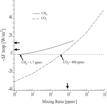
Fig. 1. Net long-wave fluxes computed for CO2and CH4with the

FOAM radiative code (NCAR ccm3) (the total atmospheric is held constant, 1 bar). Thick arrows indicate the radiative forcing

corre-sponding to 0.9 mbar of CO2and CH4. Using the present-day

at-mosphere as a reference, the change in net flux at the tropopause

(1Ftrop) is 19 W m−2, which reduces to 6 and 13 W m−2 for

0.9 mbar of CO2and CH4, respectively.

EMIC and AGCMs, and discuss how these models differ in representing the ice-albedo feedback mechanism.

2 Model description and simulation specifications 2.1 Model description

Climate simulations were run with the atmospheric general circulation climate model (AGCM) FOAM 1.5. The atmo-spheric component of FOAM is a parallelised version of NCAR’s Community Climate Model 2 (CCM2) with the upgraded radiative and hydrologic physics incorporated in CCM3 v. 3.2 (Jacob, 1997). All simulations were performed with an R15 spectral resolution (4.5◦×7.5◦) and 18 verti-cal levels. The radiative code (extracted from NCAR CCM3) has already shown its validity in atmospheres highly enriched in CO2 (Pierrehumbert, 2004; Le Hir et al., 2010). The

in-frared absorption has been computed (Fig. 1) to replace CO2

-CH4 conversion proposed by Rosing et al. (2010). Under

an enriched CH4atmosphere, no significant differences are

observed compared to prior estimates (Kiehl and Dickin-son, 1987; Halevy et al., 2009). FOAM integrates the CCM3 version of cloud water parameterisation. As in the CCM3, cloud optical properties and liquid water droplet clouds used the Slingo (1989) parameterisation, where the liquid water droplet clouds (Cloud Water Path or CWP) is determined by

integrating the liquid water concentration (qclw):

CWP =

Z

qclw.dz where qclw=qclw0e(−z/Hclw) (1)

z being the altitude, qclw0 an empirical constant equals to

0.21 g m−3 _{and H}

clw the scale height representing the total

precipitable water column, which is dependent of the precip-itable water (qtot). This last equation implies an exponential

decay for in-cloud water concentration,

Hclw=700 ln(1 + qtot) (2)

with qtot being computed by integrating the specific

humid-ity Q (in kg kg−1)over dp, p being the pressure and g the gravitational acceleration (9.8 m s−2):

q_tot = 1/g ∗

Z

Qdp. (3)

FOAM is used in mixed-layer mode, meaning the atmo-spheric model is linked to a 50 m mixed-layer ocean with heat transport parameterised through diffusion. The diffusive rate of the slab ocean (Qflux)is derived from the net surface

fluxes and fixed to represent sea ice-covered seas based on estimates of the present-day sea ice mass budget. The sea ice module uses the thermodynamics of NCARs to compute ice fraction (growth and melting), snow cover, and penetrating radiation, and includes a Semtner model to calculate the sea ice temperature. The sea ice module does not treat sea ice dynamics, a lack which may slow the sea ice flow and un-derestimate the sea ice cover (Voigt and Abbot, 2012). Sea ice albedo is fixed at 0.7 (visible spectrum) and 0.5 (near-infrared spectrum).

2.2 Boundary conditions and experimental design

In this section, we describe boundary conditions used to ex-plore the effects of solar constants, palaeogeography (amount of continental surface), and cloud properties from 3.5 to 1 Ga ago. Sets of simulations are summarised in Table 1.

2.2.1 Solar irradiance and palaeogeographies

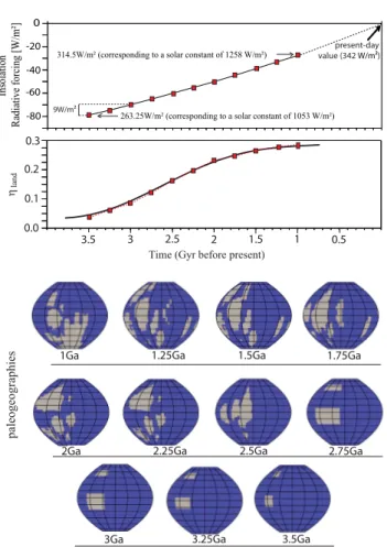
Following Gough’s formula (1981), the solar constant has been increased by 19 %, from 3.5 Ga (1053 W m−2)to 1 Ga (1258 W m−2)(Fig. 2a). Orbital parameters were set at their present-day values (orbital eccentricity: 0.016724, obliquity: 23.4463, vernal equinox latitude of perihelion: 77.9610) in all experiments. We varied the continental surface in re-sponse to the crustal growth and emergence, a process which affected the mean surface albedo (αocean=0.06, αbare˙soil=

0.32). Different scenarios ranging from a progressive for-mation to a quasi-instantaneous forfor-mation of all continental crust have been proposed (see Lowe and Tice, 2007 for a detailed review). Here we considered a gradual continental growth (Fig. 2b), consistent with the changes of87Sr/86Sr

700 G. Le Hir et al.: The faint young Sun problem

Table 1. Simulations performed in the Sect. 3 (1Ftropis held constant and equals to +19 W m−2).

set of Boundary conditions LOD Droplet seawater

simulations Paleogeography Solar constant (hours) size(µm) freezing point

modern clouds 3.5-1Ga (Fig. 2b) 3.5-1Ga (Fig. 2a) 24 5–10 −1.8◦C

no clouds “ “ 24 / “

Large droplet clouds “ “ 24 20 “

land

η

3.5

Time (Gyr before present)

Insolation Radiative forcing [W/m²] 263.25W/m² (corresponding to a solar constant of 1053 W/m²)

0

-20 -40 -60

314.5W/m² (corresponding to a solar constant of 1258 W/m²)

9W/m² 0.3 0.2 0.0 0.1 3 2.5 2 1.5 1 0.5 -80 paleogeographies

1Ga 1.25Ga 1.5Ga

1Ga 1.25Ga 1.5Ga 1.75Ga

2Ga 2.25Ga 2.5Ga 2.75Ga

3Ga 3.25Ga 3.5Ga

present-day value (342 W/m²)

Fig. 2. Boundary conditions for solar constant (upper part) and

con-tinental growth (lower part). ηlandis the emerged surface/Earth

sur-face ratio (the present-day sursur-face is 146 × 106km2or 29 % of the

Earth’s surface). Each red square represents the boundary condi-tions used in our sets of simulacondi-tions.

(Godderis and Veizer, 2000) and δ34S throughout the Ar-chaean and early Proterozoic. Accordingly, the surface of the emerged continents increased from 4 % at 3.5 Ga to 27.5 % at 1 Ga. Palaeogeographies were reconstructed based on paleo-magnetic data from 1 to 2.5 Ga (Pesonen et al., 2003). 3.5 to 2.75 Ga plate reconstructions being poorly constrained, continents were assumed to be located at low and mid lati-tudes. The elevation of land points was fixed at 200 m in all experiments.

2.2.2 Radiative forcing by greenhouse gases and ozone amounts

To set up boundary conditions correctly, we estimated the greenhouse radiative forcing provided by the combination of 0.9 mbar of CO2 and CH4 (i.e. CO2 and CH4

concen-trations used by Rosing et al. (2010) and also tested by Charney et al. (2013)), rather than directly use pCO2 and

pCH4 as boundary conditions. This was motivated because

the assumption of such a low CO2/high CH4is likely

incor-rect (Dauphas and Kasting, 2011; Reinhard and Planavsky, 2011). Moreover, Rosing et al. (2010) ignored the organic haze formation ([CH4]/[CO2] > 0.2 (Haqq-Misra et al.,

2008)). Since it makes little difference whether radiative forcing is controlled by CO2or CH4(Hansen et al., 1997),

this approach avoids doubtful assumptions about the Ar-chaean/Proterozoic atmosphere composition. Hence, using the present-day atmosphere as a reference, the change in net radiative flux at the tropopause (1Ftrop, Fig. 1) equals

19 W m−2 (1Ftrop=6 and 13 W m−2 for 0.9 mbar of CO2

and CH4, respectively).

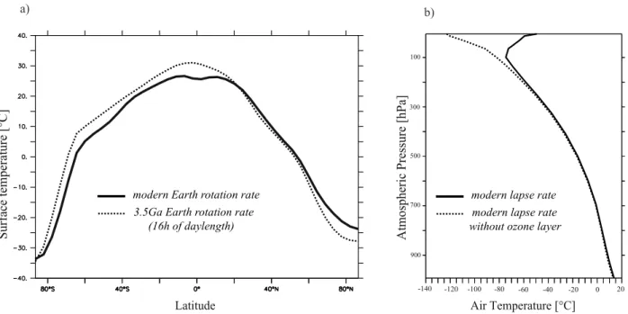
In addition, due to the low oxygen content of the Archean atmosphere imposed by sulfur mass independent fraction-ation (S-MIF) of sedimentary sulfides and sulfates (10−5 Present Atmospheric Level, PAL, Farquhar et al., 2001; Pavlov et al., 2000), the stratospheric ozone layer was re-moved in all experiments prior to 2.25 Ga and constrained to the present-day value in other experiments. The absence of an ozone layer precluded the formation of a stratospheric temperature inversion and resulted in a 40 km-thick atmo-sphere without temperature stratification (corresponding to the topmost atmospheric grid points in the AGCM). The global mean lapse rate from the surface to the 200 hPa level was not significantly affected by the absence of the ozone layer, and only a slight mean global cooling (0.7◦C) was simulated at the Earth’s surface (Appendix Fig. A1). Induced cooling of surface temperature (1 to 2◦C) associated with the removal of the ozone layer is in good agreement with previ-ous studies (Kasting, 1984; Kiehl and Dickinson, 1987; Wolf and Toon, 2013; Kunze et al., 2014).

2.2.3 Experimental design and assumptions for clouds

We performed sets of numerical experiments ranging from 3.5 to 1 Ga ago with a 0.25 Ga time increment. To avoid any effect of initial boundaries, simulations were initiated with warm conditions (present-day as starting point) and driven toward colder conditions (step-like decrease in the Sun’s brightness). Each run lasted several tens of years un-til a steady state was reached for a decade or more. Climatic variables are averaged over the last decade.

To test the radiative impact of clouds, we considered three scenarios involving modern clouds, no cloud at all (cloud fraction fixed to 0), and clouds with large droplets (Table 1). A change in cloud droplet size affects scattering and there-fore the cloud albedo (Pierrehumbert, 2010). For the parame-terisation of Slingo (1989) implemented in FOAM, the cloud optical properties (OPclds)for short-wave radiations were

de-fined as

OPclds=CWP[a + b/re], (4)

where a and b are the cloud radiative coefficients (different for ice or liquid water clouds), CWP the cloud water path (g kg−1) and re the effective droplet radius (droplet radius

affected by its distribution).

In FOAM, liquid cloud droplet radii of modern clouds vary from 5 to 10 µm over landmasses and are fixed at 10 µm over oceans. This distinction is made to account for enhanced cloud drop nucleation that can occur over CCN-rich land areas. On the modern Earth, non-anthropogenic production of CCN is essentially related to soil dust formation, vol-canic sulfate aerosols and dimethylsulfide (DMS) produced by planktonic eukaryotic algae (Charlson et al., 1987; An-dreae and Rosenfield, 2008). In the absence of planktonic al-gae during the Archaean, the scarcity of emerged terrestrial surfaces and subaerial volcanism were considered as the pos-sible, yet speculative, causes for the low CCN availability in the early Earth atmosphere (Rosing et al., 2010). To quantify the influence of large liquid droplets on climate, we ran a set of experiments in which we used the mean radius of liquid droplets of 20 µm1 used by Rosing et al. (2010) over both the oceans and continents. Cloud droplets exceeding 15 µm being rarely observed (Bréon et al., 2002), this set of simula-tions should be regarded as an end member. Although large liquid water droplets of 20 µm diameter are expected to re-duce cloud albedo (scattering effect), they also tend to rain out more rapidly (Boucher et al., 1995). According to the relationship established by Kump and Pollard (2008), the en-hancement of cloud-to-precipitation rate varies as

cloud-to-precipitation rate = (re/reo)n, (5)

where rerepresents the new effective radius (20 µm), reothe

modern effective radius (assumed to be 10 µm, as oceans

1_{The effective radius of 20 µm used by Rosing et al. (2010) was}

finally revised to 17 µm (Goldblatt and Zahnle, 2011a).

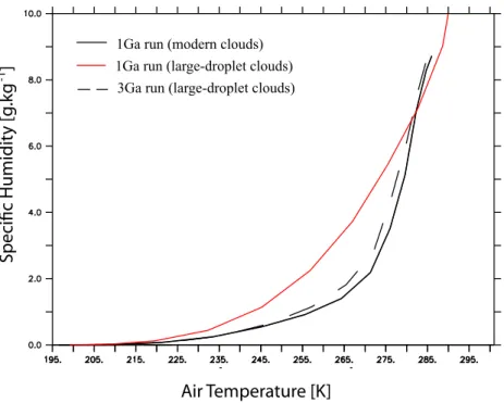
cover a large fraction of the Earth’s surface), and n the pa-rameter of enhanced rain-out (here n = 3). The literature fea-tures a wide range of values for the enhanced rain-out pa-rameter; here we used an intermediate value suggesting a mid-strength feedback between 1 and 5.37 (Goldblatt and Zahnle, 2011b; Penner et al., 2006; Charney et al., 2013). As the cloud lifetime cannot be changed in the absence of a cloud microphysics module, we increased the precipitable water by 8 to represent the enhanced rain-out. Albeit specu-lative (see Sect. 2.1), we showed that CWP fluctuations are only governed by the air moisture (Appendix Fig. A2).

3 Results: estimating pan-glaciation thresholds

Figure 3 shows the radiative deficit required to induce a pan-glaciation, the global mean surface temperature and the mean planetary albedo. It is worth emphasising that the results presented here are not representative of climate evolution over the Precambrian era because only part of the boundary conditions used are realistic (solar luminosity, palaeogeogra-phy, fraction of emerged land). Other boundary conditions including the greenhouse gas radiative forcing (1Ftrop=

+19 W m−2) are unrealistic. However, these were imple-mented in our model to allow comparison with previous sim-ulations (Charney et al., 2013; Rosing et al., 2010) and to determine the radiative forcing threshold values required for the onset of pan-glaciations. The experiments (Exp) are la-belled from 3.5 to 1 Ga according to the boundary conditions used.

3.1 Influence of the solar constant

Figure 3b (blue curve) represents the global mean surface temperature (Ts) simulated using the present-day cloud pa-rameterisation. Ts is as low as −75◦C in Exp(3.5 Ga) and increases linearly up to −65◦C in Exp(2.5 Ga). The plane-tary albedo always exceeds 0.65 (Fig. 3c, blue curve) when the Earth is ice covered. An abrupt change, expressed by a shift of both temperature and albedo, is observed between Exp(2.5 Ga) and Exp(2.25 Ga). In Exp(2.25 Ga), Ts reaches

−20◦C and the albedo drops to 0.45. This corresponds to a partially frozen Earth where sea ice spreads up to 30◦ latitude in both hemispheres. Between Exp(2.25 Ga) and Exp(1.75 Ga), a slight global warming of about 5◦C is ob-served, followed by a marked change of some 24◦_{C between}

Exp(1.75 Ga) and Exp(1.25 Ga), and a final slight warming of 4◦_{C between Exp(1.25 Ga) and Exp(1 Ga).}

From these experiments, three climate states can be defined; a snowball Earth between Exp(3.5 Ga) and Exp(2.5 Ga), a partially frozen Earth between Exp(1.75 Ga) and Exp(2.25 Ga), and a weakly frozen Earth between Exp(1 Ga) and Exp(1.25 Ga). Although the solar brightness increased sub-linearly between 3.5 and 1 Ga, the global mean surface temperature changed dramatically during this time

702 G. Le Hir et al.: The faint young Sun problem

Time (Gyr before present)

Tsurface [ºC] (annual mean) Planetary albedo Rosing et al. (2010) 0.15 Rosing et al. (2010) (1Gyr) (3Gyr) (3.5Gyr) 4 3.5 3 2.5 2 1.5 1 0.5 0. 2 3 1 2 3 1

Sea ice extent (annual mean)

a) b) c) d) RCM (no cld runs) -40 -50 -60 -70 -80 Sun Radiative Forcing

Radiative forcing [W/m²] pan-glaciation threshold (FOAM runs **) pan-glaciation threshold (FOAM runs *)

RCM no clds runs, 0°C line

Figure 3:

3D climate simulations from 3.5 to 1 Ga with a greenhouse radiative forcing by CO and CH fixed to 19W.m

(∆Ftrop; see figure 1). a) Radiative deficit required for the onset of a pan-glaciation with RCM (no cloud runs, surface

albedo fixed to 0.264), FOAM runs (* modern clouds and cloud-free runs and ** large-droplet clouds (20μm)). Grey lines represent uncertainties related to temporal resolution (0.25Ga). b) Evolution of surface temperature versus time assuming increasing irradiance and linear continental growth (see figure 2). Grey line is from Rosing et al. (2010). Blue and red curves were obtained using liquid droplets sizes of 5 to 10μm (modern clouds) and 20μm (clouds with large droplets), respectively. Green squares represent the cloud-free scenario. c) Evolution of planetary albedo versus time (αocean 0.06, αrocky desert continents 0.32, αseaice 0.6, αsnow 0.8). d) Red stars represent sea ice extent (white) predicted

with runs performed with large (20μm) droplets (figures 3b,c show corresponding temperature / albedo).

-2

2 4

Fig. 3. 3-D climate simulations from 3.5 to 1 Ga with a

green-house radiative forcing by CO2 and CH4 fixed to 19 W m−2

(1Ftrop; see Fig. 1). (a) Radiative deficit required for the onset

of a pan-glaciation with RCM (no cloud runs, surface albedo fixed to 0.264), FOAM runs (* modern clouds and cloud-free runs and ** large-droplet clouds (20 µm)). Grey lines represent uncertain-ties related to temporal resolution (0.25 Ga). (b) Evolution of sur-face temperature versus time assuming increasing irradiance and linear continental growth (see Fig. 2). Grey line is from Rosing et al. (2010). Blue and red curves were obtained using liquid droplet sizes of 5 to 10 µm (modern clouds) and 20 µm (clouds with large droplets), respectively. Green squares represent the cloud-free

sce-nario. (c) Evolution of planetary albedo versus time (αocean 0.06,

αrocky desert continents0.32, αseaice0.5, αsnow0.8). (d) Red stars

rep-resent sea ice extent (white) predicted with runs performed with large (20 µm) droplets (Fig. 3b, c shows the corresponding temper-ature/albedo).

period (Fig. 3b). Between 1 and 1.25 Ga, the solar brightness is high enough to restrict the sea ice capping to the high lati-tudes (∼ 60◦_{) and to bring the equator-pole surface}

tempera-ture gradient to the present-day level. Between Exp(1.25 Ga) and Exp(1.75 Ga), sea ice spreads towards the equator up to 30◦of latitude due to the reduced incoming solar radiation. Between Exp(1.75 Ga) and Exp(2.25 Ga), the sea ice max-imum extent remains located in the vicinity of the tropics. This is due to a latitudinal gradient of temperature two times higher than in the Exp(1 Ga), which arises from a strong meridional energy transport by the atmosphere and oceans. For a solar constant lower than 1148 W m−2 (2.25 Ga), the solar brightness is low enough to drive climate towards snow-ball Earth conditions. Hence, for a fixed greenhouse-gas con-centration of 1Ftrop= +19 W m−2, the solar constant

evolu-tion and its interplay with the ice-albedo feedback appear as the predominant factor governing the Earth’s climate. This contrast with the RCM results (Fig. 3a) where the albedo is held constant at 0.264 (Goldblatt and Zahnle, 2011b) due to the absence of the ice-albedo feedback.

3.2 Influence of continental surfaces

A lower surface albedo due to a reduced continental area (αbare soil=0.32, αocean=0.06) has been suggested as a

solution to the FYSP (Schatten and Endel, 1982; Ros-ing et al., 2010; but see Walker et al., 1982 and Gol-batt and Zanhle, 2011, for a controversy). No-cloud exper-iments show that the planetary albedo, which corresponds to the surface albedo, fluctuates with the growth of sea ice (Fig. 3b, green curve). Using the amount of energy reach-ing the Earth (expressed by F = S/4(1-α), with 1α = 0.10 and S = 1148 W m−2_{), we estimated the radiative forcing}

in-duced by the ice-albedo feedback to −29 W m−2(cooling ef-fect) between 1 and 2.25 Ga. This calculation shows that a slight change in the sea ice surface (αsea-ice=0.6) can

eas-ily overcome the influence of a smaller continental area on the surface albedo (αbare soil=0.32, αocean=0.06). These

re-sults demonstrate that the surface albedo is mainly governed by the sea ice extension, the growth of continental surfaces being a second-order factor. This conclusion is to challenged when the climate–carbon cycle feedbacks will be consid-ered (Walker et al., 1981; Godderis and Veizer, 2000) (see companion paper).

3.3 Influence of clouds

Cloud experiments performed at 1 Ga show that the cloud radiative forcing is equal to −10 and −20 W m−2 at high and mid-latitudes, respectively (Fig. 4b). Accordingly, the absence of clouds seems to limit the sea ice spreading at high latitudes and to prevent the increase in the planetary albedo (Fig. 3c). This mechanism can explain why cloud-free experiments result in a warmer climate than those using modern clouds (Fig. 3b, green curve). Surprisingly, the shift

CRF [W/m²]

0 40S

80S 40N 80N

CRF [W/m²]

Time (Ga before present)

4 3.5 3 2.5 2 1.5 1 0.5 0. Sw/Lw CRF [W/m²] 80 60 40 20 -60 -40 -20 0 40 20 -20 0

LW (large droplets clouds)

LW (modern clouds)

SW (large droplets clouds) SW (modern clouds) 0 40S 80S 40N 80N Latitudes a) b) c) Latitudes

large droplets clouds

modern clouds

Fig. 4. (a) Net cloud radiative forcing (CRF, unit W m−2)

ver-sus time. Blue squares represent runs with modern clouds. Large-droplet clouds (red squares) result in a positive forcing because the effect of infrared trapping overcomes that of scattering. (b) CRF as a function of latitude for simulations performed at 1 Ga. The black line represents large-droplet clouds and the dashed line the mod-ern cloud parameterisation. (c) Simulations performed using 1 Ga boundary conditions. Dashed lines represent long-wave (LW) bud-get of clouds (greenhouse effect), continuous lines their short-wave budget (albedo effect).

from a snowball state toward a partially ice-free Earth oc-curs between 2.5 and 2.25 Ga in both types of experiments. However, this apparent synchronicity is due to the relatively long duration increment of 250 Ma used between experi-ments. Since the incoming solar energy varies by as much as 5 W m−2_{between 2.5 and 2.25 Ga (Fig. 2), it is not possible}

to evaluate with precision when the pan-glaciation occurs. In addition, it cannot be excluded that in a cold climate environ-ment, the cloud scheme of FOAM underestimates the cloud radiative forcing (Abbot et al., 2012).

3.4 Effects of the cloud droplet size

The use of large liquid droplets (20 µm) increases the global mean surface temperature by about 20 to 35◦C compared to present-day droplet sizes (Fig. 3, red curves). In the large-droplet experiments, the shift towards snowball state occurs between 3 and 3.25 Ga with a mean global surface

temper-ature of 13◦_{C. In contrast, modern clouds experiments}

re-sult in a non-snowball state at 2.25 Ga with a mean global surface temperature of −19◦_{C. To explain why large-droplet}

experiments are in contrast to modern cloud simulations, we examined how clouds affect the Earth’s budget. The cloud radiative forcing (CRF) obtained with large droplets was positive in all experiments (Fig. 4a). As an example, in the 1 Ga run, a net CRF of 14 W m−2 was obtained using large droplets instead of −4 W m−2for modern cloud simulation, a result in agreement with Goldblatt and Zahnle (2011b). In detail, clouds with large droplets generate a positive CRF at high latitudes (+40 W m−2), preventing sea ice formation (Fig. 4b). Inhibiting sea ice formation limits the ice-albedo feedback efficiency and maintains the planetary albedo at low values (Fig. 3c, red curve). This change in CRF results from the combination of a slightly lower negative CRF at short wavelength (scattering effect) and a much higher pos-itive CRF at large wavelength (IR trapping; Fig. 4c). As a consequence, even low-elevation clouds (the most reflective clouds) yield a positive CRF, as already shown by Gold-blatt and Zahnle (2011b). The increase in evaporation due to warmer oceans enhances the cloud water content. This mechanism increases in turn the greenhouse effect because it amplifies the cloud emissivity (εcld)expressed as

εcld=1 − e(−D∗Kabs∗ CWP), (6)

where D is a diffusivity factor (1.66), Kabs is the longwave absorption coefficient (m2g−1)and CWP is the cloud liquid water path.

4 Resolution of the faint young Sun problem: sensitivity tests

Fixing the change in the net radiative flux at the tropopause to 19 W m−2 _{(Fig. 1), none of the experiments can}

pre-vent the onset of pan-glaciation. The Earth’s surface tem-perature threshold before shifting into a snowball Earth varies from −19◦C, using modern clouds, to +13◦C, us-ing large-droplet clouds. The estimated radiative deficit re-quired for the onset of a pan-glaciation between −57.5 ± 2.5 and −72 ± 2.5 W m−2 results in a threshold value between 21.5 ± 2.5 and 6.5 ± 2.5 W m−2, respectively, to solve the FYSP (Fig. 3a). In the following, several warming param-eters (greenhouse gas concentrations, ice albedo, a faster ro-tation rate and/or saltier oceans) able to generate an early Ar-chaean climate at least as warm as today are tested at about 3.5 Ga.

4.1 Effects of greenhouse gases and ice albedo

Assuming a solar constant of 1053 W m−2 (77 % of the present-day value), an idealised geography, no ozone layer and two different cloud parameterisations (modern clouds and clouds with large droplets), the radiative forcing was en-hanced either by increasing the concentrations of greenhouse

704 G. Le Hir et al.: The faint young Sun problem

Table 2. Resolutions of the Faint Young Sun Problem: sensitivity tests (Sect. 4.1).

set of Boundary pCO2 pCH4 Ice albedo 1Ftrop Droplet size Global Ts

simulations conditions (10−3bar) (10−6bar) Vis/nIR (W m−2) (µm) (◦C)

Run1 3.5 Ga 2.4 300 0.7/0.5 +24 20 14.2 Run2 “ 25.2 1.7 “ +34 “ 18.5 Run3 “ 16.8 “ “ +30 “ 15.7 Run4 “ 25.2 “ “ +34 5–10 −73 Run5 “ 56.0 “ “ +41 “ 15.5 Run6 “ 112.0 “ “ +49 “ 21.1 Run7 “ 25.2 “ 0.5/0.5∗ +34 “ −10.5

∗_{Visible snow albedo fixed to 0.7 (instead of 0.9).}

gases (pCO2 and/or pCH4)or by reducing the ice albedo

from 0.6 to 0.5 (e.g. Warren et al., 2002). A summary of the simulations and global mean surface temperatures is given in Table 2.

When clouds with large droplets are considered, a radia-tive forcing at the tropopause (1Ftrop)of +24 W m−2yields

an Earth surface temperature not significantly different from its present-day value (14.2◦C). Such a radiative forcing, which corresponds to 2.4 mbar of CO2and 0.3 mbar of CH4,

is able to solve the FYSP (Fig. 1). These results, which are in agreement with Charney al. (2013), and support the hypoth-esis defended by Rosing et al. (2010), are strongly depen-dent on the boundary conditions used. As an example, con-sidering a modern pCH4, the pCO2 required to maintain a

warm climate is about 16.8 mbar (run3, Table 2). When both

pCH4 and droplet sizes are fixed to their modern values, a

pCO2of 56 mbar is required to simulate a mean temperature

of 15◦_{C (run5, Table 2). In addition, ice albedo represents}

another factor that can affect the FYSP. When reducing the ice albedo by 0.1, the model simulates a colder climate, al-though the equator region remains ice free (run 7, Table 2). Climate response to varying ice albedo suggests the need for a good treatment of sea ice (notably for the sea ice dynamics), and also explains why the calculated greenhouse gas concen-trations required for solving the FYSP are model dependent, most of them using different values for ice albedo (0.65 for LMDz; Charney et al., 2013, 0.68 (visible) to 0.3 (nearIR) for CAM3; Wolf and Toon, 2013, and 0.5–0.75 for EMAC, Kunze et al., 2014).

4.2 Effects of faster Earth rotation rate and saltier oceans

Palaeozoic rhythmites, mollusc shells and coral fossil records indicate that the Earth rotated faster in the deep past leading to a shorter Length Of the Day (LOD) (Walker and Zahnle, 1986). Between 3.8 and 2.5 Ga, the LOD increased from 14 to 18 h. Jenkins (1993a) and Jenkins et al. (1993) tested the effects of a shorter LOD on the early Earth climate using an atmospheric GCM coupled to a swamp ocean. He demon-strated that a faster rotation (corresponding to a LOD of

∼14 h) reduces the mean global cloudiness by 20 % and in-creases the mean global surface temperature by 2◦C. In fact this global warming hides local temperature changes, namely a cooling at the poles and a warming at the tropics due to the weakening of transient eddies carrying the heat from low to high latitudes. Hence, faster Earth rotation may have caused the climate to be more sensitive to the ice-albedo feedback (Kienert et al., 2012). To check this assumption, we ran a set of experiments assuming a LOD of 16 h (∼ 3.5 Ga). Another peculiar feature of the Archaean Earth is the occurrence of saltier oceans. Knauth (2005) suggested a long-term decline in ocean salinity throughout the Precambrian in parallel with the development of sedimentary basins and climatic condi-tions able to form and preserve halite (NaCl) deposits. As a consequence, the salinity of Archaean oceans may have been close to 60 ‰ (in comparison with 35 ‰ at the present-day) (Knauth, 2005; Foriel et al., 2004). Because a higher salinity lowers the seawater freezing temperature (Millero and Pois-son, 1981), sea ice formation could have been delayed, po-tentially reducing the influence of the ice-albedo feedback. Since the atmospheric GCM FOAM is coupled with a slab ocean, a higher salinity cannot be taken into account. To mimic saltier oceans, we fixed the seawater freezing point at −3.3◦C following the equation of state of seawater pro-posed by Millero and Poisson (1981). Note that heat diffu-sion in our mixed-layer ocean was not adjusted in the Earth’s rotation rate and salinity experiments (Table 3).

Accounting for saltier oceans, FOAM simulates a warm-ing at high latitudes (Fig. 5), restrictwarm-ing sea ice formation and reducing the Earth’s sensitivity to the ice-albedo feed-back. More intriguing is the response induced by a faster Earth rotation. In present-day conditions, a change in day length from 24 to 16 h causes a global mean surface warm-ing of about 2◦_{C (from 14.5 to 16.3}◦_{C, Appendix Fig. A1),}

in agreement with previous results (Jenkins, 1993b). How-ever, the warming is not homogeneous. Due to the reduced latitudinal heat transport and change in the cloud pattern, a faster Earth rotation warms up low latitudes but cools down high latitudes (Appendix Fig. A1), the warming of low lat-itudes overcoming the cooling of high latlat-itudes. However,

Table 3. Simulations carried out with a 1Ftrop= +24 W m−2(Sect. 4.2). Note that heat diffusion in our mixed-layer ocean was not adjusted

in the rotation rate and salinity experiments.

set of Boundary conditions LOD Droplet Seawater Mean surface

simulations Paleogeography Solar constant (hours) size(µm) freezing temperature

Standard conditions 3.5 Ga 1053 W m−2 24 20 −1.8◦C 14.2◦C

Saltier ocean “ “ 24 “ −3.3◦C 15.0◦C

Faster Rotation “ “ 16 “ −1.8◦C 14.2◦C

Early Earth “ “ 16 “ −3.3◦C 14.4◦C

Faster Rotation - StandardAnnual SST anomalies [°C]

Annual SST anomalies [°C]

Annual SST anomalies [°C] Saltier ocean - Standard

Early Earth - Standard

Fig. 5. Sea surface temperature anomalies (1SST) as a result of a faster Earth rotation rate (LOD = 16 h) and/or saltier ocean. Sim-ulations performed with 3.5 Ga boundary conditions with

large-droplet clouds and a 1Ftrop= +24 W m−2(standard conditions).

The saltier ocean experiment uses standard conditions associated with an ocean two times saltier; the faster rotation experiment has a length of day of 16 h; the early Earth experiment combines both.

in colder conditions, a shorter LOD leads to the opposite trend: the sea ice formation at high and mid latitudes is fa-cilitated, increasing the albedo and amplifying the cooling (Fig. 5). Consequently, when both a shorter LOD and saltier oceans are considered, their effects are balanced (a shorter LOD increases the Earth’s sensitivity to the ice-albedo feed-back while saltier oceans reduce it). This explains why these processes do not affect the solution of the FYSP (Fig. 5). It is noteworthy that our faster rotation simulation agrees with LMDz, but not CLIMBER (Kienert et al., 2012). One of the main reasons for such a difference is discussed below.

5 Discussion

FOAM, like other atmospheric GCMs, relies on a physical basis, which means that mechanisms and feedbacks are ex-plicitly accounted for. Goldblatt and Zahnle (2011b) chal-lenged the use of GCMs given that sub-grid scale parameteri-sation of clouds in these models precludes their use in palaeo-climate modelling. Here, we discuss differences between AGCMs and other categories of climate models (RCMs and EMIC) and argue that AGCMs are relevant and accurate tools for investigating deep-time climates.

5.1 FYSP resolutions: FOAM versus CLIMBER (EMIC)

FOAM results largely disagree with CLIMBER (Kienert et al., 2012, 2013). For instance, using CLIMBER, Kienert et al. (2012, 2013) suggested that a pCO2of 0.6 bar is required

to generate a mean global temperature of 15◦C (for a 3.8 Ga solar constant of 1023 W m−2)and that a faster rotation rate strongly impacts the ice-albedo feedback. This is at odd with the results obtained with FOAM in the present study. One of the reasons why CLIMBER yields opposite results to at-mospheric GCMs essentially because of the different lapse rate parameterisation. Kienert et al. (2013) used Outgoing Longwave Radiation in clear-sky diagnostic (OLR) to check the validity of longwave radiative transfer, fixing the thermal structure of the atmosphere according to the lapse rate given in Halevy et al. (2009). However, they omitted to quantify OLR fluctuations caused by CLIMBER lapse rate parame-terisation. As shown by Pierrehumbert (2004), the lapse rate

706 G. Le Hir et al.: The faint young Sun problem

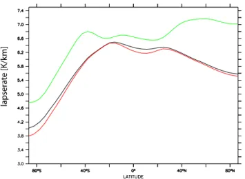
lapser

at

e [K/k

m]

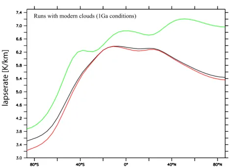
Fig. 6. Lapse rates (annual mean) calculated by CLIMBER lapse rate formula and FOAM using 1 Ga conditions (no clouds). Black curve represents the standard formulation in CLIMBER (Petoukhov et al., 2000), the red line is the calculation adapted for a faster ro-tation in CLIMBER (Kienert et al., 2012, 2013). The green line represents the FOAM lapse rate.

governs the sensitivity of climate to CO2 so that the

green-house effect (G) is expressed as

G(W m−2) = σTs4−OLR, (7)

where Ts is the surface temperature (K), σ the Stefan– Boltzmann constant. OLR corresponds to the energy lost by the Earth as infrared radiation at the top of the atmosphere.

The CLIMBER lapse rate is based on a theoretical ap-proach (Petoukhov et al., 2000) and was developed to fit em-pirical data such as

lapse rate = 00+01(Ts − 273.16 K) ∗ (1 − aq∗Q2)

−02∗ncld, (8)

where 00, 01 and 02 are lapse rate parameters (00

= 5.2 × 10−3 K m−1, 01 = 5.5 × 10−5K m−1, 02 =

10−3K m−1), Q is the surface-specific humidity (kg kg−1),

ncld the cumulus cloud amount and aq= 103 (kg kg)−2.

Kienert et al. (2012, 2013) updated this formula to ac-count explicitly for a faster Earth rotation rate such as

00 = 5.1 × 10−3K m−1, 01 = 6.1 × 10−5K m−1, 02 =

0.9−3K m−1 and aq = 1.171 × 103 (kg kg)−2. To

illus-trate CLIMBER lapse rate parameterisation better, we used FOAM outputs (i.e. Ts and Q). To suppress the cloud ef-fects, we extracted outputs from a run performed at 1 Ga with no clouds; therefore ncldis fixed to 0 (lapse rates

com-puted with clouds are available in Appendix Fig. A3). In CLIMBER the radiative transfer depends on Ht (troposphere height), so we calculated lapse rates for the entire tropo-sphere (from the Earth’s surface to an atmospheric pressure level of 254 mbar).

Figure 6 shows lapse rates for different case scenar-ios: (1) with the standard formula implemented in CLIMBER

(Petoukhov et al., 2000), (2) using the adapted formula in case of a faster rotation (Kienert et al., 2012, 2013) and (3) using FOAM. For the same values of Ts and Q, we show that the lapse rate is systematically underestimated with CLIMBER, hence inducing warmer temperature and a higher thermal radiation flux loss at the tropopause (the un-usual shape of the lapse rate is explained by the northern hemisphere which is almost entirely oceanic, see Fig. 2b). Therefore, for the same pCO2, CLIMBER results in a less

efficient greenhouse effect. This artefact in the CLIMBER lapse rate explains why this EMIC needs such a large pCO2

when a present-day Earth rotation is considered (Kienert at al., 2012). The required pCO2is even higher when a faster

Earth rotation is imposed. Although the authors discussed the uncertainties linked to CLIMBER radiative module (Kienert et al., 2013), they omitted lapse rate/OLR interplays. In ad-dition to possible effects of ocean and sea ice dynamics and an ice albedo above classical values, this omission could ex-plain why Kienert et al. (2012, 2013) proposed such a high

pCO2to solve the FYSP.

5.2 Pan-glaciation thresholds and ice-albedo feedback: AGCMs versus RCMs

It is noteworthy that atmospheric GCMs are able to main-tain a large fraction of open oceans (i.e. above the seawa-ter freezing point) with very moderate amounts of green-house gases, 0.9 mbar of CO2and CH4for LMDz (3.8 Ga),

3.7 mbar of CO2for EMAC (3.5 Ga) and 5 mbar of CO2for

CAM3 (2.7 Ga), a result that contrasts with RCM estimates (0.04 bar of CO2 at 3.5 Ga, Kasting, 1987). RCMs assume

that a drop of the mean temperature below 0◦_{C leads to a}

run-away glaciation, and therefore induces high pCO2in order

to maintain ice-free oceans during the Archaean. However, stable climates have been simulated using AGCMs while the global mean surface temperature falls well below 0◦C (Char-ney et al., 2013; Wolf and Toon, 2013; Kunze et al., 2014, this study). Wolf and Toon (2013) suggested that the differ-ence in the temperature leading to a runaway glaciation was the reason for the high estimates of pCO2by RCMs.

To better understand why RCMs are not able to calcu-late the threshold temperature allowing the onset of run-away glaciations, we implemented an albedo dependency on temperature in the RCM developed by MacKay and Khalil (1991). It should be noted that Wang and Stone (1980) incorporated this process, but for unknown reasons, all RCM experiments kept a surface albedo held constant. This lack had biased the climate response and the Earth was main-tained unfrozen for unrealistic reasons. To represent the ice-albedo feedback, we used the formula given by Pierrehum-bert et al. (2011) where the Earth albedo is assumed to be

– Ice-free for T > T0=20◦C, with an albedo (αo) =0.2 – Totally ice covered for T < Tfreeze, with an albedo

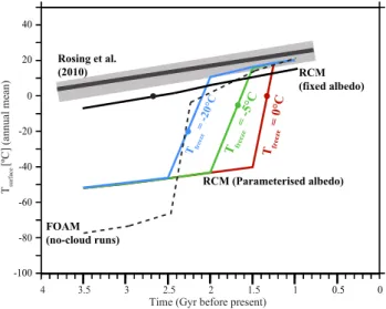
Time (Gyr before present) Tsurface [ºC] (annual mean) 4 3.5 3 2.5 2 1.5 1 0.5 0 Tfreeze = -20°C Tfreeze = -5°C Tfreeze = 0°C Rosing et al. (2010) RCM (fixed albedo) RCM (Parameterised albedo) FOAM (no-cloud runs) -100 -80 40 20 0 -20 -40 -60

Fig. 7. RCM simulations showing the evolution of the surface tem-perature versus time between 3.5 and 1 Ga, with and without the ice-albedo feedback, and assuming increasing irradiance in the

ab-sence of clouds and a greenhouse radiative forcing of 19 W m−2.

Blue, green and red curves were obtained using the ice-albedo

feed-back formula from Pierrehumbert et al. (2011) where Tfreezevalues

(−20◦C, −5◦C, 0◦C) represent the freezing temperature for the

Earth (snowball Earth threshold). The black curve is obtained using a surface albedo fixed at 0.264 (absence of ice-albedo feedback). Rosing et al. (2010) and FOAM runs are described in Fig. 3.

– Partially ice covered for Tfreeze< T < T0, the albedo is

interpolated according to the formula:

α(T ) = αo+(αfreeze−αo)[(T − T0)2/(Tfreeze−T0)2] (9)

where T is the Earth’s temperature and Tfreezeis the

thresh-old temperature for the onset on global glaciations. The dif-ference between Tfreezeand T0is a measure of the meridional

temperature gradient and therefore represents the efficiency of latitudinal heat transport. Because Wolf and Toon (2013) proposed that the freezing temperature is the main factor ex-plaining differences between RCMs and AGCMs, we tested several Tfreeze values (−20◦C, −5◦C, 0◦C). To avoid the

difficulty of figuring out how to represent cloud changes between FOAM and RCM we removed clouds, so that the albedo corresponds to the planetary albedo incorporating the effects of Rayleigh scattering, atmospheric solar absorption and the reflective properties of the surface.

The RCM and FOAM are forced with the same bound-ary conditions, that is a net radiative forcing of +19 W m−2

and no clouds. In the absence of the ice-albedo feedback (α = 0.264), the RCM simulates a linear increase in the mean temperature through time, the threshold value of 0◦C (sup-posed to represent the threshold temperature for runaway glaciations) being reached at about 2.6 Ga (Fig. 7). In con-trast, RCM experiments that include the ice-albedo feedback show a drastic shift in the evolution of the mean temperature

through time, similar to the one observed in FOAM experi-ments. More interestingly, when the ice-albedo feedback is parameterised such as the threshold temperature for the on-set of snowball Earth (Tfreeze)equals −20◦C, the timing of

the shift from snowball Earth to ice-free conditions is simi-lar in RCM and FOAM experiments. This simisimi-larity occurs because RCM mimics the latitudinal air surface temperature gradient of FOAM (1T = 40◦C from equator to 45◦of lat-itudes – sea ice latlat-itudes). This calculation illustrates an es-sential weakness of RCM: their inability to calculate Tfreeze

in the absence of latitudinal heat transport. In AGCMs, Tfreeze

varies with the prescribed boundary conditions (for example in FOAM, the maximum latitudinal extent of the ice cap be-fore the shift to runaway glaciation varies from 30◦ to 45◦ and 70◦ for experiments using modern clouds, cloud-free, and large-droplet clouds, respectively). This extent is con-trolled by the change in ocean heat flux, a process which can-not be captured by RCMs. Faster rotation and saltier oceans also slightly affect Tfreeze. Consequently, AGCMs, in contrast

to RCMs, more faithfully represent the ice-albedo feedback and hence the climatic transition towards snowball Earth.

5.3 Pan-glaciation thresholds and ice-albedo feedback: FOAM versus other AGCMs

The recent use of atmospheric GCMs for investigating the FYSP offered a great opportunity to compare FOAM with CAM3 (Wolf and Toon, 2013) LMDz (Charney et al., 2013) and EMAC (Kunze et al., 2014). All these studies suggested that Earth is less prone to full glaciations. Using a 2.7 Ga-old solar constant of 1093 W m−2_{and 1 mbar of CO}

2 and CH4

(other parameters being held at present-day values), CAM3 simulates a mean surface temperature close to 2◦_{C (Wolf and}

Toon, 2013). For the same conditions, FOAM yields a full glaciation. A small difference in ice albedo of 0.68(vis)/0.3 (nearIR) with CAM3 and 0.7(vis)/0.5(nearIR) with FOAM seems to explain the different behaviour. Although minor, this difference has important consequences on the impact of the ice-albedo feedback when Earth becomes ice-covered (ice line spreads down to 30–40◦; run 7 of Table 2). Using a 3 Ga-old solar constant (1082 W m−2)and 0.9 mbar of CO2,

LMDz does not simulate a full glaciation (Charney et al., 2013). This behaviour arises from both the prescribed bound-ary conditions and heat transport. Charney et al. (2013) made the hypothesis that Earth was an aquaplanet at 3 Ga. In such conditions, LMDz simulates larger amount of water vapour, which enhances heat transport to high latitudes and decreases the equator-pole temperature gradient, so that the ice-albedo feedback becomes less efficient and the runaway glaciation is delayed. This result is in good agreement with the result of Kunze et al. (2014) who also assumed a water-covered world for the early Archaean (3.5 Ga, solar constant 1046 W m−2). Using EMAC, they showed that it was possible to get a stable ice-free ocean at low latitudes (surface temperature equals to −9◦C) with moderate CO2concentrations (3670 ppmv).

708 G. Le Hir et al.: The faint young Sun problem

For comparison, LMDz prevents the early Earth (3.8 Ga, 1025 W m−2_{)from completely freezing with a greenhouse}

forcing corresponding to 0.9 mbar of a CO2 combined to

0.9 mbar of CH4(Charney et al., 2013).

LMDz simulations also investigated the effect of CCN. Performing simulations with larger droplets (droplet radius set to 17 instead of 20 µm in our study), Charney et al. (2013) suggested a strong impact on the terrestrial radiative bud-get, in agreement with this study. More interestingly, both AGCMs simulate an increase in the cloud water path in low-altitude clouds located at high latitudes. Since the use of these two different cloud schemes shows similar behaviour, we suspect that the warming driven by high-latitude clouds inhibiting sea ice formation is not model dependent (see Sect. 3.4).

Other processes such as pressure broadening of CO2and

H2O by high atmospheric pressure (Goldblatt et al., 2009)

or high concentrations of H2 (Wordsworth and

Pierrehum-bert, 2013), which are not treated here, could also warm up the early Earth and affect the FYSP solutions. In addition, several processes are missing in this study, which are poten-tial sources of uncertainties. The use of a slab ocean, with heat transport parameterised through diffusion, precludes the faithful representation of the meridional ocean heat port. Indeed, during the Archaean the oceanic heat trans-port should supposedly be enhanced due to the smaller land fraction (Endal and Schatten, 1982). We also acknowledge that saltier oceans possibly lead to a weaker overturning (Williams et al., 2010). These conflicting assessments con-cerning ocean circulation, and their respective influence on the FYSP, could be explored using a fully coupled dynamic ocean model, an investigation which has not been conducted here. The last limitation relative to the use of a slab ocean is the absence of sea ice dynamics, which tends to slow the sea ice flow (Voigt and Abbot, 2012). This lack may change the radiative deficit triggering the onset of pan-glaciation and underestimate the greenhouse gas concentrations required to keep the early Earth unfrozen.

Obviously atmospheric GCMs still have limitations (Hack, 1998; Abbot et al., 2012; Stevens and Bony, 2013) and re-sults can slightly differ according to their respective param-eterisations or boundary conditions. However, as fully dy-namic models, AGCMs represent a powerful tool for improv-ing our understandimprov-ing of deep past Earth climates, capturimprov-ing cloud mechanisms involved in global warming, as well as time-dependent factors (e.g. palaeogeography, rotation rate). However, constraints on paleo-pCO2 gained from climate

modelling studies cannot be directly compared to geologi-cal data because all these studies omit to consider the car-bon cycle-climate equilibrium. To estimate more accurately

pCO2and the Earth’s surface temperature evolution, we

as-sociated the atmospheric GCM simulations discussed in this paper with a geochemical model to investigate the carbon cy-cle climate during the Archaean (see companion paper).

6 Conclusions

FOAM, like other AGCMs, suggests a faint young Sun prob-lem less probprob-lematic than initially assumed and solves the FYSP with a composition of greenhouse gases one order a magnitude lower than RCM or EMIC. Accounting for a 23 % weaker Sun at 3.5 Ga, we show that a moderate radia-tive forcing of 41 W m−2 is sufficient to maintain the mean global surface temperature close to its present-day value. As-suming a high pCH4in the Archaean atmosphere (Pavlov et

al., 2000; Catling et al., 2007), we show that such a moder-ate radiative forcing can be provided by the combination of 1 (0.3) mbar of methane and 11.5 (16) mbar of carbon dioxide. The presence of large-droplet clouds can theoretically pro-vide significant warming so that lower CO2and CH4partial

pressures are required for the maintenance of an ice-free sur-face. We demonstrated, however, that such changes in cloud properties cannot alone provide sufficient warming to solve the FYSP with low (0.9 mbar) pCO2as defended by Rosing

et al. (2010).

This study highlights the central role of AGCMs over RCMs in investigating glacial thresholds. RCMs overesti-mate the early Archaean pCO2 (i.e. 0.2–0.3 bar) required

to keep equatorial waterbelts ice free due to their inabil-ity to calculate the correct threshold mean temperature for the onset of full glaciation (i.e. Tfreeze). Applying Archaean

boundary conditions, our AGCM simulations show a wide range of possible values for Tfreeze, from −20 to 13◦C,

ac-cording to the latitudinal temperature gradient. In contrast, RCMs use a fixed Tfreeze value (0◦C, the freezing point

of seawater) and therefore inaccurately estimate the pole-ward heat transport. The weak sensitivity of CLIMBER to CO2could be explained by its lapse rate calculation, which

overestimates the energy leaving the Earth as infrared ra-diation. Our AGCM supports the main conclusions arising from previous AGCMs, but predicts an early Earth more in-clined to full glaciation. Higher ice albedo is a likely cause for the stronger ice-albedo feedback in FOAM compared to CAM3. LMDz and EMAC simulate warmer climate due to a weaker ice-albedo feedback inherited from the absence of continents, a boundary condition that enhances poleward moist heat fluxes. However, all these studies cannot simu-late ocean and sea ice dynamics, a limitation which may un-derestimate the greenhouse gas concentrations required to keep the early Earth unfrozen. Following this step forward in the understanding of physical processes able to solve the FYSP, we now consider carbon cycle–climate interplays to provide a complete picture of the faint young Sun problem (companion paper).

Acknowledgements. We thank the two anonymous referees for

their very insightful reviews which considerably improved the quality of the manuscript, and the editorial board for the quality of the review procedure. This work was granted access to the HPC resources of CCRT under allocation 2014-017013 made

by GENCI (Grand Equipement National de Calcul Intensif). This work was supported by ANR eLIFE2 and LabexUnivEarth (ANR-10-LABX-0023 and ANR-11-IDEX-0005-02). This is IPGP contribution 3494.

Edited by: M. Claussen

The publication of this article is financed by CNRS-INSU.

References

Abbot, D. S., Voigt, A., Branson, M., Pierrehumbert, R. T., Pollard, D., Le Hir, G., and Koll, D. D. B.: Clouds and snowball Earth deglaciation, Geophys. Res. Lett., 39, L20711, doi:10.1029/2012GL052861, 2012.

Andreae, M. O. and Rosenfeld, D.: Aerosol–cloud–

precipitation interactions. Part 1. The nature and sources

of cloud-active aerosols, Earth-Sci. Rev., 89, 13–41,

doi:10.1016/j.earscirev.2008.03.001, 2008.

Boucher, O., Le Treut, H., and Baker, M. B.: Precipitation and ra-diation modeling in a general circulation model: Introduction of cloud microphysical processes, J. Geophys. Res., 100, 16395– 16414, doi:10.1029/95JD01382, 1995.

Bréon, F. M., Tanré, D., and Generoso, S.: Aerosol Effect on Cloud Droplet Size Monitored from Satellite, Science, 295, 834–838, doi:10.1126/science.1066434, 2002.

Catling, D. C., Claire, M. W., and Zahnle, K. J.: Anaerobic methan-otrophy and the rise of atmospheric oxygen, Phil. Trans. R. Soc., 365, 1867–1888, doi:10.1098/rsta.2007.2047, 2007.

Charlson, R. J., Lovelock, J. E., Andreae, M. O., and Warren, S. G.: Oceanic Phytoplankton, atmospheric sulfur, cloud albedo and climate, Nature, 326, 655–661, 1987.

Charney, B., Forget, F., Wordworth, R., Leconte, J., Millour, E., Co-dron, F., and Spiga, A.: Exploring the faint young Sun problem and the possible climates of the Archean Earth with a 3-D GCM, J. Geophys. Res., 118, 10414–10431, doi:10.1002/jgrd.50808, 2013.

Dauphas, N. and Kasting, J. F.: Low pCO2in the pore water, not in

the Archean air, Nature, 474, E2–E3, doi:10.1038/nature09960, 2011.

Driese, S. G., Jirsa, M. A., Ren, M., Brantley, S. L., Shel-don, N. D., Parker, D., and Schmitz, M.: Neoarchean pa-leoweathering of tonalite and metabasalt: implicationsq for reconstructions of 2.69 Ga early terrestrial ecosystems and paleoatmospheric chemistry, Precambrian Res., 187, 1–17, doi:10.1016/j.precamres.2011.04.003, 2011.

Farquhar, J., Airieau, S., and Thiemens, M. H.: Observation of wavelength-sensitive mass-independent sulfur isotope effects

during SO2 photolysis: Implications for the early atmosphere,

J. Geophy. Res.-Planets, 106, 32829–32839, 2001.

Feulner, G.: The faint young sun problem, Rev. Geophys., 50, RG2006, doi:10.1029/2011RG000375, 2012.

Foriel, J., Philippot, P., Rey, P., Somogyi, A., Banks, D., and Menez, B.: Biological control of Cl/Br and low sulfate concentration in a 3.5-Gyr-old seawater from North Pole, Western Australia, Earth Planet. Sci. Lett., 228, 451–463, 2004.

Godderis, Y. and Veizer, J.: Tectonic control of chemical and iso-topic composition of ancient oceans: the impact of continental growth, Am. J. Sci., 300, 434–461, 2000.

Goldblatt, C. and Zahnle, K. J.: Faint Young Sun Paradox remains, Nature, 474, E1, doi:10.1038/nature09961, 2011a.

Goldblatt, C. and Zahnle, K. J.: Clouds and the Faint Young Sun Paradox, Clim. Past, 7, 203–220, doi:10.5194/cp-7-203-2011, 2011b.

Goldblatt, C., Claire, M. W., Lenton, T. M., Matthews, A. J., Watson. A. J., and Zahnle, K. J.: Nitrogen-enhanced green-house warming on early Earth, Nat. Geosci., 2, 891–896, doi:10.1038/NGEO692, 2009.

Gough, D. O.: Solar interior structure and luminosity variations, Sol. Phys., 74, 21–34, 1981.

Hack, J. J.: Sensitivity of the simulated climate to a diagnostic for-mulation for cloud liquid water, J. Climate, 11, 1497–1515, 1998. Halevy, I., Pierrehumbert, R. T., and Schrag, D. P.: Radiative

transfer in CO2-rich paleoatmospheres, J. Geophys. Res., 114,

D18112, doi:10.1029/2009JD011915, 2009.

Hansen, J., Sato, M., and Ruedy, R.: Radiative Forcing and climate response, J. Geophys. Res., 102, 6831–6864, 1997.

Haqq-Misra, J. D., Domagal-Goldman, S. D., Kasting, P. J., and Kasting, J. F.: A revised, hazy methane greenhouse for the archean Earth, Astrobiology, 8, 1127–1137, 2008.

Jacob, R.: Low frequency variability in a simulated atmosphere ocean system, PhD Thesis, University of Wisconsin-Madison, 1997–310, 1997.

Jenkins, G. S.: The effects of reduced land fraction and solar forcing on the general circulation results from the NCAR CCM, Glob. Planet. Change, 7, 321–333, 1993a.

Jenkins, G. S.: A General Circulation Model Study of the Effects

of Faster Rotation Rate, Enhanced CO2Concentration, and

Re-duced Solar Forcing’ Implications for the Faint Young Sun Para-dox, J. Geophys. Res., 98, 20803–20811, 1993b.

Jenkins, G. S., Marshall, H. G., and Kuhn, W. R.: Precambrian climate – the effects of land area and Earth’s rotation rate, J. Geophys. Res.-Atmos., 98, 8785–8791, doi:10.1029/93JD00033, 1993.

Kasting, J. F.: The evolution of the prebiotic atmosphere, Origins Life Evol. B., 14, 75–82, 1984.

Kasting, J. F.: Theoretical constraints on oxygen and carbon-dioxide concentrations in the Pre-cambrian atmosphere, Precambrian Res., 34, 205–229, 1987.

Kasting, J. F.: Early Earth faint young sun redux, Nature, 464, 687– 689, 2010.

Kiehl, J. T. and Dickinson, R. E.: A study of the radiative effects

of enhanced atmospheric CO2and CH4on early Earth surface

temperatures, J. Geophys. Res.-Atmos., 92, 2991–2998, 1987. Kienert, H., Feulner, G., and Petoukhov, V.: Faint young sun

prob-lem more severe due to ice-albedo feedback and higher rota-tion rate of the early Earth, Geophys. Res. Lett., 39, L23710, doi:10.1029/2012GL054381, 2012.

710 G. Le Hir et al.: The faint young Sun problem

Kienert, H., Feulner, G., and Petoukhov, V.: Albedo and heat trans-port in 3-D model simulations of the early Archean climate, Clim. Past, 9, 1841–1862, doi:10.5194/cp-9-1841-2013, 2013. Knauth, L. P.: Temperature and salinity history of the Precambrian

ocean: implications for the course of microbial evolution, Palaeo-geogr. Palaeocl., 219, 53–69, 2005.

Kump, L. R. and Pollard, D.: Amplification of cretaceous warmth by biological cloud feedbacks, Science, 320, 195–195, 2008. Kunze, M., Godolt, M., Langematz, U., Grenfell, J. L.,

Hamann-Reinus, A., and Rauer, H.: Investigating the early Earth faint young Sun problem with a general circulation model, Planet. Space Sci., doi:10.1016/j.pss.2013.09.011, in press, 2014. Le Hir, G., Donnadieu, Y., Krinner, G., and Ramstein, G.: Toward

the snowball earth deglaciation, Clim. Dynam., 35, 285–297, 2010.

Lowe, D. R. and Tice, M. M.: Tectonic controls on atmospheric, climatic, and biological evolution 3.5–2.5 Ga, Precambrian Res., 158, 177–197, 2007.

MacKay, R. M. and Khalil, M. A. K.: Theory and Development of a One Dimensional Time Dependant Radiative Convective Climate Model, Chemosphere, 22, 383–417, 1991.

Millero, F. J. and Poisson, A.: International one-atmosphere equa-tion of state of seawater, Deep-Sea Res. Pt. I, 28, 625–629, 1981. Pavlov, A. A., Kasting, J. F., Brown, L. L., Rages, K. A., and

Freed-man, R.: Greenhouse warming by CH4in the atmosphere of early

Earth, J. Geophys. Res.-Planets, 105, 11981–11990, 2000. Penner, J. E., Quaas, J., Storelvmo, T., Takemura, T., Boucher, O.,

Guo, H., Kirkevåg, A., Kristjánsson, J. E., and Seland, Ø.: Model intercomparison of indirect aerosol effects, Atmos. Chem. Phys., 6, 3391–3405, doi:10.5194/acp-6-3391-2006, 2006.

Petoukhov, V., Ganopolski, A., Brovkin, V., Claussen, M., Eliseev, A., Kubatzki, C., and Rahmstorf, S.: CLIMBER-2: a climate sys-tem model of intermediate complexity. Part I: model description and performance for present climate, Clim. Dynam. 16, 1–17, doi:10.1007/PL00007919, 2000.

Pesonen, L. J., Elming, S. A, Mertanen, S., Pisarevsky, S., D’Agrella-Filho, M. S., Meert, J. G., Schmidt, P. W., Abraham-sen, N., and Bylund, G.: Palaeomagnetic configuration of con-tinents during the Proterozoic, Tectonophysics, 375, 289–324, 2003.

Pierrehumbert, R. T.: High levels of atmospheric carbon dioxide necessary for the termination of global glaciation, Nature, 429, 646–649, 2004.

Pierrehumbert, R. T.: Principles of Planetary Climate, Cambridge University Press, 652 pp., 2010.

Pierrehumbert, R. T., Abbot, D. S., Voigt., A., and Koll, D.: Climate of the Neoproterozoic Annual, Rev. Earth Planet. Sci., 39, 417– 460, doi:10.1146/annurev-earth-040809-152447, 2011. Reinhard, C. T. and Planavsky, N. J.: Mineralogical

con-straints on Precambrian pCO2, Nature, 474, E1–E2,

doi:10.1038/nature09959, 2011.

Rosing, M. T., Bird, D. K., Sleep, N. H., and Bjerrum, C. J.: No climate paradox under the faint early Sun, Nature, 464, 744–747, doi:10.1038/nature08955, 2010.

Rye, R., Kuo, P. H., and Holland, H. D.: Atmospheric carbon-dioxide concentrations before 2.2-billion years ago, Nature, 378, 603–605, 1995.

Sagan, C. and Mullen, G.: Earth and Mars – evolution of at-mospheres and surface tempera-tures, Science, 177, 52–56, doi:10.1126/science.177.4043.52, 1972.

Schatten, K. H. and Endal, A. S.: The faint young Sun climate para-dox – volcanic influence, Geophys. Res. Lett., 9, 1309–1311, doi:10.1029/GL009i012p01309, 1982.

Sheldon, N. D.: Precambrian paleosols and atmospheric CO2levels,

Precambrian Res., 147, 148–155, 2006.

Slingo, A.: A GCM parameterization for the shortwave radiative properties of water clouds, J. Atmos. Sci., 46, 1419–1427, 1989. Stevens, B. and Bony, S.: What Are Climate Models Missing?,

Sci-ence, 340, 1053–1054, doi:10.1126/science.1237554, 2013. Voigt, A. and Abbot, D. S.: Sea-ice dynamics strongly promote

Snowball Earth initiation and destabilize tropical sea-ice mar-gins, Clim. Past, 8, 2079–2092, doi:10.5194/cp-8-2079-2012, 2012.

von Paris, P., Rauer, H., Grenfell, J. L., Patzer, B., Hedelt, P., Stracke, B., Trautmann, T., and Schreier, F.: Warming the early

earth-CO2 reconsidered, Planet. Space Sci., 56, 1244–1259

doi:10.1016/j.pss.2008.04.008, 2008.

Walker, J. C. G.: Climatic factors on the Archean Earth, Palaeogr. Palaeocl., 40, 1–11, doi:10.1016/0031-0182(82)90082-7, 1982. Walker, J. C. G. and Zahnle, K. J. Lunar nodal tide and distance to

the Moon during the Pre-cambrian, Nature, 320, 600–602, 1986. Walker, J. C. G., Hays, P. B., and Kasting, J. F.: A Nega-tive Feedback Mechanism For The Long-Term Stabilization of Earth’s Surface-Temperature, J. Geophys. Res.-Ocean. Atmos., 86, 9776–9782, 1981.

Wang, W. and Stone, P. H.: Effect of Ice-Albedo Feedback on Global Sensitivity in a One-Dimensional Radiative-Convective Climate Model, J. Atmophs. Sci., 37, 545–552, 1980.

Warren, S. G., Brandt, R. E., Grenfell, T. C., and McKay, C. P.: Snowball Earth: Ice thickness on the tropical ocean, J. Geophys. Res.-Ocean., 107, 31-1–31-18, doi:10.1029/2001JC001123, 2002.

Williams, P. D., Guilyardi, E., Madec, G., Gualdi, S.,

and Scoccimarro, E.: The role of mean ocean

salin-ity in climate, Dynam. Atmos. Oceans, 49, 108–123,

doi:10.1016/j.dynatmoce.2009.02.001, 2010.

Wolf, E. T. and Toon, O. B.: Hospitable Archean Climates Sim-ulated by a General Circulation Model, Astrobiology, 13, 656– 673, doi:10.1089/ast.2012.0936, 2013.

Wordsworth, R. and Pierrehumbert, R.: Hydrogen-nitrogen green-house warming in Earth’s early atmosphere, Science, 339, 64–67, doi:10.1126/science.1225759, 2013.

Appendix A

modern Earth rotation rate 3.5Ga Earth rotation rate (16h of daylength)

100

Atmospheric Pressure [hPa]

300 500 700 900 Air Temperature [°C] 0 20 -20 -40 -60 -80 -100 -120 -140 Surface temperature [°C] Latitude a) _b)

modern lapse rate modern lapse rate without ozone layer

Fig. A1. (a) Temperature gradient as a function of Earth rotation rates. (b) Atmospheric lapse rate as a function of ozone layer pres-ence/removal. Simulations performed under present-day boundary conditions.