HAL Id: hal-02109189
https://hal.archives-ouvertes.fr/hal-02109189
Submitted on 24 Apr 2019
HAL is a multi-disciplinary open access
archive for the deposit and dissemination of
sci-entific research documents, whether they are
pub-lished or not. The documents may come from
teaching and research institutions in France or
abroad, or from public or private research centers.
L’archive ouverte pluridisciplinaire HAL, est
destinée au dépôt et à la diffusion de documents
scientifiques de niveau recherche, publiés ou non,
émanant des établissements d’enseignement et de
recherche français ou étrangers, des laboratoires
publics ou privés.
The HARPS search for southern extra-solar planets.
XLII. Eight HARPS multi-planet systems hosting 20
super-Earth and Neptune-mass companions
S. Udry, X. Dumusque, C. Lovis, D. Segransan, R Diaz, W. Benz, F. Bouchy,
A Coffinet, G Curto, M. Mayor, et al.
To cite this version:
S. Udry, X. Dumusque, C. Lovis, D. Segransan, R Diaz, et al.. The HARPS search for southern
extra-solar planets. XLII. Eight HARPS multi-planet systems hosting 20 super-Earth and Neptune-mass
companions. Astronomy and Astrophysics - A&A, EDP Sciences, 2019. �hal-02109189�
January 29, 2019
The HARPS search for southern extra-solar planets.
XLII. Eight HARPS multi-planet systems hosting 20 super-Earth and
Neptune-mass companions
? ?? ???S. Udry
1, X. Dumusque
1, C. Lovis
1, D. Ségransan
1, R.F. Diaz
1, W. Benz
2, F. Bouchy
1, 3, A. Coffinet
1, G. Lo Curto
4,
M. Mayor
1, C. Mordasini
2, F. Motalebi
1, F. Pepe
1, D. Queloz
1, N.C. Santos
5, 6, A. Wyttenbach
1, R. Alonso
7, A. Collier
Cameron
8, M. Deleuil
3, P. Figueira
5, M. Gillon
9, C. Moutou
3, 10, D. Pollacco
11, and E. Pompei
41 Observatoire astronomique de l’Université de Genève, 51 ch. des Maillettes, CH-1290 Versoix, Switzerland 2 Physikalisches Institut, Universitat Bern, Silderstrasse 5, CH-3012 Bern, Switzerland
3 Aix Marseille Université, CNRS, LAM (Laboratoire d’Astrophysique de Marseille) UMR 7326, 13388, Marseille, France 4 European Southern Observatory, Karl-Schwarzschild-Str. 2, D-85748 Garching bei München, Germany
5 Instituto de Astrofísica e Ciências do Espaço, Universidade do Porto, CAUP, Rua das Estrelas, 4150-762 Porto, Portugal 6 Departamento de Física e Astronomia, Faculdade de Cièncias, Universidade do Porto, Rua do Campo Alegre, 4169-007 Porto,
Portugal
7 Instituto de Astrofisica de Canarias, 38025, La Laguna, Tenerife, Spain
8 School of Physics and Astronomy, University of St Andrews, North Haugh, St Andrews, Fife KY16 9SS
9 Institut d’Astrophysique et de Géophysique, Université de Liège, Allée du 6 Août 17, Bat. B5C, 4000, Liège, Belgium 10 Canada France Hawaii Telescope Corporation, Kamuela, 96743, USA
11 Department of Physics, University of Warwick, Coventry, CV4 7AL, UK Received XXX; accepted XXX
ABSTRACT
Context.We present radial-velocity measurements of eight stars observed with the HARPS Echelle spectrograph mounted on the 3.6-m telescope in La Silla (ESO, Chile). Data span more than ten years and highlight the long-term stability of the instrument. Aims.We search for potential planets orbiting HD 20003, HD 20781, HD 21693, HD 31527, HD 45184, HD 51608, HD 134060 and HD 136352 to increase the number of known planetary systems and thus better constrain exoplanet statistics.
Methods.After a preliminary phase looking for signals using generalized Lomb-Scargle periodograms, we perform a careful analysis of all signals to separate bona-fide planets from signals induced by stellar activity and instrumental systematics. We finally secure the detection of all planets using the efficient MCMC available on the Data and Analysis Center for Exoplanets (DACE web-platform), using model comparison whenever necessary.
Results.In total, we report the detection of twenty new super-Earth to Neptune-mass planets, with minimum masses ranging from 2 to 30 MEarthand periods ranging from 3 to 1300 days, in multiple systems with two to four planets. Adding CORALIE and HARPS measurements of HD20782 to the already published data, we also improve the characterization of the extremely eccentric Jupiter orbiting this visual companion of HD 20781.
Key words. Planetary systems – Techniques: RVs – Techniques: spectroscopy – Methods: data analysis – Stars: individual: HD 20003, HD 20781, HD 20782, HD 21693, HD 31527, HD 45184, HD 51608, HD 134060, HD 136352
1. Introduction
The radial velocity (RV) planet search programs with theHARPS
spectrograph on the ESO 3.6-m telescope (Pepe et al. 2000; Mayor et al. 2003) have contributed in a tremendous way to our
Send offprint requests to: Stéphane Udry, e-mail: [email protected]
?
Based on observations made with the HARPS instrument on the ESO 3.6 m telescope at La Silla Observatory under the GTO program 072.C-0488 and Large program 193.C-0972/193.C-1005/.
?? The analysis of the radial-velocity measurements were performed using the Data and Analysis Center for Exoplanets (DACE) developed in the frame of the Swiss NCCR PlanetS and available for the commu-nity at the following address: https://dace.unige.ch/
??? The HARPS RV measurements discussed in this paper are available in electronic form at the CDS via anonymous ftp to cdsarc.u-strasbg.fr (130.79.128.5) or via http://cdsweb.u-strasbg.fr/cgi-bin/qcat?J/A+A/.
knowledge of the population of small-mass planets around solar-type stars. The HARPS planet-search program on Guaranteed Time Observations (GTO, PI: M. Mayor) was on-going for 6 years between autumn 2003 and spring 2009. The high-precision part of thisHARPSGTO survey aimed at the detection of very low-mass planets in a sample of quiet solar-type stars already screened for giant planets at a lower precision with theCORALIE
Echelle spectrograph mounted on the 1.2-m Swiss telescope on the same site (Udry et al. 2000). The GTO was then continued within the ESO Large Programs 183.C-0972, 183.C-1005 and 192.C-0852 (PI: S. Udry), from 2009 to 2016.
Within these programs,HARPShas allowed for the detection (or has contributed to the detection) of more than 100 extra-solar planet candidates (see detections in Díaz et al. 2016a; Moutou et al. 2015; Lo Curto et al. 2013; Dumusque et al. 2011a; Mayor et al. 2011; Pepe et al. 2011; Moutou et al. 2011; Lovis et al.
2011b). In particular, HARPS has unveiled the existence of a large population of low-mass planets including super-Earths and hot Neptunes previous to the launch of the Kepler satellite which provided us with an overwhelming sample of thousands of small-size transiting candidates (Coughlin et al. 2016; Mullally et al. 2015; Borucki et al. 2011; Batalha et al. 2011). A preliminary analysis of theHARPSdata showed at that time that at least 30 % of solar-type stars were hosting low-mass planets on short-period orbits with less than 50 days (Lovis et al. 2009). A comprehen-sive analysis of our high-precision sample combined with 18 years of data fromCORALIEallowed us later to precise this oc-currence rate: about 50% of the stars surveyed have planets with masses below 50 M⊕on short to moderate period orbits (Mayor
et al. 2011). Furthermore, a large fraction of those planets are in multi-planetary systems. This preliminary statistics of hot super-Earth and Neptune frequency is now beautifully confirmed by the impressive results of the Kepler mission.
With the RV technique, the variation of the velocity of the central star due to the perturbing effect of small-mass planets becomes very small, of the order or even smaller than the un-certainties of individual measurements. The problems to solve and characterize the individual systems are then multi-fold, re-quiring to disentangle the planetary from the stellar, instrumen-tal, and statistical noise effects. Efficient statistical techniques, mainly based on a Bayesian approach, have been developed to optimise the process and thus the outcome of ongoing RV sur-veys (see e.g., Dumusque et al. 2016; Díaz et al. 2016b, and references therein). A large number of observations is however paramount for a complete probe of the planetary content of the system, and to take full advantage of the developed technique of analysis. In this context, focusing on the most observed, clos-est and brightclos-est stars, an on-goingHARPSLP (198.C-0836) is continuing the original observing efforts and providing us with an unprecedented sample of well observed stars. In this paper we describe 8 planetary systems hosting 20 planets. The detection of these planets has been announced in Mayor et al. (2011)1 study-ing statistical properties of the systems discovered withHARPS. Most of them are super-Earths and Neptunian planets on rela-tively short periods, and member of a multi-planet system. We present here the orbital solutions for one 4-planet system around
HD20781, three 3-planet systems aroundHD20003,HD31527 and HD136352, and four 2-planet systems around HD21693,
HD45184,HD51608, andHD134060. In addition, we give up-dated parameters for the very eccentric planet orbitingHD20782 (Jones et al. 2006), derived by combiningHARPS,CORALIEand the published UCLESdata. The paper is organised as follows. In Sec. 2 we discuss the primary star properties. Radial-velocity measurements and orbital solutions of each system are presented in Sects. 3 and 5, while Sec. 4 describes the framework used for analysing the data. We provide concluding remarks in Sec. 6.
2. Stellar characteristics
This section provides basic information about the stars hosting the planets presented in this paper. Effective temperature, grav-ity and metallicgrav-ity are derived from the spectroscopic analy-sis ofHARPS spectra and provided in Sousa et al. (2008). We used the improved Hipparcos astrometric parallaxes re-derived by van Leeuwen (2007) to determine the absolute V-band
mag-1 This paper presents the characterization of half of the planets an-nounced in Mayor et al. (2011). The latter paper was then waiting for the detailed analysis to be published before being resubmitted in parallel to the present paper.
nitude using the apparent visual magnitude from Hipparcos (ESA 1997). Metallicities, together with the effective temper-atures and MV are then used to estimate basic stellar
parame-ters (ages, masses) using theoretical isochrones from the grid of Geneva stellar evolution models, including a Bayesian estima-tion method (Mowlavi et al. 2012).
Individual spectra were also used to derive measurements of the chromospheric activity S-index, log(R0
HK) and Hα, following
a similar approach as used by Santos et al. (2000) and Gomes da Silva et al. (2011). Using Mamajek & Hillenbrand (2008), we es-timate rotational periods for our stars from the empirical correla-tion of stellar rotacorrela-tion and chromospheric activity index (Noyes et al. 1984). We also derived the v sin (i) from a calibration of the Full Width at Half Maximum (FWHM) of theHARPS Cross-Correlation Function (CCF) following a standard approach (e.g. Santos et al. 2002). All those extra indicators are used to dis-entangle small-amplitude planetary signals from stellar "noise" (see e.g. the cases of CoRoT-7 and α Centauri B; Queloz et al. 2009; Dumusque et al. 2012). The derived stellar parameters are summarized in Table 1.
3. HARPS RV measurements
Radial velocities presented here have been obtained with the
HARPShigh-resolution spectrograph installed on the 3.6m ESO telescope at La Silla Observatory (Mayor et al. 2003). The long-term m s−1RV precision is ensured by nightly ThAr calibrations (Lovis et al. 2008). On the short timescale of a night, the high precision is obtained using simultaneous ThAr (from 2003 to 2013) or Fabry-Perot étalon (since 2013) reference calibrations. The data reduction was performed with the latest version of the HARPS pipeline. In addition to the barycentric radial velocities with internal error bars, the reduction provides the Bisector In-verse Slope (BIS) of theHARPSCCF (Pepe et al. 2002; Baranne et al. 1996), as defined by Queloz et al. (2000), the FWHM and the Contrast of the CCF, as well as the Ca II activity indexes S and log(R0
HK).
By construction of the HARPShigh-precision sample from low-activity stars in theCORALIEvolume-limited planet-search sample, the eight stars discussed here present low activity lev-els. The average values of the log(R0
HK) activity index, estimated
from the chromospheric re-emission in the Ca II H and K lines at λ= 3933.66 Å and 3968.47 Å, are low, ranging from −5.01 to −4.87. Activity-induced RV jitter on stellar rotation time scales, due to spots and faculae on the stellar surface, is thus expected to remain at a low level. The potential influence of stellar activity on RVs is nevertheless scrutinised closely when long-term vari-ation of activity indexes are observed (magnetic cycle) or when the planetary and stellar rotation periods (or harmonics) are of similar values.
Low-mass planets are very often found in multi-planet sys-tems (e.g. Lovis et al. 2006, 2011b; Udry & Santos 2007; Mayor et al. 2009; Vogt et al. 2010; Díaz et al. 2016b; Motalebi et al. 2015; Latham et al. 2011; Lissauer et al. 2011, 2014; Fabrycky et al. 2014, for examples of RV results and Kepler findings). The several components in the system give rise to often complex, low-amplitude RV signals, not easy to solve for. The optimal ob-serving strategy for a given star is a priori unknown, the relevant planetary periods possibly extending over three orders of mag-nitude. An adequate and efficient observing strategy has been developed coping with the need to accumulate a large number of measurements and to probe different timescales of variation. We typically follow our targets every night during a few initial
Table 1. Observed and inferred stellar parameters for the stars hosting planetary systems described in this paper. Parameters HD 20003 HD 20781a HD 21693 HD 31527 HD 45184 HD 51608 HD 134060 HD 136352 Sp. Type(1) G8V K0V G8V G2V G1.5V G7V G3IV G4V V(1) 8.39 8.48 7.95 7.49 6.37 8.17 6.29 5.65 B − V(1) 0.77 0.82 0.76 0.61 0.62 0.77 0.62 0.63 π [mas](1) 22.83±0.65 28.27±1.08 30.88±0.49 25.93±0.60 45.70±0.40 28.71±0.51 41.32±0.45 67.51±0.39 MV(1) 5.22 5.70 5.40 4.87 4.65 5.51 4.38 4.83 Teff[K](2) 5494±27 5256±29 5430±26 5898 ±13 5869±14 5358±22 5966±14 5664±14 [Fe/H](2) 0.04 ± 0.02 −0.11 ± 0.02 0.0 ± 0.02 −0.17 ± 0.01 0.04 ± 0.01 −0.07 ± 0.01 0.14 ± 0.01 −0.34 ± 0.01 log (g)(2) 4.41±0.05 4.37±0.05 4.37 ±0.04 4.45±0.02 4.47±0.02 4.36±0.05 4.43 ±0.03 4.39±0.02 M?[M ](2) 0.875 0.70 0.80 0.96 1.03 0.80 1.095 0.81 L?[L ](2) 0.72±0.03 0.49±0.04 0.62±0.02 1.20±0.03 1.13±0.01 0.57±0.02 1.44±0.02 0.99±0.01 log(R0 HK) (3) −4.97±0.05 −5.03±0.01 −4.91±0.05 −4.96±0.01 −4.91±0.01 −4.98±0.02 −5.00±0.01 −4.95±0.01 v sin (i) [km s−1](3) 1.9 1.1 1.6 1.9 2.1 1.3 2.6 < 1 Prot[days](4) 38.9±4.0 46.8±4.4 35.2±4.0 20.3±2.9 21.5±3.0 40.0±4.0 23.0±2.9 23.8±3.1
Notes. (1) Astrometric and visual photometric data from the Hipparcos Catalogs (ESA 1997; van Leeuwen 2007). (2) From Sousa et al. (2008) spectroscopic analysis. (3) Parameter derived using HARPS spectra or CCF. (4) From the calibration of Mamajek & Hillenbrand (2008). aHD 20782, the stellar visual companion of HD 20781, hosts a planet as well. The corresponding stellar parameters are given in Jones et al. (2006).
Table 2. General statistics of the HARPS observations of the planet-host stars presented in this paper, with the number of individual spectra observed, <S/N> the average signal-to-noise ratio at 550 nm of those spectra, the number of measurements obtained after binning the data over 1 hour,∆T the time span of the observations, σRVthe rms value of the RV set and < εRV> the mean RV photon-noise + calibration error.
Nspectr < SNR > Nmeas ∆T σRV < εRV>
550 nm 1-hour bin [days] [m/s] [m/s]
HD 20003 184 110 184 4063 5.35 0.74 HD 20781 225 112 216 4093 3.41 0.76 HD 20782a 71 181 68 4111 36.86 0.56 HD 21693 210 141 210 4106 4.72 0.60 HD 31527 256 180 245 4135 3.19 0.64 HD 45184 308 221 178 4160 4.72 0.41 HD 51608 218 133 216 4158 4.07 0.62 HD 134060 335 199 155 4083 3.68 0.40 HD 136352 649 231 240 3993 2.74 0.33
Notes.aStar already known as a planet host for which we give here an updated orbit including HARPS observations.
observing runs, and after gathering a couple of dozens of obser-vations we compare the observed dispersion with the expected jitter for the considered stellar spectral type. For significant vari-ations we then continue monitoring at the same cadence when high-frequency variations are seen, or we adapt the frequency to possible variations at longer timescales.
The majority of the stars in ourHARPShigh-precision pro-gram have been followed since 2003, gathering observations spanning more than 11 years. We are not considering here ob-servations obtained after May 2015 when a major upgrade of the instrument was implemented (change of the optical fibres)2. We
also removed measurements obtained on the nights JD=2455115
2 The change of the fibres induces a small RV offset, different for each target. This change also corresponds to a change of scientific focus (and contributors) of our HARPS programs. After the change, only a few new measurements were obtained for our targets, not enough to precisely characterize the instrument offset and sample long-term signals.
and 2455399 as an unexplained instrumental systematic pro-duced RV measurements that were off by more than 10 sigma on several stars observed those nights. Each RV measurement cor-responds normally to a 15-minuteHARPS exposure. This long exposure time allows to mitigate the short-timescale variations induced by stellar oscillations and therefore to improve RV pre-cision (Santos et al. 2004; Dumusque et al. 2011c). For bright stars (V ≤ 6.5), the exposures are split in several sub-exposures within the 15 minutes in order to avoid CCD saturation while keeping the same strategy to mitigate stellar oscillations. The dif-ferent time series presented in this paper are composed of binned points calculated through a weighted average of all points taken within an hour, so that all the observations taken within 15 min-utes are binned together. The stars presented here have between 178 and 245 observations typically spread over ∼4000 days and with a sampling allowing the detection of planets with periods from below 1 day to the full span of the measurements. The ob-tained SNR at 550 nm typically ranges from 100 to 250 (up to 400 for HD 134060), depending on the star and weather con-ditions. The corresponding quantified uncertainties on the RVs range then from 0.33 to 0.76 m s−1, including photon noise, cal-ibration errors and instrumental drift uncertainty (see Table 2). This does not include other instrumental systematics like tele-scope centering and guiding errors, which are expected to be small but difficult to estimate. Possible additional uncertainties not included in this estimate might originate from the RV intrin-sic variability of the star (jitter) due to stellar oscillations, gran-ulation (Dravins 1982; Dumusque et al. 2011c) and magnetic activity (Dumusque et al. 2014b, 2011b; Meunier et al. 2010; Desort et al. 2007; Saar & Donahue 1997). Those extra errors in-duced by instrumental systematics or stellar signals will be taken into account when modeling the RVs (see Sec. 4).
The analysis of long series of HARPS radial velocities have recently revealed that, at the level of precision of HARPS, stitch-ing of the detector (i.e. difference between the inter-pixel size and the gap between imprinted patches of pixels, see Sect. 4.3) may introduce a residual signal in the radial velocities at periods close to 6 months or 1 year when a strong stellar line crosses
Table 3. HARPS RVs and parameters inferred from the spectra and cross correlation functions for the 9 planet-host stars discussed in the paper.
JDB RV εRV FWHM Contrast BIS log(R0HK) SN50
[-2400000 days] [km/s] [m/s] [km/s] [%] [m/s]
HD20003 53728.576344 -16.09631 0.00054 6.88881 52.452 -0.03595 -4.8864 141.40
HD20003 53763.545747 -16.09548 0.00048 6.88610 52.481 -0.03718 -4.8729 165.50
HD20003 53788.524407 -16.09975 0.00052 6.88607 52.510 -0.03588 -4.8968 151.20
...
the gaps between pixel patches due to the yearly motion of the Earth around the Sun (Dumusque et al. 2015). To avoid this ef-fect, new sets of radial velocities for the stars presented in this paper have been obtained by removing the corresponding zone of the spectra in the template used for the cross correlation.
The final one-hour binned HARPS rsadial velocities and log(R0HK) measurements are displayed in the left column of Fig. 1 for the 8 planet-host stars discussed in the paper. These velocities and the parameters inferred from the spectra and cross correlation functions are provided in electronic form at CDS. A sample of these data is provided in Table 3. The statistics of the RV series are listed in Table 2.
4. General approach of the data analysis
The data analysis presented in this paper is performed using a set of online tools available from the DACE platform3. The RV tool on this platform allows to upload any RV measurements and then perform a multiple Keplerian adjustment to the data using the approach described in Delisle et al. (2016). Once preliminary Keplerian plus drift parameters are found using this iterative ap-proach, it is possible to run a full Bayesian MCMC analysis us-ing an efficient algorithm, allowing various choices of models for signals (and noise) of different origins (Díaz et al. 2016a, 2014). For each system, we performed a full MCMC analysis, prob-ing the followprob-ing set of variables for planetary signals: log P, log K, √ecos ω, √esin ω and λ0, each one corresponding to the
period, the RV semi-amplitude, the eccentricity, the argument of periastron and the mean longitude at a given reference epoch. We used √ecos ω and√esin ω as free parameters rather than the eccentricity and the argument of periastron because they trans-late into a uniform prior in eccentricity (Anderson et al. 2011). The mean longitude (λ0) is also preferred as a free parameter
(in-stead of the mean anomaly or the date of passage through perias-tron) since this quantity is not degenerated at low eccentricities.
When no hint of magnetic activity can be seen in the dif-ferent activity observables (S-index, log(R0HK), Hα-index), we fitted a RV model composed of Keplerians plus a polynomial up to the second order. The MCMC analysis is performed with uniform priors for all variables, with the exception of the stellar mass for which a Gaussian prior is used based on the informa-tion given in Table 1. We chose an error in stellar mass of 0.1 M
for all systems to propagate the stellar mass error to the estima-tion of the planet masses. To take into account uncertainty due to instrumental systematics and/or stellar signals not estimated by the reduction pipeline, we included in the MCMC analysis a white-noise jitter parameter, σJIT, that is quadratically added to
the individual RV error bars.
3 The DACE platform is available at http://dace.unige.ch. The online tools used to analyse radial-velocity data can be found in the section Observations=> RVs
When a magnetic cycle is detected in the different activity observables (S-index, log(R0
HK), Hα-index), we decided, in
ad-dition to the model described above, to include two extra com-ponents in our RV model to account for the RV variation in-duced by this magnetic cycle. As explained in Meunier et al. (2016) and Dumusque et al. (2011a), the variation of the to-tal filling factor of spots and faculae along a magnetic cycle change the total amount of stellar convective blueshift, as it is reduced inside spots and faculae due to strong magnetic fields, which thus change the absolute RV of the star. A positive cor-relation between the different activity observables and the RV is thus expected. In this paper, we decided to use the method proposed by Meunier & Lagrange (2013) to mitigate the im-pact of magnetic cycles, i.e. to adjust a linear correlation be-tween RV and one of the activity index. Here we chose to use the log(R0
HK) (Vaughan et al. 1978; Wilson 1968; Noyes et al.
1984). A larger number of spots and faculae are present on the stellar surface during high-activity phases of the magnetic cy-cle, which implies a stronger stellar jitter due to those surface features coming in and out of view. To account for this stellar jitter that changes in amplitude along the magnetic cycle, we in-cluded in the MCMC analysis two extra white-noise jitter param-eters, σJIT LOWand σJIT HIGH, that correspond to the jitter during
the minimum and the maximum phases of the magnetic cycle. We therefore replace σJIT described in the precedent paragraph
by σJIT LOW+ (σJIT HIGH −σJIT LOW).norm( log(R0HK)), where
norm(log(R0
HK)) corresponds to log(R 0
HK) normalized from 0 to
1. For each RV measurement, a new jitter parameter is derived according to the activity level and is quadratically added to the corresponding RV error bar. This is similar to the approach adopted in Díaz et al. (2016a). The list of all the parameters probed by our MCMC is given in Table 4.
Before running a full MCMC analysis to obtain reliable pos-teriors for the orbital parameters of the planets present in the RV measurements, we first iteratively look for significant signals in the data using the approach of Delisle et al. (2016), which gives us a good approximation of the orbital parameters that are used as initial conditions for the MCMC analysis. The iterative ap-proach follows several independent but complementary steps.
4.1. Removing long-term trends
Long-term trends in the data, due either to long-period compan-ions (stellar or planetary) or magnetic cycles (Dumusque et al. 2011a, and Lovis et al. (2011a) that provides a broad view of magnetic cycle behavior for the entireHARPShigh-precision RV survey), might perturb the detection of planets on shorter-period orbits due to the spread of the energy of the signal at high fre-quencies in the Generalized Lomb-Scargle periodogram (GLS, Zechmeister & Kürster 2009; Scargle 1982) and aliases of these signals appearing at shorter periods. We fit a polynomial up to the second order to account for a non-resolved long-period com-panion. In addition, if a significant long-period signal is seen in
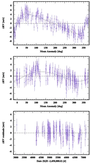
Fig. 1. Left column: From top to bottom, HARPS RV measurements as a function of barycentric Julian Date obtained for HD 20003, HD 20781, HD 21693, HD 31527, HD 45184, HD 51608, HD 134060 and HD 136352. Error bars only include photon and calibration noise. Middle column: log(R0
Table 4. Parameters probed by the MCMC. The symbols U and N used for the priors definition stands for uniform and normal distributions, respectively.
Parameters Units Priors Description Range
Parameters probed by MCMC without magnetic cycle
M? [M ] N (M?,0.1) stellar mass (M?can be found in Table 1)
σX [ m s−1] U instrumental jitter of instrument X ]-∞,∞[ σJIT [ m s−1] U stellar jitter (If only one instrument is used, this parameter includes σX) ]-∞,∞[ γX [km/s] U Constant velocity offset of instrument X ]-∞,∞[
lin [ m s−1yr−1] U Linear drift ]-∞,∞[
quad [m2s−2yr−2] U Quadratic drift ]-∞,∞[
log (P) log([days]) U Logarithm of the period [0,∞[ log (K) log([ m s−1]) U Logarithm of the RV semi-amplitude [0,∞[
√
ecos ω - U ]-1,1[
√
esin ω - U ]-1,1[
λ0= M0+ ω [deg] U Mean longitude (M0= mean anomaly) [0,360[ Parameters probed by MCMC with magnetic cycle (in addition to the previous ones, except σJIT LOWand σJIT HIGHthat replace σJIT σJIT LOW [ m s−1] U stellar jitter at the minimum of the magnetic cycle (If only one
instrument is used, this parameter includes σX) ]-∞,∞[ σJIT HIGH [ m s−1] U stellar jitter at the maximum of the magnetic cycle (If only one
instrument is used, this parameter includes σX) ]-∞,∞[ log(R0
HK) lin [ m s
−1] U slope of the correlation between the RV and log(R0
HK) (The log(R 0
HK) variation
is normalized between 0 and 1, thus this parameter is in [ m s−1]) ]-∞,∞[ Physical Parameters derived from the MCMC posteriors (not probed)
P [d] - Period
K [m s−1] - RV semi-amplitude e - - Orbit eccentricity ω [deg] - Argument of periastron TP [d] - Time of passage at periastron TC [d] - Time of transit
Ar [AU] - Semi-major axis of the relative orbit M.sin i [MJup] - Mass relative to Jupiter
M.sin i [MEarth] - Mass relative the Earth
the GLS periodogram of the calcium activity index log(R0HK), we fit the RVs with a polynomial up to the second order, plus a Keplerian model reproducing the log(R0HK) variation, leaving only the amplitude as a free parameter. Note that when correct-ing magnetic cycle effect in RVs when adoptcorrect-ing a step-by-step approach, we do not consider a simple linear correlation between RV and log(R0
HK) as explained above because significant
plane-tary signals not yet removed from the data might destroy any existing correlation. There is no a priori reason why the mag-netic cycle should look like a Keplerian, however a Keplerien has more degrees of freedom than a simple sinusoid and can there-fore better estimate the long-term variation seen in log(R0HK). Regarding signal significance, a signal is considered worth look-ing into when its p-value, which gives the probability that the signal appears just by chance, is smaller or equal to a chosen threshold. Experience has shown us that a p-value of 1 % pro-vides a good empirical threshold. Note that in this paper, p-values are estimated in a Monte Carlo approach by bootstrapping 10’000 times over the dates of the observations.
4.2. Detection of periodic signals in the data
– Planetary signals are searched for in the GLS periodogram of the RV residuals after correcting long-term trends. As for magnetic cycles, we consider a signal as significant if its
p-value is smaller than 1 %4. If the p-values of some signals in the GLS periodogram are smaller than 1%, we adjust a Ke-plerian orbital solution to the signal presenting the smallest p-value following the approach of Delisle et al. (2016) with the detected period as a guess value.
– Additional planets in the systems are then considered if other significant signals are present in the GLS periodogram of the RV residuals. Note that each time a Keplerian signal is added to the model, a global fit including all the previously detected signals is performed.
– We stopped when no more signals in the residuals present a p-value smaller than 1 % and we finally visually inspected the solutions.
4.3. Origin of the different signals found
After the main periodic signals have been recognized in the data, it is important to identify the ones that are very likely not from planetary origin. They may be of different natures: stellar, in-strumental or observational. Here is a brief description of some cases encountered:
4 The goal of our program is to derive reliable statistical distributions of orbital and planet properties that can be used to constrain planet for-mation models. Signals of less significance are of course of great inter-est but require more observations to be confirmed as bona fide planets.
– Stellar origin. The signal is due to stellar intrinsic phenom-ena. The most common one is the variation of the measured RVs due to spectral line asymmetries induced by spots and faculae coming in and out of view on the surface of the star, modulating the signal over a star rotational period (Hay-wood et al. 2016, 2014; Dumusque et al. 2014a; Meunier et al. 2010; Desort et al. 2007; Santos et al. 2000; Saar & Donahue 1997). In order to recognize RV variations of in-trinsic stellar origin, we compare the periods of the derived orbital solutions with the rotational periods of the stars and their harmonics estimated using the log(R0HK) average activ-ity level (see Table 1, Mamajek & Hillenbrand 2008; Noyes et al. 1984). We also compare the orbital periods with the variation timescales of spectroscopic activity indicators de-rived from the CCF, such as the BIS and the FWHM, and derived from spectral lines sensitive to activity, such as the Ca II H and K lines (S-index and log(R0HK)) or the Hα line (Hα-index).
– Instrumental origin. As already mentioned earlier, spurious signals of small amplitudes with periods close to one year or one of its harmonics (half a year, a third of a year) can be created by a discontinuity in the wavelength calibration in-troduced by the stitching of the detector. The 4k×4kHARPS
CCD is composed of 32 blocks of 512×1024 pixels. When each block were imprinted to form the detector mosaic, the technology at the time was not precise enough to ensure that pixels between blocks had the same size than intra-pixels. Therefore, every 512 pixels in the spectral direction, the CCD presents pixels that differs in size (Wilken et al. 2010). Block stitching may introduce a residual signal in the RVs at periods close to 6 months or 1 year when strong stellar lines crosse block stitchings due to the yearly motion of the Earth around the Sun. As mentioned in Sect. 3, in order to miti-gate this effect new sets of RVs for the stars presented in this paper have been obtained by removing from the correlation masks used the spectral lines potentially affected. For each star, the systemic velocity will shift the stellar spectrum on the CCD, therefore an optimization of the correlation mask is done on a star-by-star basis (for more information, see Du-musque et al. 2015).
– Observational limitations. Aliases have to be taken into ac-count. The ones due to one year or one day sampling effects are well known (e.g., Dawson & Fabrycky 2010). They apply on all signals and not only on the planetary ones.
5. Description and analysis of individual systems
In this section, we present eight planetary systems includ-ing Neptune-mass and super-Earth planets. Presence of planets around these stars and preliminary system characterizations have been announced at the "Extreme Solar System II" conference held at Grand Teton USA in September 2011 and published in Mayor et al. (2011). We present here the detailed analysis of each system with updated data, describing and discussing the derived planetary system characteristics, as well as other (i.e. non-planetary) signals in the data.
5.1.HD20003: Eccentric, close-in Neptune-mass planets close to the 3:1 commensurability
5.1.1. Radial velocity analysis
An ensemble of 184 high signal-to-noise observations (<S/N> of 110 at 550 nm) of HD 20003 have been gathered covering about
11 years (4063 days). The typical photon-noise plus calibration uncertainty of the observations is 0.74 ms−1, well below the
ob-served dispersion of the RVs at 5.35 m s−1. The RVs with their
GLS periodogram and the log(R0HK) time-series are displayed in Fig. 1. A long-period variation is observed in the RV data, as well as in log(R0HK), indicative of a magnetic cycle effect on the ve-locities. To correct the velocities for this effect, we modeled the long-term variation by a Keplerian with parameters fixed and de-termined from the log(R0
HK), except for the amplitude that was
left free to vary.
After correction for the long-period variation due to the magnetic cycle plus fitting a second-order polynomial drift, two peaks very clearly emerge in the periodogram well above the 0.1 % p-value limit, at periods around 11.9 and 33.9 days (Fig. 2). Once those two signals are fitted for along with the mag-netic cycle and the second-order polynomial drift, a significant signal at 184 days appears in the GLS periodogram of the RV residuals, with strong aliases at 127 and 359 days. A global fit including a second-order polynomial drift, a Keplerian for the magnetic cycle and three Keplerians for signals at 11.9, 33.9 and 184 days allows us to model all the variations seen in the RVs. No significant signal (with p-values smaller than 5 %) are then present in the RV residuals (Fig. 2, bottom-right plot).
After this preliminary phase looking for significant signals in the data, we searched for the best-fit parameters with an MCMC, using a model composed of a second-order polynomial drift, a linear correlation of the RVs with log(R0
HK) to adjust the
mag-netic cycle effect, three Keplerians to fit for the signals at 11.9, 33.9 and 184 days, and two jitters that correspond to the in-strumental plus stellar noise at the minimum and maximum of the magnetic cycle (see Sec. 4). This model converged to a sta-ble solution. However, a significant signal in the residuals was still present near 3000 days (Fig. 3), a period similar to the one of the magnetic cycle, an indication that our modeling of the long period variation was not satisfactory, very probably because the magnetic cycle ofHD20003 is not fully covered, as seen in Fig. 1. We finally decided then to adjust a model composed of 3 Keplerians at 11.9, 33.9 and 184 days, an extra Keplerian at long-period to absorb the effect of the magnetic signal plus any long-term trend that could be present in the data, and one jit-ter corresponding to the instrumental plus stellar noise. In this case, the GLS periodogram of the residuals is extremely similar to the last plot in Fig. 2 and therefore no more significant sig-nal is present in those RV residuals. Note that the period of the signal adjusting the magnetic cycle changed however from 4038 days (log(R0HK)) to 3298 days (RVs). Although we do not under-stand fully the long-term signal present in the RVs ofHD20003, adjusting it with different models gives similar orbital parame-ters for the signals at 11.9, 33.9 and 184 days. We adopted as final solution the model with the magnetic cycle modeled by a long-period Keplerian with free parameters.
The best-fit for each inner planet, the signal at 184 days, and the RV residuals are displayed in Fig. 4. The best-fit parameters can be found in Table 5. A careful look at the activity indica-tors, log(R0
HK), BIS SPAN and FWHM, after removing the
long-period signal induced by the stellar magnetic cycle, reveals no significant peaks that match the planetary signals found in our analysis (see Fig. A.1). We are therefore confident that those sig-nals are not induced by stellar activity.
The correlation between the activity index log(R0
HK) and the
RV residuals when removing all the detected signals except the magnetic cycle effect can be seen in the left panel of Fig. 5. Note that this dependence in activity is included in our model when adjusting the long-period Keplerian.
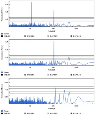
Fig. 2. GLS Periodogram of the RV residuals of HD 20003 at each step after removing, from top-left to bottom-right, the magnetic cycle effect plus a second-order polynomial drift, then the two planets at 11 and 33 days one after the other, and finally the signal at 184 days. The GLS periodogram of the raw RVs is shown in Fig. 1.
Table 5. Best-derived solution for the planetary system orbiting HD20003. For each parameter, the median of the posterior distribution is consid-ered, with error bars computed from the MCMC chains using a 68.3% confidence interval. σO−Ccorresponds to the weighted standard deviation of the residuals around this best solution. All the parameters probed by the MCMC can be found in Annex, in Table B.1
Param. Units HD20003b HD20003c HD20003d? magn. cycle
P [d] 11.8482+0.0016−0.0017 33.9239+0.0239−0.0266 183.6225+1.0051−1.1057 4037.7931+329.9338−231.0018 K [m s−1] 3.84+0.20−0.21 3.15+0.22−0.20 1.62+0.20−0.20 5.72+0.32−0.31 e 0.36+0.05−0.05 0.10+0.08−0.07 0.13+0.11−0.09 0.06+0.06−0.04 ω [deg] -92.74+8.52−8.61 53.33+45.86−34.56 52.14+55.14−56.21 -113.61+75.59−54.68 TP [d] 55489.5110+0.2090−0.2095 55493.2516+4.4223−3.2265 55426.5836+26.7344−27.4821 52787.4615+1011.0883−899.1487 TC [d] 55483.7622+0.3768−0.3634 55496.2240+0.7332−0.8117 55442.1924+5.3361−5.5073 54968.5034+60.5529−61.9929 Ar [AU] 0.0974+0.0034−0.0039 0.1964+0.0068−0.0078 0.6053+0.0213−0.0239 4.7592+0.3033−0.2678 M.sin i [MJup] 0.0367+0.0033−0.0033 0.0454+0.0046−0.0044 0.0406+0.0060−0.0058 0.4093+0.0421−0.0388 M.sin i [MEarth] 11.66+1.04−1.06 14.44+1.47−1.39 12.91+1.91−1.84 130.08+13.40−12.32 γHARPS [m s−1] -16104.1107+0.3698−0.2826 σ(O−C) [m s−1] 1.65 log (Post) -364.1867+3.3177−3.7161
Fig. 3. GLS Periodogram of the RV residuals of HD 20003 obtained from the MCMC solution including a linear correlation between RV and log(R0
HK) to account for the magnetic cycle, a second-order polynomial drift and three Keplerian.
5.1.2. A 3rd planet with a period of 184 days?
Although the signals at 11.9 and 33.9 days are clearly induced by planets orbiting around HD 20003, the signal at 184 days is
more difficult to interpret as it is very close to half a year, with strong aliases at 127 days and 359 days (close to 1/3 and 1 year). As explained in Sec. 4.3, signals at a year or harmonics of it can be induced by a discontinuity in the wavelength calibration introduced by tiny gaps between the different quadrants of the detector. However, the RV data that we analyze here have been corrected for this effect following the work of Dumusque et al. (2015). This correction has been already applied to the RVs of several stars, and has always been successful in removing the spurious signal. The fact that the RV residuals after removing the two planets, and the long-period effect of the magnetic cy-cle do not correlate with the barycentric Earth velocity (BERV, see right panel of Fig. 5) disfavors the hypothesis that the 184-day signal is due to a discontinuity in the wavelength calibration introduced by tiny gaps between the different quadrants of the detector. In conclusion, we would be inclined to claim that this signal at 184 days is a real planetary signal. However, although
Fig. 4. Phase-folded RV measurements of HD 20003 with the best Keplerian solution represented as a black curve for each of the signals in the data. From top-left to bottom-right: planet b, planet c and the signal at 184 days. The residuals around the solution are displayed in the lower-right panel. Contrarily to Fig. 1 error bars include now the instrumental+ stellar jitter from the MCMC modeling. Corresponding planetary orbital elements are listed in Table 5.
Fig. 5. Left: Activity index log(R0
HK) as a function of the RV residuals when removing all the detected signals except the magnetic cycle effect for HD 20003. The observed correlation indicates that most of the RV residual variation is due to activity-related effects. Right: Barycentric Earth velocity projected on the line of sight (BERV) as a function of the RV residuals around the best derived solution without considering the 184-day signal. The fact that no correlation can be observed disfavours the hypothesis that the 184-day signal is due to a discontinuity in the wavelength calibration introduced by tiny gaps between the different quadrants of the detector.
intensively tested, there is always the possibility that the data re-duction system does not correct for all the instrumental effects in this particular case. We leave the signal as a potential one, and encourage other teams to confirm it using other pipelines or other facilities thanHARPS.
5.1.3. Discussion of the planetary system
A surprising aspect of this system is the high eccentricity of the inner planet, e=0.38, while the planet at 33.9 days has an
eccen-tricity close to 0. From a planet formation or a dynamical point of view, this is not straightforward to explain. There might be ac-tually several possibilities to explain the observed configuration. It is out of the scope if this paper to check all of them in details, we just mention here the basic ideas.
1) The first and simplest possibility is that the high eccen-tricity of the planet at 11.9 days actually hides a planet at half the orbital period (Anglada-Escudé et al. 2010), in (or close to) a 2:1 resonance configuration. We therefore tried to fit a model with an extra planet with initial period at 5.95 days, setting the
eccentricities of the 5.95 and 11.9-day planets to zero or letting them free to vary. Model comparison shows that, in both cases, the more complex solution is disfavoured with a∆BIC of 8.3 and 24.3, respectively. It seems therefore that the significant eccen-tricity of planet b is real.
2) The two planets are close to the 3:1 resonance. An in-crease of the eccentricity could have happened if, in the past, the two planets have been migrating trapped in the resonance. Then a specific event made the two planets go slightly out of reso-nance on the nowadays observed orbits. Possible scenarios for this event could be instability when the gas disappeared or the presence of an additional planet (e.g. resonant chain) that was ejected when the eccentricity increased (scattering).
3) Invoking additional bodies in the system raises the possi-bility of an external companion that could induce a Kozai-lidov effect on the inner planets in case of a large mutual inclination (Kozai 1962; Lidov 1961). Such a companion could actually be hinted by our difficulty of modelling the long-period variation observed in the radial velocities. It is however not very clear to understand the differential effect on the two inner planets.
4) Finally, a very appealing potential explanation might rely on the spin-orbit evolution of planets feeling the tidal effect of the central star and the gravitational perturbation of another planetary companion. Correia et al. (2012) have shown that "un-der some particular initial conditions, orbital and spin evolution cannot be dissociated and counter-intuitive behaviors can be ob-served, such as the secular increase of the eccentricity. This ef-fect can last over long timescales and may explain the high ec-centricities observed for moderate close-in planets".
5.2.HD20781: A packed system with 2 super-Earths and 2 Neptune-mass planets
HD 20781 is part of a visual binary system including another star, HD 20782, known to host a planet on a 595-day very eccen-tric orbit (Jones et al. 2006). We take the opportunity of the dis-covery of a compact system of small planets around HD 20781 to provide here as well an updated solution for the planet around HD 20782 usingHARPSdata.
5.2.1. Analysis of theHD20781 system
HD 20781 was part of the original high-precision HARPS GTO survey and the star has been then followed for more than 11 years (4093 days). Over this time span, we gathered a total of 226 high signal-to-noise spectra (<S/N> of 112 at 550 nm) correspond-ing in the end to 216 RV measurements binned over 1 hour. As reported in Table 2, the typical precision of individual measure-ments is 0.76 m s−1including photon noise and calibration
un-certainties. The raw RV rms is significantly higher, at 3.41 m s−1, pointing towards additional variations in the data of potentially stellar or planetary origin, assuming the instrumental effects are kept below the photon-noise level of the observations.
As a first approach we looked at the RV and activity index time series shown in Fig. 1. No significant long-term variation is observed in log(R0HK) data and no long-term variation is visible in the GLS periodogram of the velocity time series. We conclude that there is no noticeable sign of a magnetic activity cycle for this star. The average value of log(R0HK) at −5.03 ± 0.01 is also very low with a very small dispersion, similar to the Sun at min-imum activity.
Due to the small activity level and the large number of ob-servations, the GLS periodogram of the velocity series is very
clean, with significant peaks clearly coming out of the noise background. So, even if the final characterization of the plane-tary system parameters is performed through a Bayesian-based MCMC approach, a step-by-step analysis of the system, charac-terizing and then removing one planet after the other from the data, will provide an excellent illustration of the significance of the planet detection in this system. The most prominent peak in the GLS periodogram is at a period around 20 days. Deriving a Keplerian solution for this planet and then removing the corre-sponding signal from the raw RVs makes a clear signal at 86 days appear in the GLS periodogram of the residuals (Fig. 6). Keeping on with the same approach, we can clearly identify, sequentially, significant signals first at 13.9 and then at 5.3 days. It has to be noted here that none of the significant periods in the data are close to the stellar rotational period, 46.8 days, estimated from the activity index (Table 1).
As described in Sec. 4, the final determination of the plan-etary system parameters is performed using a MCMC sampler and a model composed of four Keplerians representing the plan-etary signals, and an extra white-noise jitter to consider potential stellar or instrumental noise not included in the RV error bars (the σJIT parameter, see Table 4). Phase-folded planetary
solu-tions, as well as the RV residuals around the best solution, are displayed in Fig. 7. The best-fit parameters are reported in Ta-ble 6.
Looking at the periodograms of the log(R0HK), the BIS SPAN and the FWHM in Fig. A.2, to check if any announced planet matches any signal in the activity indicators, we see that the log(R0
HK) times series presents signals at 115, 81 and 68 days,
and the FWHM time series at 380 days. This later signal is prob-ably due to interaction with the window functions, creating a signal near a year. The former signals are more difficult to in-terpret as they are not compatible with the estimated rotational period of the star, 46.8 days (Table 1). In particular, we can note that the 86-day Neptune-mass planet has a period close to the detected peaks in the log(R0
HK) time-series at 81 days, and
fur-thermore is close to the 1-year alias of the 115-d signal (days). The amplitude of these signals however very low, at the level of ∼0.01 dex, 20 times smaller than the solar magnetic cycle varia-tion. Such signals can therefore probably not be responsible for the 2.6 m s−1periodic variation detected in the RVs at 86 days.
Our conclusion is thus that the system HD 20781 hosts two inner super-Earths with periods of 5.3 and 13.9 days and two outer Neptune-mass planets with periods of 29 and 86 days. With small eccentricities, stability is not a concern for this system of small-mass planets in a moderately compact configuration. 5.2.2.HD20782: More planets in this visual binary system The star HD 20782 is the brightest companion of the HD 20781-HD 20782 binary system. It is known to harbor a 595-day very eccentric Jupiter planet (Jones et al. 2006). A total of 71 high signal-to-noise spectra (<S/N> of 181 at 550 nm) were obtained withHARPSon this target, which translates into 68 RV measure-ments after binning the data over 1 hour. Because of the very large semi-amplitude and eccentricity of the RV signal induced by the planet, we decided to include in addition to theHARPS
very precise measurements the lower precision RV data obtained with UCLES (published in Jones et al. 2006) andCORALIE.
We searched for the best-fit parameters using a MCMC sam-pler. The solution converges to an extremely eccentric Jupiter-mass planet with a period of 597 days. The phase-folded plane-tary solution, as well as the RV residuals around the best solution and their GLS periodogram, are displayed in Fig. 8. The best-fit
Fig. 6. GLS periodogram of the residuals at each step, after removing one planet after the other in the analysis of HD 20781 (from left to right and top to bottom). The GLS periodogram of the raw RVs is shown in Fig. 1.
Fig. 7. Phase-folded RV measurements of HD 20781 with the best-fit solution represented as a black curve for each of the signal found in the data (from left to right and top to bottom: planet b, c, d and e). Error bars include photon and calibration noise, as well as instrumental+ stellar jitters derived from the MCMC modeling. The residuals around the solution are displayed in the lower panel. Corresponding orbital elements are listed in Table 6.
parameters are reported in Table 6. Although the eccentricity, the amplitude and the argument of periastron are compatible within one sigma with the values presented in Jones et al. (2006), the period and argument of periastron are not compatible, even if different by less than 2%. This can be explained by the addition
of the CORALIE andHARPS data that allows to sample much better the periastron passage.
The high eccentricity of HD 20782 b has commonly been explained via the Kozai-Lidov mechanism (Kozai 1962; Lidov 1961) induced by HD 20781.
Table 6. Best-fitted solution for the planetary system orbiting HD 20781 and HD 20782. For each parameter, the median of the posterior distribution is considered, with error bars computed from the MCMC posteriors using a 68.3 % confidence interval. The value σ(O−C) corresponds to the weighted standard deviation of the residuals around the best solution. All the parameters probed by the MCMC can be found in Annex, in Tables B.2 and B.3. See Table 4 for definition of the parameters.
Param. Units HD20781b HD20781c HD20781d HD20781e HD20782b
P [d] 5.3135+0.0010−0.0010 13.8905+0.0033−0.0034 29.1580+0.0102−0.0100 85.5073+0.0983−0.0947 597.0643+0.0256−0.0256 K [m s−1] 0.91+0.15−0.15 1.81−0.16+0.16 2.82+0.17−0.16 2.60+0.14−0.14 118.43+1.78−1.78 e 0.10+0.11−0.07 0.09+0.09−0.06 0.11+0.05−0.06 0.06+0.06−0.04 0.95+0.001−0.001 ω [deg] 84.04+141.70−108.41 7.44+53.87−70.21 60.99+30.79−30.03 70.59+61.40−67.58 143.58+0.56−0.66 TP [d] 55503.2027+2.0979−1.5934 55503.5204+2.0425−2.6815 55511.3258+2.4394−2.4382 55513.3912+14.3623−16.0090 55247.0150+0.0770−0.0837 TC [d] 55503.2888+0.2361−0.2384 55506.4386+0.3546−0.4385 55513.2432+0.4250−0.4410 55517.4714+1.3596−1.4838 55246.1712+0.0706−0.0706 Ar [AU] 0.0529+0.0024−0.0027 0.1004+0.0046−0.0051 0.1647+0.0076−0.0083 0.3374+0.0155−0.0170 1.3649+0.0466−0.0495 M.sin i [MJup] 0.0061+0.0012−0.0011 0.0168−0.0021+0.0022 0.0334+0.0038−0.0037 0.0442+0.0049−0.0049 1.4878+0.1045−0.1066 M.sin i [MEarth] 1.93+0.39−0.36 5.33−0.67+0.70 10.61+1.20−1.19 14.03+1.56−1.56 472.83+33.22−33.88 offsetUCLES [m s−1] 5.4431+0.9302−0.9370 γCOR98 [m s−1] 39928.1039+1.8747−1.9160 γCOR07 [m s−1] 39930.6146+2.0828−2.1696 γCOR14 [m s−1] 39956.5569+1.5850−1.6638 γHARPS [m s−1] 40369.2080+0.1147−0.1104 39964.8070+0.2193−0.2275 σ(O−C) [m s−1] 1.45 2.34 log (Post) -397.1395+3.0943−3.8525 -379.6596+2.6521−3.2805
Fig. 8. Best keplerian solution for the eccentric planet orbiting HD 20782. Top: Phase-folded RV measurements with the best solution represented as a black curve. Bottom: RV residuals around the best Ke-plerian solution.
5.3.HD21693: A system of 2 Neptune-mass planets close to a 5:2 resonance
Over a time span of 11 years (4106 days), 212 high signal-to-noise spectra (<S/N> of 141 at 550 nm) of HD 21693 were gath-ered, resulting in a total of 210 RV measurements when bin-ning the data over 1 hour. The typical photon-noise and calibra-tion uncertainty is 0.60 m s−1, which is significantly below the
4.72 m s−1observed dispersion of the RVs, pointing towards the existence of additional signals in the data. The raw RVs, their GLS periodogram and the calcium activity index of HD 21693 are shown in Fig. 1. The variation of the log(R0
HK) ranging from
-5.02 to -4.83 highlights a significant magnetic cycle. This mag-netic cycle is very similar in magnitude to the one of the Sun, but slightly shorter with a period of 10 years. When fitting a Keple-rian signal to the log(R0HK), we are left with significant signals in the residuals at 740 and 33.5 days (see Fig. A.3). Those sig-nals are also present in the FWHM and the bisector span of the CCF, although less significant. The signal at ∼740 days, close to two years is probably due to the sampling of the data, and the 33.5-day signal is likely the stellar rotation period. This value is compatible with the rotation period derived from the mean activ-ity log(R0
HK) level, i.e. 36 days (Table 1).
Looking at the raw RVs and their GLS periodogram in Fig. 1, it is clear that the observed magnetic cycle has an impact on the measured RV measurements. To remove the RV contribution of the magnetic cycle, we remove from the RVs a Keplerian model that has the same parameters as the Keplerian fitted to log(R0HK) but with an amplitude free to vary. The GLS periodogram of the
Fig. 9. Top: GLS periodogram of the residual RVs of HD 21693 after removing the RV contribution of the magnetic cycle. Middle and bot-tom: GLS periodogram of the residuals at each step, after removing one planet after the other in the analysis. The GLS periodogram of the raw RVs is shown in Fig. 1.
RV residuals after correcting for the magnetic cycle effect are displayed in the top panel of Fig. 9. A highly significant signal at 54 days is present in the data. When removing this signal by fit-ting a Keplerian, an extra signal at 23 days is seen in the residuals (middle panel of Fig. 9). No signal with p-value smaller than 1 % appears in the residuals of a two-Keplerian model; we therefore stop looking for extra signals. Note however that the most signif-icant signal left in the GLS periodogram corresponds to a period of 16 days, likely the first harmonic of the stellar rotation period, which is expected from stellar activity (Boisse et al. 2011).
After this preliminary phase looking for significant signals in the data, we search for the best-fit parameters with an MCMC, using a model composed of a linear correlation of the RVs with log(R0
HK) to adjust the magnetic cycle effect, two Keplerian
func-tions for the signals at 23 and 54 days, and two jitter values cor-respond to the instrumental plus stellar noise at the minimum and maximum of the magnetic cycle (see Sec. 4). The best-fit for each planet and the RV residuals are displayed in Fig. 10, and the best-fit parameters can be found in Table 7. None of the two detected planet corresponds to signals found in the activity indi-cators (see Fig. A.3).
When looking at the RV residuals, the scatter is still rather high even after removing all the significant signal detected in the data. Although in Hipparcos the star is catalogued as a G8 dwarf, the spectroscopic survey of nearby stars NSTAR finds that that HD 21693 is a G9IV-V therefore a slightly evolved star (Gray et al. 2006). Evolved stars presents higher photometric and RV jitter associated with more significant granulation, which might explain this significant residual jitter (Bastien et al. 2014, 2013; Dumusque et al. 2011c).
The correlation between the activity index log(R0HK) and the RV residuals removing only the two-planet solution can be seen in Fig. 11. Note that this correlation is considered in the MCMC model we used to fit the RV data.
Our analysis of theHARPSRV measurements of HD 21693 provides strong evidence that 2 Neptune-mass planets orbit the star, with periods of 22.7 and 53.7 days. With such periods, this planetary system is close to a 5:2 resonance but with a period ra-tio smaller than the 5:2 commensurability. If the system formed through a convergent migration scenario trapping the planets in the 5:2 resonance, some process has to be invoked to push the system out of the resonance configuration after the disappear-ance of the protoplanetary disk.
Fig. 10. Phase-folded RV measurements of HD 21693 with the best planet solution represented as a black curve for each of the signal in the data (top to bottom: planet b and planet c). The residuals around the solution are displayed in the lower panel. Corresponding orbital el-ements are listed in Table 7.
5.4.HD31527: A 3-Neptune system
In total, 257 high signal-to-noise spectra (<S/N> of 180 at 550 nm) of HD 31527 were gathered over a time span of 11 years (4135 days). This results in 245 observations of the star when data are binned over 1 hour. The 3.19 m s−1observed dis-persion of the RVs is much larger than the typical RV preci-sion of 0.64 m s−1, pointing towards the existence of extra
sig-nals in the data. The raw RVs, their GLS periodogram and the calcium activity index of HD 31527 are shown in Fig. 1. The calcium activity index log(R0HK) does not show any significant variation as a function of time, therefore we do not expect the
Fig. 11. RV residuals when removing all the detected signals except the magnetic cycle effect plotted as a function of the activity index log(R0
HK) for HD 21693. The observed correlation indicates that most of the RV residual variation is due to activity-related effects.
Table 7. Best-fitted solution for the planetary system orbiting HD 21693. For each parameter, the median of the posterior is consid-ered, with error bars computed from the MCMC chains using a 68.3 % confidence interval. σO−Ccorresponds to the weighted standard devia-tion of the residuals around this best soludevia-tions. All the parameters probe by the MCMC can be found in Annex, in Table B.4.
Param. Units HD21693b HD21693c P [d] 22.6786+0.0085−0.0087 53.7357+0.0312−0.0309 K [m s−1] 2.20+0.22−0.22 3.44+0.20−0.20 e 0.12+0.09−0.08 0.07+0.06−0.05 ω [deg] -91.04+50.57−50.35 -17.34+47.50−55.35 TP [d] 55492.0549+3.0968−3.1310 55528.4064+7.0762−8.1820 TC [d] 55480.7554+0.7454−0.6973 55543.5822+1.0676−1.2491 Ar [AU] 0.1455+0.0058−0.0063 0.2586+0.0103−0.0113 M.sin i [MJup] 0.0259+0.0034−0.0033 0.0547+0.0056−0.0056 M.sin i [MEarth] 8.23+1.08−1.05 17.37+1.77−1.79 γHARPS [m s−1] 39768.8113+0.1425−0.1471 σ(O−C) [m s−1] 2.05 log (Post) -440.9160+2.2958−3.1188
RVs to be affected by long-period signals generally induced by magnetic cycles. The mean activity level of the star is equal to log(R0HK)= −4.96, close to solar minimum. The RVs should therefore be exempt as well of activity signal at the rotational period of the star and its harmonics due to active regions on the stellar surface (Boisse et al. 2011). This is confirmed when looking at the periodograms of the different activity indicators in Fig. A.4. Only a signal at 400 days in the BIS SPAN is
sig-nificant. This signal, not too far from a year, might be due the interplay between the time series and the window function.
Fig. 12. Top: GLS periodogram of the residual RVs of HD 31527 after removing the best-fit Keplerian to account for the significant signal at 17 days seen in the raw RVs (bottom right panel of Fig. 1). Middle and bottom: GLS periodogram of the residuals at each step, after removing the second and third planet from the RVs.
As we can see in the GLS periodogram of the raw RVs (Fig. 1), two extremely significant signals appear at 17 and 52 days. After fitting these signals with a two-Keplerian model, a third significant signal at 271 days can be seen in the RV resid-uals (middle panel of Fig. 12). Finally, the residresid-uals of a three-Keplerian model do not show any signal with p-value smaller than 1 % (bottom panel of Fig. 12). The fact that no signal is present at the estimated rotation period of the star (19 days, Ta-ble 1) or its harmonics confirms that the RVs of HD 31527 are not affected by significant activity signal.
After this first search for significant signals in the data, we fitted, using a MCMC sampler, a three-Keplerian model to the data including a white-noise jitter component to account for stel-lar and instrumental uncertainties not included in the RV error bars. The best-fit for each planet, as well as the RV residuals, can be seen in Fig. 13. We report in addition the best-fit parame-ters in Table 8.
None of the signals announced here matches signals in the different activity indicators (see Fig. A.4).We therefore conclude that HD 31527 hosts 3 Neptune-mass planets, with periods of 16.6, 51.2 and 272 days. The star is a G2 dwarf like the Sun, therefore the outer planet in this system lies on an orbit between the ones of Venus and the Earth, therefore in the habitable zone of its host star (Selsis et al. 2007). This planet, with a minimum mass of 13 Earth-masses, is however most likely composed of a large gas envelope (Rogers 2015; Wolfgang & Lopez 2015; Weiss & Marcy 2014), except if it is similar to Kepler-10 c in composition (Dumusque et al. 2014b).
Fig. 13. Phase-folded RV measurements of HD 31527 with the best Keplerian solution for planet b, c, d and e represented as black curves (from left to right and top to bottom). Error bars include photon and calibration noise, as well as a jitter estimated from the MCMC analysis. The residuals around the solution are displayed in the bottom right panel. Corresponding orbital elements are listed in Table 8.
Table 8. Best-fitted solution for the planetary system orbiting HD 31527. For each parameter, the median of the posterior distribution is considered, with error bars computed from the MCMC chains using a 68.3 % confidence interval. σO−Ccorresponds to the weighted standard deviation of the residuals around the best solution. All the parameters probeb by the MCMC can be found in Annex, in Table B.5.
Param. Units HD31527b HD31527c HD31527d P [d] 16.5535+0.0034−0.0035 51.2053+0.0373−0.0368 271.6737+2.1135−2.2471 K [m s−1] 2.72+0.13 −0.13 2.51+0.14−0.14 1.25+0.17−0.16 e 0.10+0.05−0.05 0.04+0.05−0.03 0.24+0.13−0.13 ω [deg] 41.12+29.46−34.41 -23.25+68.94−152.43 179.00+31.11−26.20 TP [d] 55499.5453+1.3130−1.5818 55526.3434+9.7876−21.5943 55718.8091+21.3880−17.3759 TC [d] 55501.4585+0.2640−0.2667 55542.0635+0.7471−0.9373 55670.8324+11.7715−13.7509 Ar [AU] 0.1254+0.0041−0.0045 0.2663+0.0088−0.0095 0.8098+0.0273−0.0293 M.sin i [MJup] 0.0329+0.0028−0.0028 0.0445+0.0040−0.0039 0.0372+0.0053−0.0052 M.sin i [MEarth] 10.47+0.89−0.87 14.16+1.28−1.23 11.82+1.70−1.64 γHARPS [m s−1] 25739.7025+0.0952−0.0971 σ(O−C) [m s−1] 1.41 log (Post) -439.4138+2.7350−3.3929
5.5.HD45184: A system of two close-in Neptunes
We gathered a total of 309 high signal-to-noise spectra (<S/N> of 221 at 550 nm) of the G1.5 dwarf HD 45184 during a time span of 11 years (4160 days). This results in 178 RV measure-ments, when the data are binned over 1 hour. The average pre-cision of the RVs is 0.41 m s−1 considering only photon noise and calibration uncertainties. The raw RV rms is much higher, 4.72 m s−1, which implies that significant signals are present in the data. In Fig. 1, we display the raw RVs and their GLS
pe-riodogram, and the log(R0HK) time series. We see that a signifi-cant magnetic cycle affects log(R0
HK), with values ranging from
-5.00 to -4.86 with a periodicity of 5 years. This magnetic cycle is therefore smaller in amplitude and period than the solar cy-cle, despite the similarities of the derived stellar parameters with those of the Sun. To see if significant signals were present in the calcium activity index despite the long-period magnetic cycle, we fitted the log(R0HK) time series with a Keplerian. In the resid-uals, a strong signal at 20 days is present, likely corresponding
Fig. 14. From top to bottom: GLS periodogram of the RVs after remov-ing the effect induced by the stellar magnetic cycles and then one planet after the other in the analysis of HD 45184. The GLS periodogram of the raw RVs is shown in Fig. 1.
to the stellar rotation period (see Fig. A.5). This value is fully compatible with the rotation estimated using the log(R0HK) aver-age level (21.5 days, see Table 1; Mamajek & Hillenbrand 2008; Noyes et al. 1984).
Looking at the raw RVs of HD 45184 and their GLS peri-odogram in Fig. 1, we see that the magnetic cycle observed in log(R0
HK) has an influence on the RVs. To remove the RV
con-tribution of the magnetic cycle, we fitted the log(R0HK) with a Keplerian, and removed the same Keplerian from the RVs leav-ing the amplitude as a free parameter. In the residuals, displayed in the top panel of Fig. 14, we see a significant signal at 6 days. Once this signal is removed by fitting a Keplerian with the cor-responding period, another signal at 13 days appears (see middle panel of Fig. 14). Finally after removing a two-Keplerian model to the RVs corrected for the magnetic cycle effect, no signal with p-value smaller than 10 % remains. We therefore stop looking for extra signals in the data. Note that although not significant, the highest peak in the GLS periodogram of the RV residuals is at 18.6 days, likely the imprint of the stellar rotation period. The RVs are therefore slightly affected by stellar activity, however at a level that is not perturbing the detection and characterization of the two planets at 6 and 13 days.
After the preliminary phase of looking for significant sig-nals, we fitted the RVs using a MCMC sampler and a model composed of a linear correlation of the RVs with log(R0
HK) to
adjust the magnetic cycle effect, two Keplerians to fit for the sig-nals at 5.9 and 13.1 days, and two jitters that correspond to the instrumental plus stellar noise at the minimum and maximum of the magnetic cycle (see Sec. 4). Each planet with its best fit can be seen in Fig. 15, as well as the RV residuals after the best solution has been removed. The best-fit parameters are reported in Table 9. None of the signals at 5.9 and 13.1 matched signals in the different activity indicators (see Fig. A.5), and therefore those signal are associated with bona-fide planets.
Fig. 15. Phase-folded RV measurements of HD 45184 with, from top to bottom, the best Keplerian solution for planets b and c, and the corre-sponding residuals. Error bars include photon and calibration noise, as well as a jitter effect (stellar + instrumental) determined in the MCMC analysis. Corresponding orbital elements are listed in Table 9.
In Fig. 16, we show the RV residuals after removing the best-fit solution for planets b and c as a function of the log(R0HK). The observed strong correlation indicates that most of the residuals are due to activity-related effects and motivates the use of our model that includes a correlation between log(R0
HK) and RVs to
mitigate the effect of long-term activity.
5.6.HD51608: 2 Neptune-mass planets
Over a time span of 11 years (4158 days), 218 high signal-to-noise spectra (<S/N> of 133 at 550 nm) of HD 51608 were gathered withHARPS, resulting in a total of 216 measurements binned over 1 hour with a typical photon-noise and calibration uncertainty of 0.62 m s−1. This value is significantly below the observed 4.07 m s−1dispersion of the RVs, pointing towards the
existence of additional signals in the data. The raw RVs, their GLS periodogram and the calcium activity index of HD 51608 are shown in Fig. 1. A small, albeit significant, long-term varia-tion can be seen in log(R0HK), with values in log(R0HK) ranging from -5.04 to -4.96 and with a period of 11 years. Although the period of this magnetic cycle is very similar to that of the Sun, its amplitude is much lower. After fitting this long-period