HAL Id: hal-00317546
https://hal.archives-ouvertes.fr/hal-00317546
Submitted on 7 Sep 2004
HAL is a multi-disciplinary open access
archive for the deposit and dissemination of
sci-entific research documents, whether they are
pub-lished or not. The documents may come from
teaching and research institutions in France or
abroad, or from public or private research centers.
L’archive ouverte pluridisciplinaire HAL, est
destinée au dépôt et à la diffusion de documents
scientifiques de niveau recherche, publiés ou non,
émanant des établissements d’enseignement et de
recherche français ou étrangers, des laboratoires
publics ou privés.
Middle Atmosphere Model (FUB-CMAM) to different
gravity-wave drag parameterisations
P. Mieth, J. L. Grenfell, U. Langematz, M. Kunze
To cite this version:
P. Mieth, J. L. Grenfell, U. Langematz, M. Kunze. Sensitivity of the Freie Universität Berlin Climate
Middle Atmosphere Model (FUB-CMAM) to different gravity-wave drag parameterisations. Annales
Geophysicae, European Geosciences Union, 2004, 22 (8), pp.2693-2713. �hal-00317546�
Sensitivity of the Freie Universit¨at Berlin Climate Middle
Atmosphere Model (FUB-CMAM) to different gravity-wave drag
parameterisations
P. Mieth1,2, J. L. Grenfell2, U. Langematz2, and M. Kunze2
1Deutsches Zentrum f¨ur Luft- und Raumfahrt, Institut f¨ur Verkehrsforschung, Rutherfordstr. 2, 12489 Berlin, Germany 2Institut f¨ur Meteorologie, Freie Universit¨at Berlin, Carl-Heinrich-Becker-Weg 6–10, 12165 Berlin, Germany
Received: 29 September 2003 – Revised: 5 April 2004 – Accepted: 5 May 2004 – Published: 7 September 2004
Abstract. We report the sensitivity of the Berlin Climate
Middle Atmosphere Model (CMAM) to different gravity-wave (GW) parameterisations. We perform five perpetual January experiments: 1) Rayleigh friction (RF) (control), 2) non-orographic GWs, 3) orographic GWs, 4) orographic and non-orographic GWs with no background stress, and 5) as for 4) but with background stress. We also repeat exper-iment 4) but for July conditions. Our main aim is to im-prove the model climatology by introducing orographic and non-orographic parameterisations and to investigate the in-dividual effect of these schemes in the Berlin CMAM. We compare with an RF control to determine the improvement upon a previously-published model version employing RF. Results are broadly similar to previously-published works. The runs having both orographic and non-orographic GWs produce a statistically-significant warming of 4–8 K in the wintertime polar lower stratosphere. These runs also fea-ture a cooling of the warm summer pole in the mesosphere by 10–15 K, more in line with observations. This is asso-ciated with the non-orographic GW scheme. This scheme is also associated with a heating feature in the winter po-lar upper stratosphere directly below the peak GW-breaking region. The runs with both orographic and non-orographic GWs feature a statistically-significant deceleration in the po-lar night jet (PNJ) of 10–20 ms−1in the lower stratosphere. Both orographic and non-orographic GWs individually pro-duce some latitudinal tilting of the polar jet with height, although the main effect comes from the non-orographic waves. The resulting degree of tilt, although improved, is nevertheless still weaker than that observed. Accordingly, wintertime variability in the zonal mean wind, which peaks at the edge of the vortex, tends to maximise too far polewards in the model compared with observations. Gravity-planetary wave interaction leads to a decrease in the amplitudes of sta-tionary planetary waves 1 and 2 by up to 50% in the
up-Correspondence to: J. L. Grenfell
per stratosphere and mesosphere, more in line with obser-vations. Comparing modelled and observed Eliassen-Palm fluxes suggests that planetary wave (PW) breaking occurs too far polewards in the model. The wind and temperature changes are consistent with changes in the Brewer-Dobson (BD) circulation. Results suggest that the effect of enforcing a minimum background wave stress in the McFarlane scheme could be potentially important. In the Southern Hemisphere (SH) in July, the GW schemes had only a small impact on the high-latitude lower stratosphere but there featured strong warming near 0.1 hPa.
Key words. Meteorology and atmospheric dynamics;
Gen-eral circulation; Middle atmosphere dynamics; Waves and tides
1 Introduction
Correctly parameterising the sub-grid-scale effects of grav-ity waves (GWs) remains a major challenge for the present-day hierarchy of general circulation models (GCMs). GWs are transverse oscillations with typical length scales of 10–1000 km in the horizontal, 1–100 km in the vertical and typical lifetimes of the order of hours. They arise when air parcels in a stably-stratified atmosphere undergo a vertical displacement and subsequently experience a restoring buoy-ancy force. Fritts (1984) and McLandress (1998) provide a good overview. Orographic excitation has long been recog-nised (e.g. Long, 1953). Non-orographic sources, for exam-ple, wind shear (Lindzen and Rosenthal, 1976), convection and weather fronts (Clarke et al., 1986) and geostrophic ad-justment (Fritts and Luo, 1992) have been investigated.
GWs are believed to represent an important mechanism for mixing and carry momentum upwards from the tropo-sphere. When GWs saturate and break this results in an en-ergy cascade to smaller scales, turbulent diffusion, and de-position of momentum. Wave dissipation leads to the zonal
mean force necessary to balance the Coriolis torque which ultimately drives the meridional circulation when air parcels cross surfaces of constant angular momentum. This force stimulates the reversed temperature gradient of the sum-mer to winter circulation in the mesosphere, which effects displacement away from radiative equilibrium (McIntyre, 2001) and also produces drag which decelerates and tends to close off the top of the middle atmosphere (MA) jet. In the lower stratosphere, downward control implies enhanced downward motion in the wintertime vortex, on incorporat-ing GW schemes (Hines, 1991) which produces a warmincorporat-ing effect. GWs are also believed to play a role in forcing the quasi-biennial oscillation (QBO) (Dunkerton, 1997; Scaife et al., 2000; Giorgetta et al., 2002).
The development of GW parameterisations in atmospheric models has received wide attention in recent years. Most conclude that there has been an improvement in the cold pole problem due to GW stimulation of the Brewer-Dobson (BD) circulation, hence enhanced subsidence in the polar night jet (PNJ) (Rind et al., 1988; Garcia and Boville, 1994; Beagley et al., 2000). Some studies note the difficulty of choosing appropriate tuning parameters and find that the cold pole, though weaker, still persists (Rozanov et al., 2001). Norton and Thuburn (1997) report that a scheme originally based on Lindzen (1981) better reproduces the observed equatorward tilt of the polar night jet.
Various works compare different GW schemes and per-form sensitivity studies with the tuning parameters. Jack-son (1993) notes that a positive phase-speed, c=20ms−1 (rather than c=0) for non-orographic waves, greatly enables more waves to propagate through the summer mesosphere and leads to an improved easterly wind simulation, whereas the c=0 waves are absorbed mainly near the extra-tropical tropopause. Lawrence (1997) compares the Hines scheme with the Fritts/Luo non-orographic scheme and finds that the former scheme reproduces a more realistic PNJ with better variability. Manzini and McFarlane (1998) report that tem-perature in the lower and upper stratosphere of their GCM is sensitive to the launch height of their GW spectrum. Char-ron et al. (2002) compared the Hines scheme with a scheme of Warner and McIntyre (WM), which differed mainly in that the latter employed an empirically-derived expression for wave-dissipation. That work found similar mesospheric wave forcings only when the lower stratosphere momentum fluxes were an order of magnitude lower for WM than Hines. New orographic schemes have recently emerged (Lott and Miller, 1997; Gregory et al., 1998; Scinocca and McFarlane, 2000), which suggest that flow blocking and internal wave reflection may be important.
It is generally accepted that GW parameterisations may profoundly influence the meridional circulation, hence tem-perature and zonal mean zonal wind in the GCMs. How-ever, a particular scheme does not always produce similar results when implemented in different models. This is be-cause GCMs differ in how they resolve dynamical processes such as planetary wave excitation in the troposphere. Hence GW schemes employ model-dependent tuning parameters to
reduce remaining biases. Such parameters, however, cannot address biases not related to the GWs. They are used to esti-mate initial launch characteristics, wave-flow interaction and momentum deposition fluxes. GW schemes suffer from a lack of seasonality and regionality in their source spectra due to a paucity of observational data.
Some studies utilise observations to constrain their GW parameterisations. Broad (1996) employed vertical velocity aircraft data and finds good agreement at night but under-estimation during the morning which that author attributes to the process of boundary layer ascent initiating GWs not rep-resented in the model. Alternatively, hydroxyl (OH) band emission intensity measured by radar can be used to esti-mate GW amplitude, period and phase-speed (Takahashi et al., 1998). Ongoing international projects, such as the Strato-spheric Processes and their Role in Climate (SPARC) GW climatology project (Allen and Vincent, 1995), play a vital role in this regard by compiling reliable global data cover-age of GW activity and seasonality. Finally, it is interest-ing to note that although the grids of most GCMs are too coarse explicitly to resolve GWs, some short time scale, high-resolution studies claim to have achieved this for the larger GWs (Sato et al., 1999; Hamilton et al., 1999).
In the present study, we perform five sensitivity experi-ments with differing gravity-wave parameterisations imple-mented in the Freie Universit¨at Berlin Climate Middle Atmo-sphere Model (FUB CMAM). We estimate the GW momen-tum flux, examine the response of the meridional circulation, discuss the impact upon the “cold pole” problem, the zonal mean zonal wind, the wintertime rates of mean descent in the PNJ and the influence upon stationary and transient planetary waves (PWs). Section 2 provides a model description and overview of the experiments; Sect. 3 presents results; Sect. 4 provides the discussion, conclusions and future work.
2 Model and experimental setup
2.1 Model description
The model is described in Langematz and Pawson (1997) and Pawson et al. (1998). Its dynamical core solves the primi-tive equations based on the so-called spectral representation (Baede et al., 1979). We employ a triangular truncation (T21) where “21” is the maximum number of waves resolved in the meridional or zonal direction and corresponds to a grid-scale of ∼5.6×5.6◦. There are 34 levels in the vertical which
extend from the ground up to ∼84 km. Near the surface a terrain-following sigma coordinate is employed, which re-laxes toward isobaric surfaces on the upper layers, the so-called “hybrid” system (Simmons and Str¨ufing, 1983). A de-tailed treatment of the hydrological cycle is incorporated, in-cluding prognostic clouds, deep and shallow convection and surface exchange (Roeckner et al., 1992). Shortwave heat-ing is based on Fouquart and Bonnel (1980) with the addi-tion of solar absorpaddi-tion by O3and O2above 70 hPa using the
fer (Langematz, 2000) eliminated the warm polar bias of the previous model version. Climatological ozone fields are em-ployed, updated from Fortuin and Langematz (1994). Av-eraged (1979–1991) sea-surface temperatures based on the Atmospheric Modelling Intercomparison Project (AMIP) are employed to avoid the bias of sampling a particular phase of El Ni˜no. Long-lived greenhouse gases (GHGs) other than CO2(uniformly set to 330 ppmv ) are not included. The
var-ious GW schemes are described separately below. 2.2 Overview of runs
The original motivation for including GWs was to address the model’s underestimation of subsidence in the PNJ, the strong jet and the cold pole, as was apparent in a previous annual cycle run with full online chemistry (not shown). A series of test runs (presented here) were accordingly conceived, without online chemistry, to test the effect of orographic and non-orographic GW parameterisations in the model. The response of GCMs to such schemes has already been documented in other models. Nevertheless, this procedure was a necessary part of our model development. This work broadly confirms the generally-accepted response to the GW schemes in the Berlin CMAM. Due to limited computer resources, the test runs are performed in perpetual January/July mode, although naturally, it would have been preferable to perform multi-year runs with a full annual cycle. All runs are of fifteen months in duration, with the first four months discarded for spinup purposes.
Experiment 1: Control (Rayleigh friction)
Rayleigh friction (RF) entails a linear relaxation of the zonal and meridional components, e.g. u=uold+(du/dt), and
(du/dt)=−Ku, where the constant K corresponds approx-imately to time scales of 2.5 day−1 at 83 km, 5 day−1 at 76 km, 10 day−1at 73 km and 25 day−1at 69 km (so-called RF “sponge layers”) (Holton and Wehrbein, 1980). Long integrations of the model, which also employed Rayleigh friction have been documented (e.g. Langematz and Pawson, 1997); hence, we adopt this parameterisation as our control for this study. Although RF is effective at exponentially damping over-strong winds, its drawbacks are that it violates momentum conservation and tends to produce thermally-driven cells, inconsistent with the concept of the mechanically-driven meridional circulation (Shepherd, 2000). RF always drags the winds back to zero, artificially lowering variability, whereas observed winds may go to zero and then often change direction (Kim et al., 2003). On the other hand, RF is easy to implement and effectively closes off the polar jet in the model upper layers. With these caveats in mind, the RF run employed coefficients such that only a weak drag was exerted in the mesosphere without impacting the stratosphere and without influencing PW
Non-orographic gravity-waves redistribute momentum within the atmosphere (whereas orographic waves exchange momentum between the solid Earth and the atmosphere). These differing conceptual frameworks should be kept in mind when comparing different experiments. Non-orographic GW drag (Hines, 1991; 1997) is implemented in a coding after Manzini and McFarlane (1998). The scheme assumes an initial, vertical spectral density proportional to mx, where “m” is the vertical wave number and “x” is an integer. For this study we adopt “x” equal to 1 with a launch height close to the surface. The launch spectrum is isotropic and time-invariant and is characterised by a launch slope of 1 (vertically upward), σhorizontalwind=1.5 ms−1,
and horizontal wave number=7×10⁻⁶m−1. Manzini and McFarlane (1998) provide further details. As the waves propagate upward, their amplitudes increase exponentially in response to the decrease in gas density. The scheme imposes height-dependent Doppler spreading in the frequency dis-tribution, which parameterises wave-wave interaction, and Doppler shifting of the mode frequency, which parameterises wave-mean-flow interaction. Wave breaking is imposed using a cut-off criterion, with value:
m = N( V-Vo+φ1σ +φ2σtot)−1,
where m = vertical cut-off wave number N = Brunt V¨ais¨all¨a frequency
V = horizontal windspeed Vo = windspeed at launch height
σ =variability of horizontal wind arising from GW
σtot= variability of total horizontal wind
φ1, φ2 are tunable parameters which represent the
wave-wave interaction and the wave-wave-mean-flow interaction, respectively. For our runs we adopt φ1=1.5 and φ2=0.3
which corresponds to the middle range of recommended values (Hines, 1991; Hines, 1997). Waves having wave-lengths greater than the above “cut-off” value are assumed to be saturated. The cut-off value is derived from empirical evidence and is a function of N and σtot (Hines, 1997).
Once saturated, momentum deposition (MD) is calculated according to MD=hP(m(z))−1, where h=horizontal wave number, P=horizontal wind power spectrum, m(z)=vertical wave number, constrained such that MD is positive and increasing with height.
Medvedev and Klaassen (2000) note a caveat of the Hines scheme, namely it does not produce the characteristic (m−3)
dependency in the power spectrum, (m=vertical wave num-ber) found in observations (Smith et al., 1987). This differ-ence is attributed to the instantaneous “chopping” of waves above the “cut-off” saturation value, whereas in the real at-mosphere, saturation continually adjusts to changes in, for example, temperature and density as the waves propagate up-wards and wave-breaking is a more gradual process in time and space.
Experiment 3: orographic GWs (McFarlane scheme), background = on
The scheme is described in McFarlane (1987). The coding for our study is adapted from the Community Climate Model (CCM) version 3.6 (Boville, 1995). “background=on” im-plies that a small, latitude-dependent background stress is utilised in all regions whenever the orographic stress is smaller than a minimum background value (NCAR tech-nical note NCAR/TN-417+STR, 1996). This reflects the model’s underestimation of weak wave stresses and is a rather crude way of parameterising subscale processes. Mo-mentum is not conserved but is added to the system at low wave stresses. Numerically, the background stresses τ(back)
parameterise orographic variation in a simple way such that: (NH):τ(back)=τ(N H )*sin(2*latitude) τ(N H )=0.75 ms−2,
SH:τ(back)=τ(SH )*sin(2*latitude) τ(SH )=1.2 ms−2. Turning
on the background switch forces the surface wave stresses always to be greater than a minimum background value. So, like RF, the background switch is effect-driven, not process-driven and does not conserve momentum.
The initial wave momentum flux, M, at a particular oro-graphic height is taken to be:
M = − ( Eµm2/2)ρNV,
where E= efficiency factor (<1; a function of orographic height)
µ= horizontal wave number m = horizontal amplitude
ρ =gas density
N = Brunt V¨ais¨all¨a frequency
V = wind component in direction of flow,
where the wave amplitude fulfilled the condition: m = min(2σorog,FcU/N),
where σorog= standard deviation of sub-grid-scale orography
(assumed isotropic)
Fc= critical Froude number (F2c=0.5)
U = zonal wind.
All waves having local F>Fcare assumed to be saturated.
So, the waves could break when the convective instability cri-terion is satisfied, i.e. the vertical gradient of total potential temperature becomes negative. The equations above show that the orographic wave momentum flux is directly related to the standard deviation of the orography. This study used orography data obtained from the United States Navy high resolution data set with resolution 10×10 arc min (Cuming and Hawkins, 1981), corresponding to about 20×20 km. A new, higher-resolution data set with a resolution of approx-imately 1×1 km has been recently reported (Webster et al., 2003). The orographic scheme always assumes F2c=0.5 and horizontal wavelength=100 km. Radiative damping is ap-plied in the vertical with a Newtonian cooling coefficient, α =1×10⁻⁶ s−1. Only stationary waves are considered. Experiment 4: Hines and McFarlane combined, background = off
Experiment 5: Hines and McFarlane combined, background = on
3 Results
3.1 January runs
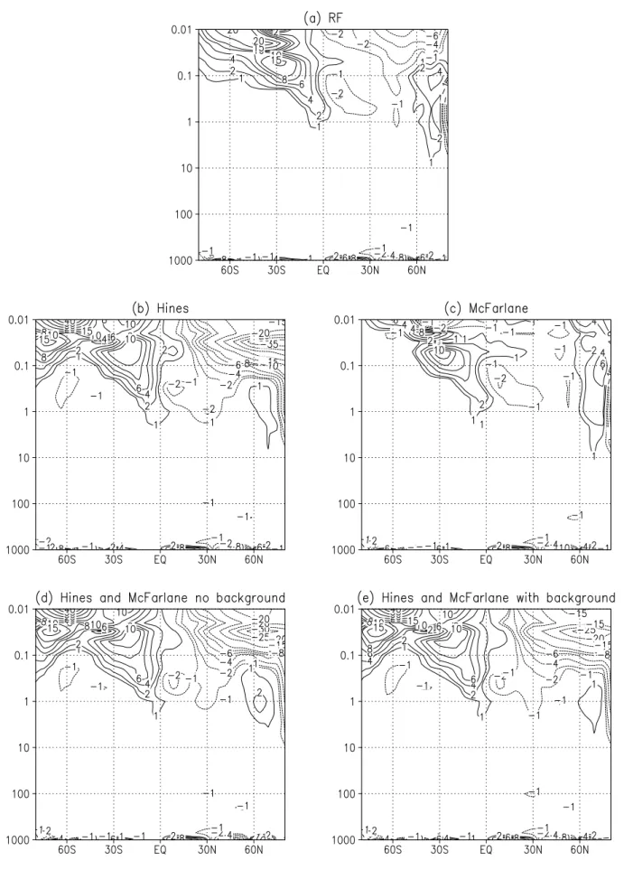
Figure 1a shows observed January zonal mean zonal wind (u) data taken from the Stratospheric Processes and their Role in Climate (SPARC) Intercomparison of Middle Atmosphere Climatologies Report (2002). The data covers the period 1992–1997 and is a composite of the United Kingdom Mete-orological Office (UKMO) analyses (Swinbank and O’Neill, 1994) and the High Resolution Doppler Imager (HRDI) data sets (Hays et al., 1993). Figures 1b–f show umodelfor
experi-ments 1–5. Figures 2a–d show (umodel-uRF)for experiments
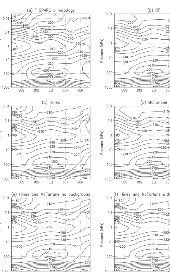
2–5 respectively. Figures 3a–f are the same as Figs. 1a–f but for temperature (T). Likewise, Figs. 4a–d are the same as Figs. 2a–d but for T. The observed temperatures are also taken from SPARC (2002) and cover the period 1992–1997. They are a composite of the UKMO analyses, the Halogen Occultation Experiment (HALOE) (Russell et al., 1993) and the Microwave Limb Sounder (MLS) (Fishbein et al., 1996) data sets.
The RF run displays an over-strong, over-cold PNJ in the lower stratosphere, having too little equatorward tilt with increasing altitude and too high summer temperatures in the polar mesosphere (Figs. 1b, 3b). Although the oro-graphic GWs (experiment 3) produce some equatorward tilt in the jet in the upper stratosphere (Fig. 1d), the main ef-fect comes from the non-orographic waves (experiment 2, Fig. 1c). Manzini et al. (1997) note broadly similar improve-ments on comparing the same non-orographic scheme with an RF scheme in the MA. Including both orographic and non-orographic waves is necessary to produce a statistically-significant deceleration of 10–20 ms−1 in the PNJ in the
lower stratosphere from 50 to 10 hPa (Figs. 2c, 2d). The im-posed GW drag also weakens the over-strong summertime easterlies, more in line with observations. Compare, for ex-ample u in the control run (Fig. 1b) with u in the runs having both types of GWs (Figs. 1e, 1f), in which the easterlies are weakened by around 10% at 50–60◦S, 0.1 hPa. The top of the easterly jet is also closed more realistically on the upper layers in the GW runs. The sub-tropical jets are mostly unaf-fected. The model does not simulate the QBO in the tropical mid stratosphere (a well-known bias in MA GCMs using RF parameterisations) (Pawson, 1992) but instead features weak easterlies throughout the year. M¨uller et al. (1997) and Nis-sen et al. (2000) studied the semiannual oscillation (SAO) in a previous model version of the FUB CMAM without GWs. Results implied the modelled easterlies were sometimes too strong by 10–15 m/s compared with observations.
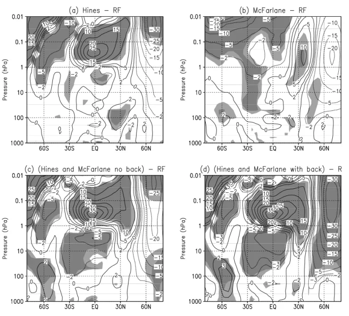
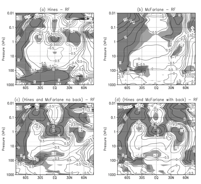
Separately, the non-orographic and orographic schemes lead to a 2–4 K warming of the cold pole in the wintertime lower stratosphere (Figures 4a, 4b, respectively). This quan-tity is approximately doubled when both schemes operate to-gether (Figs. 4c, 4d). The orographic waves alone (Fig. 4b) are associated with a statistically-significant warming in the lower stratosphere (+4 K at 100 hPa, 70◦N) at high lati-tudes, whereas the non-orographic waves alone (Fig. 4a)
Fig. 1. January mean zonal mean zonal wind in ms−1for (a) observations (SPARC climatology), (b) Rayleigh friction, (c) Hines non-orographic scheme, (d) McFarlane non-orographic scheme, (e) both (c) and (d), background drag off (f) as for (e) but with background term on.
Fig. 2. January mean zonal mean wind difference in ms−1for (a) Hines minus RF, (b) McFarlane minus RF, (c) Hines and McFarlane (background off) minus RF, (d) Hines and McFarlane (background on) minus RF. Light grey shading denotes the 95% confidence interval and dark grey shading denotes the 99% confidence interval calculated from the t-distribution. Contour values for (a) to (c): −30, −25, −20, −15, −10, −5, −2, 0, 2, 5, 10, 15, 20, 25, 30, 35. Contour values for (d): −30, −25, −20, −15, −10, −5, −3, −2, 0, 2, 3, 5, 10, 15, 20, 25, 30, 35.
have a stronger impact on higher levels, (+10 K, 0.7–0.3 hPa, 70◦N). Furthermore, the desired cooling of 10–15 K in the summertime polar mesosphere is associated purely with the non-orographic scheme (Figs. 4b–d) and not the oro-graphic scheme (Fig. 4a), which actually produces some heating in this region, implying that the orographic scheme has a weaker effect on the upper levels compared with RF. The non-orographic runs also feature statistically-significant heating in the tropical upper stratosphere, the NH mid-latitude mesosphere and the SH high-mid-latitude lower strato-sphere. We show later that these temperature changes are consistent with the response of the Brewer Dobson circula-tion to the imposed drag from the breaking GWs.
Figure 5 compares model results (output at the equator) for January for the various experiments with rocketsonde
obser-vations (M¨uller et al., 1997) (shown as a plain line). Above 1 hPa easterly tropical winds in the RF run (crosses) are too strong by 10–15 ms−1compared with the observations. In-cluding the GWs improves the situation considerably; in the upper stratosphere the effect is mainly associated with the Hines scheme alone (open circles).
We have compared model variability with that calculated by the UKMO (United Kingdom Meteorological Office) database, which encompasses 1992–2000 data with a lid at 0.3 hPa. Figures 6a–f are as for Figs. 1a–f but show one standard-deviation of u. We have also calculated similar plots but using NCEP CPC (National Centers for Environmen-tal Prediction Climate Prediction Center) data (not shown), which encompass the years 1979–1998 and which feature a lid at 1.0 hPa. Results from both data sets are reasonably
Fig. 4. As for Fig. 2, but for temperature in K. Contour values −10, −8, −6, −4, −2, −1, −0.5, 0, 0.5, 1, 2, 4, 6, 10.
similar, although the UKMO features higher values around 10mb in the tropics compared with the NCEP CPC. This may be linked, on the one hand, with the shorter measuring period of the UKMO data set. On the other hand, the NCEP CPC dataset, like other reanalysis data sets, suffers from a paucity of sampling in the tropics (Waliser et al., 1999) and tends to underestimate the QBO.
Figure 6 suggests that the RF scheme (experiment 1) cap-tures u variability reasonably well, except in the tropics where it underestimates. This arises because the model lacks a QBO (but there are also caveats with the data here, as al-ready discussed). For all runs, peak variabilities in zonal mean wind tend to occur too far polewards. Related to this, the vortex edge (i.e. the region of peak wind variability) lacks latitudinal tilt with height. This is a typical GCM problem, as already discussed. All GW experiments tend to increase peak u variability in Fig. 6, except run 5 (Hines and Mc-Farlane, background drag on), where it decreases slightly. Increasedvariability results from the direct influence of the
breaking GWs upon the zonal mean zonal wind. Decreased variability, as it occurred in run 5, has also been documented in some other works. This arises at least partly via the rather subtle interaction of GWs with planetary waves (PWs), in which the latter may either strengthen (Manzini and Mc-Farlane, 1998; Smith, 1997) or weaken (Miyahara et al., 1986), depending on whether phase-speeds and orientations favour constructive or destructive interference with the GWs. McLandress and McFarlane (1993) provide an overview of GW and PW interaction. The nature of the interaction de-pends upon adjustable factors, such as GW launch height and directionality. Manzini and McFarlane (1998), for ex-ample, noted that moving from the surface to the tropopause favours enhanced PW weakening. Also, including horizon-tal variability in the GW spectrum (such as in the orographic scheme) tends to favour PW generation; removing it leads to the opposite effect (McLandress and McFarlane, 1993). A further contribution to the decrease in variability in run 5 (Hines and McFarlane, back on) could be the switching on of
RF 207.98 − 19.14 − 223.98 − 3.90 −
Hines 212.00 +1.93 34.84 +82.03 225.13 +0.51 4.74 +21.54
McFarlane 216.16 +3.93 29.98 +56.64 224.20 +0.10 3.44 −11.79 both+back 213.59 +2.70 36.62 +91.33 223.75 −0.10 4.24 +8.72 both-back 219.12 +5.36 22.34 +16.72 224.03 +0.02 2.46 −36.92
Fig. 5. Modelled zonal mean zonal wind (m/s−1) output at the equator for the January experiments. The rocketsonde observa-tions are also shown here as a plain line. RF run (cross); Hines run (open circle); McFarlane run (closed circle); Hines and McFarlane background off (open square); Hines and McFarlane background on (closed square).
background drag in this run. This tends to lower variability by constraining GW stresses to always be higher than a small background value, which is independent of latitude and lon-gitude and is applied immediately after the calculation of the GW stresses.
Table 1 shows January mean temperature (K) on 10 hPa and its 2-sigma variability for the various experiments at the North Pole (NP) and at 60◦N. Percent changes are relative to the RF run. Internal model variability in this region of the atmosphere is an indicator of the model’s ability to simu-late sudden stratospheric warmings. Table 1 shows that GWs have a larger impact at the NP, producing up to 11.3 K heat-ing and are associated with a large increase in variability. As
already discussed for u-variability, the effect of switching on background drag is associated with a suppression in the vari-ability. At 60◦N the GWs have a much smaller impact com-pared with the NP, as already illustrated in Fig. 4. The ab-solute changes at 60◦N are much smaller (up to 0.5%) than at the NP and the variability changes range from −36.9 to +21.5%. Again, switching on the background drag reduces the variability, at 60◦N to such an extent that it becomes lower than in the control run. Zonal mean temperature plots of observed (UKMO) and modelled temperature variability (not shown) supported the results in Table 1, namely that variability increased rapidly from 60◦N to the pole, peak-ing around 3 hPa in both model and observations. Interest-ingly, the model predicted a secondary peak over the pole at 0.1 hPa, in a region above the lid of the UKMO database, near where GW breaking occurred (as we show later). Why does the stratospheric T-variability peak over the pole? An important factor affecting stratospheric temperature variabil-ity is planetary wave forcing originating in the troposphere (Pawson and Kubitz, 1996). Associated with this, inside the PNJ, air parcels may experience rapid excursions in the verti-cal associated with large changes in adiabatic heating, hence temperature.
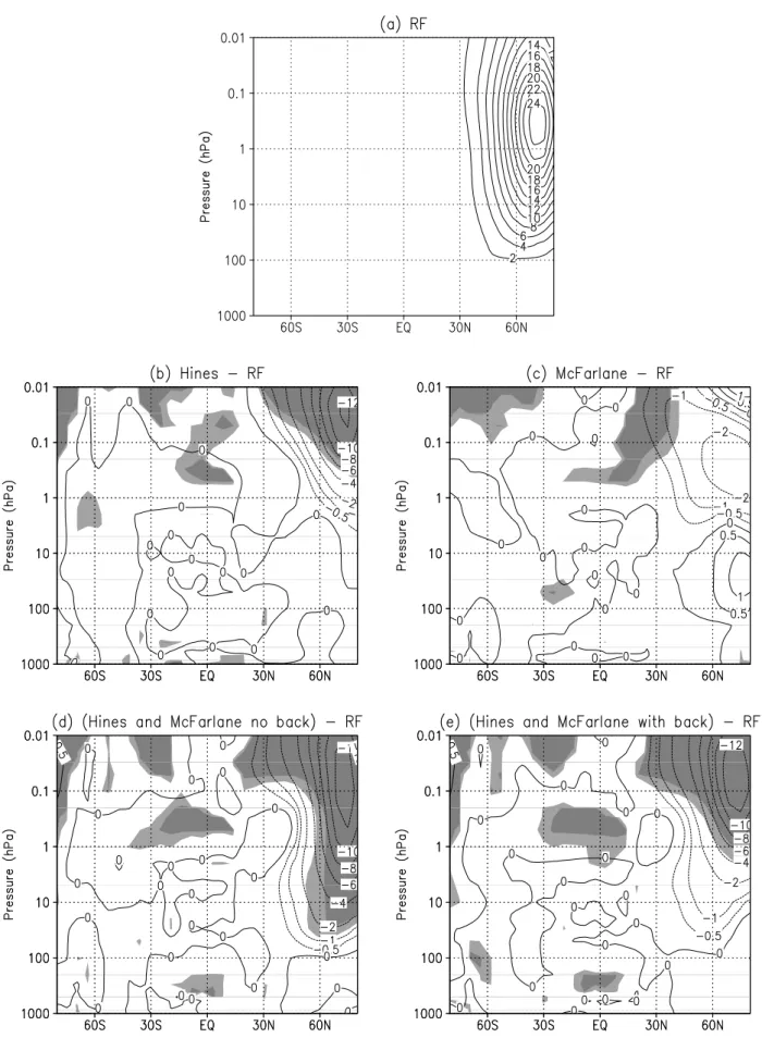
Figure 7a shows the mean amplitude of stationary plane-tary waves of wave number 1 for the RF run. Figures 7b-e show the difference for experiments 2 to 5, respectively. Fig-ures 8a–e is as for Figs. 7a–e but for wave number 2. Quan-tities shown in Figs. 7 and 8 are a measure of standing eddy energy calculated by standard Fourier transform based on an original output interval of 4 h averaged to one month. Ran-del (1992) has published a stationary PW climatology (not shown) in which the amplitude of wave number 1 peaks at 900 m close to 3 mb, 65◦N, whereas wave number 2 peaks
at 200 m close to 50 mb, 65◦N. By comparison in the RF run (Figs. 7a, 8a) the modelled waves peak at higher altitudes and feature higher values. The latter partly reflects a resolution problem. The cold pole problem is also related, which im-plies an over-stable vortex hence a bias towards stationary waves 1 and 2. Note that the GW tunable parameters are not designed to address such resolution issues. Moving to a higher resolution will be the focus of a newly-planned model version.
Fig. 6. January mean standard deviation of the zonal mean zonal wind in ms−1for observations [UKMO] and for experiments 1–5. Contour values are: 1, 2, 5, 10, 15, 20, 25, 30, 35, 40.
Fig. 7. January mean geopotential amplitude in 100m units of stationary wave number one for (a) RF run, (b) Hines minus RF, (c) McFarlane minus RF, (d) Hines and McFarlane background off minus RF, (e) Hines and McFarlane background on minus RF. Contour interval for (a): 2; contour values for (b)–(e): −12, −10, −8, −6, −4, −2, −1, −0.5, 0, 0.5, 1, 2, 4, 6, 8, 10, 12.
Fig. 9. As for Fig. 7 but for gravity wave momentum flux (GWMF) (m/s/day) for experiments 1–5. Contour values: −35, −30, −25, −20,
The non-orographic GWs (Figs. 7b, 8b) decrease quite strongly the amplitudes of wave 1 and wave 2, closer in line with observations. The orographic GWs have a much smaller effect, which is not statistically-significant. It is informative to compare the PW amplitude plots (Figs. 7 and 8) and the u variability plots (Fig. 6). The reduction in wave 1 (e.g. from the control to the non-orographic GW runs, Figs. 7a–b) cor-responds to a reduction in u variability in the wintertime up-per mesosphere (Figs. 6b–c). We do not consider changes in higher order stationary waves. Also, transient waves (consid-ered in the following section discussing EP-fluxes) are also playing a role. Volodin and Schmitz (2001) report that their MA GCM (with the Hines scheme included) underestimates monthly variability and the amplitudes of waves one and two, in contrast to this work. Rind et al. (1988) parameterise oro-graphic and non-orooro-graphic GWs and underestimate station-ary PW wave amplitudes by 20–30%, concluding that Eddy dissipative processes are too strong in their model. A more exhaustive treatment of the nature of such interactions would be better suited to a simpler mechanistic model rather than a GCM, which is beyond the scope of this work.
Similar to the approach of Pawson et al. (1998), GW mo-mentum fluxes may be approximated by assuming that only GWs and PWs exert drag upon the zonal mean wind and then adopting the transformed Eulerian mean (TEM) approach (Andrews et al., 1987):
GW MF = (∂u/∂t ) − (ρ0acos φ)−1∇ ·F − ¯v∗f
+ ¯v∗(acos φ)−1( ¯ucos φ)φ+ ¯w∗u¯z,
where GWMF= GW momentum flux (ms−1day−1);
ρo= surface density;
u, v, w = zonal, meridional and vertical wind vectors in di-rections x, y, z,
a = radius of the Earth;
φ= latitude;
F = Eliassen-Palm-flux vector, f = Coriolis parameter;
¯
uz= vertical derivative of the zonal mean wind,
( ¯ucos φ)φ=horizontal derivative of the zonal mean wind, ¯
v∗= ¯v − ρ−01(ρ0( ¯v0θ¯0)/ ¯θz)z,
¯
w∗= ¯w + (acos φ)−1(cos φ ( ¯v0θ¯0)/ ¯θz)z θ =potential temperature.
GWMF is shown in Figs. 9a–e for experiments 1–5, re-spectively. The main effect comes from the non-orographic waves (Fig. 9b). Values in Fig. 9b compare reasonably well with other model studies, (e.g. Manzini et al., 1997), who studied the Hines scheme, and Manzini and McFar-lane (1998), who studied the Hines and McFarMcFar-lane schemes together. The main differences arise in the SH where our values are up to 50% smaller for runs having both types of GWs. Also, our non-orographic GWMF peak values occur about 10◦further poleward compared with those two studies.
McLandress (1998) noted that GWMF values in the Hines non-orographic scheme almost double when the minimum launch height (currently uncertain) is changed from one-third to two-thirds of a kilometre. GWMF for the RF run com-pares quite well with that of the Hines scheme in the SH, but the RF run has smaller values in the winter mesosphere compared with Hines.
GWMF from the orographic scheme (Fig. 9c) has only a small effect in the Northern Hemisphere (NH). McFarlane and Manzini (1997), calculated GWMF values for the Mc-Farlane scheme from −5 to −15 ms−1peaking near 70◦N, 70 km. Pawson et al. (1998) calculated rather higher values in GWMF for the Palmer orographic scheme (Palmer et al., 1986). Clearly, a climatology based on observations of the quantity GWMF is highly-desirable but this is not currently available.
Figure 10a shows the meridional stream function, an indicator of the BD circulation, for the control run. Figures 10b–e show differences for runs 2 to 5, respectively. Positive values indicate clockwise motion in the plane of the paper and vice-versa. Figures 11a–e are as for Figs. 10a–e but show the transformed mean vertical velocity (Andrews and McIntyre, 1978) for which positive values indicate up-ward motion. For the experiments with non-orographic GWs, the three temperature features noted earlier (i.e. cool-ing in summer mesosphere, warmcool-ing in upper stratosphere tropics and warming in lower stratosphere high latitudes) are all consistent with a strengthening in the BD circulation. Firstly, cooling in the summer mesosphere results from stim-ulated ascent in the upward branch of the SH BD circulation (positive values in Figs. 11b, d, e). Secondly, as air parcels move from the summer to winter hemisphere in the tropics, the streamlines imply descent, hence a stronger BD circula-tion leads to heating here. Thirdly, heating in the NH polar lower stratosphere occurred because this is a region of over-all descent (e.g. Fig. 11b), so again a stronger BD circula-tion leads to heating. The orographic GW run (Figs. 10c, 11c) features, on the other hand, some heating in the summer mesosphere and virtually no tropical heating feature. This result is also consistent with the BD circulation changes in Figs. 10c, 11c, which imply a weakening in the circulation in the summertime mesosphere. Subsidence in the PNJ of the control run (Fig. 11a) is rather weak in the lower strato-sphere. This was one of the original reasons for implement-ing the GW schemes. Introducimplement-ing GWs clearly improves this problem as shown by the negative values in Fig. 11e, imply-ing stimulated descent between 100–10 hPa. Although our region of peak GW breaking is broadly consistent in terms of magnitude and location with other studies already men-tioned, our results imply there is room for further improve-ment in the lower stratosphere. This could reflect a need to increase further the magnitude of the momentum and heat flux from the breaking GWs via the tuning parameters in the model.
Figure 12a shows the monthly-mean EP-flux divergence observations taken from the NCEP CPC (20 years data, lid=1 hPa). Figures 12b shows the same values but for the
Fig. 10. As for Fig. 7 but for the meridional mass stream function in 106kg/s. Positive values indicate clockwise motion in the plane of the paper and vice-versa. Values represent mass flow through a 1 m3volume. Contour values for (a): −600, −400, −200, −100, −50, 0, 10, 30, 50, 100, 300, 500, 1000, 2000, 3000, 4000, 5000; contour values for (b)–(e): −500, −400, −300, −200, −100, −50, −30, −10, 0, 5, 10, 15, 20, 25, 50, 100, 150, 200, 300.
Fig. 11. As for Fig. 7 but for the transformed mean vertical velocity in mms−1. Contour interval for (a): 1.0. Contour values for (b) − (f): −8, −6, −4, −2, −1, −0.5, −0.2, 0.2, 0.5, 1, 2, 3, 4.
Fig. 12. (a) Observed EP flux divergence (ms−1day−1)for NCEP CPC (1979–1998). (b) As for (a) but for the RF run, (c) Hines minus RF (d) McFarlane minus RF, (e) Hines and McFarlane background off, (f) Hines and McFarlane background on. Contour values for (a) and (b):
−30, −20, −10, −8, −6, −4, −2, −1, 1, 2, 4, 6, 8, 10, 20, 30; contour values for (c)−(f): −30, −20, −10, −8, −6, −4, −2, −1, −0.5, 0, 0.5, 1, 2, 4, 6, 8, 10, 20, 30.
Fig. 13. July mean zonal mean zonal wind in ms−1for (a) observations ([SPARC climatology), (b) Hines and McFarlane schemes with background drag off, (c) as for (a) but for temperature (K), and (d) as for (b) but for temperature (K).
RF run. Figures 12c–f show the difference from the RF run for experiments 2 to 5, respectively. EP-flux divergence is a measure of how PWs directly influence the zonal mean flow. A caveat of the comparison is, the calculation of di-vergence for the observations is based on a time interval of 24 h, whereas the model calculation used 4 hours. However, since the inherent time scale of transient planetary waves is of the order of several days; the associated error of this caveat is likely to be small. The comparison shows in the NH the westerly forcing (negative) values tilt polewards with height in the GCM, whereas observations suggest an equatorwards tilt with height. Observed and modelled values are generally comparable in the troposphere. In the stratosphere, the region of maximum activity in the observations is confined to 30– 40◦N whereas the model spreads the high values 30–80◦N.
This may reflect an inability of T21 to adequately capture the smaller PWs. In the upper stratosphere and mesosphere the model experiments were all fairly robust.
3.2 July run
This run was as for experiment 4, i.e. Hines and McFarlane, background off, but for July conditions. Figures 13a–b show zonal mean wind (ms−1)for observations (again the SPARC climatology) and model, respectively. Figures 13b–c show the same but for temperature (K). Only one model month is shown here. Nevertheless, since model variability is quite low in the modelled SH stratosphere (T2σ=1–3 K), and since
the signals we discuss are rather strong, they are likely also to feature in a July climatology. The GWs have a relatively small impact on the high-latitude lower stratosphere. Here, the PNJ remains strong (Fig. 13b) and cold (Fig. 13d), com-pared with the observations, and the tilt of the jet in the model is hardly affected, unlike in the NH. A strong warming in the SH at high-latitudes near 0.1 hPa is also apparent. The results illustrate that care is required when implementing GWs and choosing the tuneable parameters.
have documented the resulting changes in u, T and related these to changes induced by the GWMF in the BD circu-lation. We have also investigated u, T variability and have discussed GW-PW interaction in the model.
Closest correspondence with observations is generally found for those experiments having both orographic and non-orographic waves. Here, the over strong PNJ weakens by 10– 20 ms−1in the MA and the underestimated tilting with height of the jet is somewhat improved. In the upper stratosphere, the Hines scheme leads to a weakening of the tropical easter-lies by 10–15 m/s, more in-line with observations. Including both types of GWs, the cold pole in the lower stratosphere warms by 4–8 K and the warm polar mesosphere in summer cools by 10–15 K. All these changes are related to a strength-ening of the Brewer Dobson circulation. Variability in u, T is best captured in the run with both Hines and McFarlane schemes with background stress on but is otherwise gener-ally overestimated, except in the tropics, where the model lacked a QBO. Stationary wave amplitudes decrease by up to 50% in experiments having both types of GWs, better in line with observations. Despite these clear improvements, in the NH winter lower stratosphere - an important region for ozone chemistry – the results suggest that there is still room for improvement, for example, the cold pole is still not com-pletely eradicated. This may reflect a need to revise the GW tuneable parameters in future.
Clearly, the Hines and McFarlane GW schemes and also the background wave stress switch have the potential to impact strongly the stratospheric dynamics in our GCM. Whether the background parameterisation is sufficiently re-alistic should be the focus of future work. There currently exist major uncertainties in the seasonal, latitudinal and al-titudinal dependence of GW sources and sinks on a global scale. Introduction of the so-called GW tuning parameters represents a first attempt to circumvent this ignorance. Ob-taining climatological, global, observationally-based data to make redundant the tuning parameters is an obvious priority, already underway.
Acknowledgements. We thank E. Manzini for providing the code
for the Hines scheme, the National Center for Atmospheric Re-search (NCAR) for providing the coding for the McFarlane scheme, N. McFarlane for useful discussions and two anonymous referees for their comments. The rocketsonde data was kindly provided by NCAR. PM was supported by the European Union (EU) Project EuroSPICE (European Project on Stratospheric Processes and their Impact on Climate and the Environment), contract number EVK2-CT-1999-00014. JLG was supported by the BMBF (Bundesmin-isterium f¨ur Bildung und Forschung), grant number FKZ-01-SF-9958, as part of the ENVISAT (Environmental Satellite) Project. The GCM simulations were performed at the Konrad-Zuse-Zentrum f¨ur Informationstechnik, Berlin.
Topical Editor O. Boucher thanks two referees for their help in evaluating this paper.
100, 1327–1350, 1995.
Andrews, D. G. and McIntyre, M. E.: Generalized Eliassen-Palm and Charney-Drazin theorems for waves on axisymmetric mean flows in compressible atmospheres, J. Atmos. Sci., 35, 175–185, 1978.
Andrews, D. G., Holton, J. R., and Leovy, C. B.: Middle Atmo-spheric Dynamics, Academic Press Inc. (London) Ltd., 1987. Baede, A. P. M., Jarraud, M., and Cubasch, U.: Adiabatic
formu-lation of ECMWF’s spectral model. ECMWF Tech. Rep., 15, 1– 40, 1979.
Beagley, S. R., McLandress, C., Fomichev, V. I., and Ward, W. E.: The extended Canadian middle atmosphere model, Geophys. Res. Lett., 27 (16), 2529–2532, 2000.
Boville, B. A.: Middle atmosphere version of CCM2 (MACCM2): Annual cycle and interannual variability, J. Geophys. Res., 100, 9017–9039, 1995.
Broad, A. S, High-resolution numerical-model integrations to val-idate gravity-wave parametrization schemes: a case-study, Q. J. R. Meteorol. Soc., 122 (535), 1625–1653, 1996.
Charron, M., Manzini, E., and Warner, C. D.: Intercomparison of gravity wave parameterisations: Hines Doppler-spread and Warner and McIntyre ultra-simple schemes. J. Meteor. Soc. Japan, 80, 335–345, 2002.
Clark, T. E., Hauf, T., and Kuettner, J. P.: Convectively forced in-ternal gravity waves: Results from two-dimensional numerical experiments, Q. J. R. Meteorol. Soc., 112, 899–925, 1986. Cuming, M. J. and Hawkins, B. A.: TERDAT: The FNOC
Sys-tem for Terrain Data Extraction and Processing, Tech. rep. MII Project M254 (Second Edition), Meteorology International In-corporated, 1981.
Dunkerton, T. T.: The role of gravity waves in the quasi-biennial oscillation, J. Geophys. Res., 66, 813–818, 1997.
Fishbein, E., Cofield, R. E., and Froidevaux, L., et al.: Validation of the UARS Microwave Limb Sounder temperature and pressure measurements, J. Geophys. Res., 101, 9983–10 016, 1996. Fortuin J. P. and Langematz, U.: An update on the global ozone
climatology and on concurrent ozone and temperature trends, Proceedings of the International Society for Optical Engineering (SPIE): Atmospheric Sensing and Modelling, 2311, 207–216, 1994.
Fouquart, Y. and Bonnel, B.: Computations of solar heating of the earth’s atmosphere: a new parameterization, Beitr. Phys. Atmos., 53, 35–62, 1980.
Fritts, D. C.: Gravity wave saturation in the middle atmosphere: a review of theory and observations, Revs. Geophys. Spa. Phys., 22 (3), 275–308, 1984.
Fritts, D. C. and Luo, Z.: Gravity wave excitation by geostrophic adjustment of the jet stream, Part 1: Two dimensional forcing, J. Atmos. Sci., 49, 681–697, 1992.
Garcia, R. R. and Boville, B. A.: “Downward control” of the mean meridional circulation and temperature distribution of the polar winter stratosphere, J. Atm. Sci., 51, 2238–2245, 1994. Giorgetta, M., Mancini, E., and Roeckner, E.: Forcing of the
quasi-biennial oscillation from a broad spectrum of atmospheric waves, Geophys. Res. Lett., 29(8), 861–864, 2002.
Gregory, D., Shutts, G. J., and Mitchell, J. R.: A new gravity-wave-drag scheme incorporating anisotropic orography and low-level wave breaking: impact upon the climate of the UK
Meteorolog-ical Office Unified Model, Q. J. R. Meteorol. Soc., 124 (546), 463–493, 1998.
Hamilton, K., Wilson, R. J., and Hemler, R. S.: Middle atmosphere simulated with high vertical and horizontal resolution versions of a GCM: Improvements in the cold pole bias and generation of a QBO-like oscillation in the tropics, J. Atmos. Sci., 15, 56 (22), 3829–3846, 1999.
Haynes, P. H., Marks, C. J., McIntyre, M. E., Shepherd, T. G., and Shine, K. P.: On the “downward control” of extratropical di-abatic circulations by Eddy-induced mean zonal forces, Amer. Met. Soc., 48 (4), 651–678, 1991.
Hays, P. B., Abreu, V. J., and Dobbs, M. E., et al.:The high-resolution Doppler imager on the Upper Atmosphere Research Satellite, J. Geophys. Res., 98, 10 713–10 723, 1993.
Hines, C. O.: The saturation of gravity waves in the middle atmo-sphere. Part I: critique of linear-instability theory, J. Atmos. Sci., 48 (11), 1348–1359, 1991.
Hines, C. O.: Doppler-spread parameterization of gravity-wave mo-mentum deposition in the middle atmosphere. Part 1: Basic for-mulation, J. Atm. Sol-Terr. Phys., 59, 371–386, 1997.
Holton, J. R.: An introduction to dynamical meteorology, third edi-tion, edited by Dmowska, R. and Holton, J. R., Academic Press, San Diego, California, USA, 1992.
Holton, J. R. and W. M. Wehrbein: A numerical model of the zonal mean circulation of the middle atmosphere, Pure Appl. Geo-phys., 130, 41–443, 1980.
Jackson, D. R.: Sensitivity of the extended UGAMP general circu-lation model to the specification of gravity-wave phase speeds, Q. J. R. Meteorol. Soc., 119 (511), 457–468, 1993.
Kim, Y. J., Eckermann, S. D., and Chun, H. Y.: An Overview of the Past, Present and Future of Gravity-Wave Drag Parametrization for Numerical Climate and Weather Prediction Models, Atm.-Ocean, 41(1), 65–98, 2003.
Langematz, U.: An estimate of the impact of observed ozone losses on stratospheric temperature, Geophys. Res. Lett., 27(14), 2077– 2080, 2000.
Langematz, U. and S. Pawson: The Berlin troposphere-stratosphere-mesosphere GCM: climatology and forcing mech-anisms, Q. J. R. Meteorol. Soc., 123, 1075–1096, 1997. Lawrence, B. N.: The effect of parameterised gravity wave drag
on simulations of the middle atmosphere during northern winter, Gravity Wave Processes – their parameterisation in global cli-mate models,edited by Hamilton, K., Springer-Verlag , 291–307, 1997.
Lindzen, R. S.: Turbulence and stress owing to gravity wave and tidal breakdown, J. Geophys. Res., 86, 9707–9714, 1981. Lindzen R. S. and Rosenthal, A. J.: On the instability of Helmholtz
velocity profiles in stably stratified fluids when a lower boundary is present, J. Geophys. Res., 81, 1561–1571, 1976.
Long, R. R.: Some aspects of stratified flows, I. A theoretical inves-tigation, Tellus, 1, 341–347, 1953.
Lott, F. and Miller, M. J.: A new subgrid-scale orographic drag parametrization: Its formulation and testing, Q. J. R. Meteorol. Soc., 123, 101–127, 1997.
Manzini, E. and McFarlane, N. A.: The effect of varying the source spectrum of a gravity wave parameterization in a middle atmo-sphere general circulation model, J. Geophys. Res., 103, 31 523– 31 539, 1998.
Manzini, E., McFarlane, N. A., and McLandress, C.: Impact of the Doppler spread parameterization on the simulation of the middle atmosphere circulation using the MA/ECHAM4 general circula-tion model, J. Geophys. Res., 102, 25 751–25 762, 1997.
McFarlane, N. A.: The effect of orographically-excited gravity wave drag on the general circulation of the lower stratosphere and troposphere, J. Atmos. Sci., 44, 1775–1800, 1987.
McFarlane, N. A. and Manzini, E.: Parameterization of gravity wave drag in comprehensive models of the middle atmosphere, Adv. Spa. Res., 20 (6), 1241–1251, 1997.
McIntyre, M. E.: Global effects of gravity waves in the middle at-mosphere: a theoretical perspective, Adv. Space Res., 27 (10), 1723–1736, 2001.
McLandress, C.: On the importance of gravity waves in the mid-dle atmosphere and their parameterization in general circulation models, J. Atm. Sol.-Terr. Phys., 60, 1357–1383, 1998. McLandress, C. and McFarlane, N. A.: Interactions between
oro-graphic gravity wave drag and forced stationary planetary waves in the winter northern hemisphere middle atmosphere, J. Atmos. Sci., 50, 1966–1990, 1993.
Medvedev, A. S. and G. P. Klaassen: Parameterization of gravity wave momentum deposition based on nonlinear wave interac-tions: Basic formulation and sensitivity tests, J. Atm. Sol-Terr. Phys., 62 (11), 1015–1033, 2000.
Miyahara, S., Y. Hayashi, and Mahlman, J. D.: Interactions be-tween gravity waves and planetary scale flow simulated by the GFDL SKYHI general circulation model, J. Atmos. Sci., 43, 1844–1861, 1986.
Morcrette, J. J.: Radiation and cloud radiative properties in the Eu-ropean Centre for Medium Range Weather Forecasts Forecasting System, J. Geophys. Res., 96, 9121–9132, 1991.
M¨uller. K. M., Langematz, U., and Pawson, S.: The stratopause semiannual oscillation in the Berlin troposphere-stratosphere-mesosphere GCM, J. Atm. Sci., 54, 2749–2759, 1997.
Nissen, K. M., Braesicke, P., and Langematz, U.: QBO, SAO, and tropical waves in the Berlin TSM GCM: Sensitivity to radia-tion, vertical resoluradia-tion, and convecradia-tion, J. Geophys. Res., 105, 24 771–24 790, 2000.
Norton, W. A. and Thuburn, J.: The mesosphere in the extended UGAMP GCM. Gravity Wave Processes – their parameterisa-tion in global climate models, edited by Hamilton, K., Springer-Verlag, 383–401, 1997.
Palmer, T. N., Shutts, G. J., and Swinbank, R.: Alleviation of a systematic westerly bias in general circulation and numerical weather prediction models through an orographic gravity-wave drag parameterization, Q. J. R. Meteorol. Soc., 112, 1001–1039, 1986.
Pawson, S.: A Note Concerning the Inability of GCMs to Model the QBO. Ann. Geophys., 10, 116–118, 1992.
Pawson, S. and Kubitz, T.: Climatology of planetary waves in the northern stratosphere, J. Geophys. Res., 101, 16 987–16 996, 1996.
Pawson, S., Langematz, U., Radek, G., Schlese, U., and Strauch, P.: The Berlin troposphere-stratosphere-mesosphere GCM: Sen-sitivity to physical parametrizations, Q. J. R., Meteorol. Soc., 124, 1343–1371, 1998.
Randel, W. J.: Global atmospheric circulation statistics 1000–1 mb. NCAR technical note, NCRA/TN-295+STR. National Center for Atmospheric Research, Boulder, Colorado, 1992.
Rind, D., Suozzo, R., Balachandran, N. K., Lacis, A., and Russell, G.: The GISS global climate-middle atmosphere model. Part 1: Model structure and climatology, J. Atmos. Sci., 45 (3), 329– 370, 1988.
Roeckner, E., Arpe, K., Bengtsson, L., Brinkop, S., D¨umenil, L., Esch, M., Kirk, E., Lunkheit, F., Ponater, M., Rockel, B., Sausen, R., Schlese, U., Schubert, S., and Windelbrand, M.: Simulation
university of Illinois Urbana Champaign three-dimensional stratosphere-troposphere general circulation model with interac-tive ozone photochemistry: fifteen-year control run climatology, J. Geophys. Res., 106, 27 233–27 254, 2001.
Russell, J. M., Gordley, L. L., and Park, L., et al.: The Halogen Occultation Experiment, J. Geophys. Res., 98, 10 777–10 979, 1993.
Sato, K., Kumakura, T., and Takahashi, M.: Gravity waves appear-ing in a high-resolution GCM simulation, J. Atmos., Sci., 56 (8), 1005–1018, 1999.
Scaife, A. A., Butchart, N., Warner, C. D., Stainforth, D., Norton, W. A., and Austin, J.: Realistic Quasi-Biennial Oscillations in a simulation of the global climate, Geophys. Res. Lett., 27, 3481– 3484, 2000.
Scinocca, J. F. and McFarlane, N. A.: The parametrization of drag induced by stratified flow over anisotropic orography, Q. J. R. Meteorol. Soc., 126 (568), 2353–2393, 2000.
Shepherd, T. G.: The middle atmosphere, J. Atm. Sol-Terr. Phys., 62, 1587–1601, 2000.
Shine, K. P. and Rickaby, J. A.: Solar radiative heating due to ab-sorption by ozone, Ozone in the atmosphere, edited by Bojkov, R. D. and Fabian, P., Deepack, Hampton, VA, USA, 1989.
winds, J. Atmos. Sci., 54, 2129–2145, 1997.
Smith, S. A., Fritts, D. C., and VanZandt, T. E.: Evidence for a saturated spectrum of atmospheric gravity waves. J. Atmos. Sci., 44, 1404–1410, 1987.
Strobel, D. F.: Parametrisation of the atmospheric heating rate from 15-120km due to O2and O3absorption of solar radiation, J. Geo-phys. Res., 83, 6225–6230, 1978.
Swinbank, R. and O’Neill, A.: A stratosphere-troposphere data as-similation system, Mon. Wea. Rev., 122, 686–702, 1994. Takahashi, H., Batista, P. P., Buriti, R. A., Gobbi, D., Nakamura, T.,
Tsuda, T., and Fukao, S.: Simultaneous measurements of airglow OH emission and meteor wind by a scanning photometer and the MU radar, J. Atm. Sol-Terr. Phys., 60, 1649–1668, 1998. Volodin, E. M. and Schmitz, G.: A
troposphere-stratosphere-mesosphere general circulation model with parameterization of gravity waves: climatology and sensitivity studies, Tellus, A, 53 (3), 300–316, 2001.
Waliser, D. E., Shi, Z., Lanzante, J. R., and Ort, A. H.: The Hadley circulation: assessing NCEP/NCAR reanalysis and sparse re-analysis in-situ estimation, Clim. Dyn., 15, 719–735, 1999. Webster, S., Brown, A. R., Cameron, D. R., and Jones, C. P.:
Im-provements to the representation of orography in the Met Office Unified Model, Q. J. R. Meteorol. Soc., 129, 1989–2010, 2003.


![Fig. 6. January mean standard deviation of the zonal mean zonal wind in ms −1 for observations [UKMO] and for experiments 1–5](https://thumb-eu.123doks.com/thumbv2/123doknet/14785015.598351/11.892.99.436.94.732/january-standard-deviation-zonal-zonal-observations-ukmo-experiments.webp)