HAL Id: hal-02497316
https://hal.archives-ouvertes.fr/hal-02497316
Submitted on 30 Apr 2021HAL is a multi-disciplinary open access archive for the deposit and dissemination of sci-entific research documents, whether they are pub-lished or not. The documents may come from teaching and research institutions in France or abroad, or from public or private research centers.
L’archive ouverte pluridisciplinaire HAL, est destinée au dépôt et à la diffusion de documents scientifiques de niveau recherche, publiés ou non, émanant des établissements d’enseignement et de recherche français ou étrangers, des laboratoires publics ou privés.
Spatio-temporal variability of water pollution by
chlordecone at the watershed scale: what insights for the
management of polluted territories?
Charles Mottes, Landry Deffontaines, Jean-Baptiste Charlier, Irina Comte,
Pauline Della Rossa, Magalie Lesueur-Jannoyer, Thierry Woignier, Georges
Adèle, Anne-Lise Tailame, Luc Arnaud, et al.
To cite this version:
Charles Mottes, Landry Deffontaines, Jean-Baptiste Charlier, Irina Comte, Pauline Della Rossa, et al.. Spatio-temporal variability of water pollution by chlordecone at the watershed scale: what insights for the management of polluted territories?. Environmental Science and Pollution Research, Springer Verlag, 2020, 27 (33), pp.40999-41013. �10.1007/s11356-019-06247-y�. �hal-02497316�
1
Spatio-temporal variability of water pollution by
1
chlordecone at the watershed scale: what insights
2
for the management of polluted territories?
3 4
Charles MOTTES1,2,*, Landry DEFFONTAINES1,2, Jean Baptiste CHARLIER3, Irina COMTE2,4,
5
Pauline DELLA ROSSA1,2, Magalie LESUEUR-JANNOYER1,2, Thierry WOIGNIER5, Georges
6
ADELE6, Anne-Lise TAILAME7, Luc ARNAUD7, Joanne PLET1,2, Luc RANGON5, Jean-Pierre
7
BRICQUET6, Philippe CATTAN2,4.
8
1 Cirad, UPR HortSys, F-97285 Le Lamentin, Martinique, France
9
2 HortSys, Geco, Univ Montpellier, Cirad, Inra, Inria, Montpellier SupAgro, Montpellier, France.
10
3 BRGM, Univ. Montpellier, Montpellier, France
11
4 Cirad, UPR GECO, F-34000 Montpellier, France
12
5 Aix Marseille Université, Avignon université, IRD, CNRS, IMBE, F-97285 Le Lamentin, Martinique,
13
France 14
6 IRD, HSM, F-97285 Le Lamentin, Martinique, France
15
7 BRGM, F-97200 Fort-de-France, Martinique, France
16
* Corresponding author : charles.mottes@cirad.fr, Phone : +596 596423073, Fax: +596 596423001 17
Abstract 18
Chlordecone, applied on soils until 1993 to control banana weevil, has polluted waters resources in the 19
French West Indies for more than 40 years. At the watershed scale, chlordecone applications were not 20
homogenous, generating a spatial heterogeneity of the pollution. The roles of climate, hydrology, soil, 21
agronomy and geology on watershed functioning generate a temporal heterogeneity of the pollution. 22
This study question the interactions between practices and the environment that induce such variability. 23
We analyzed hydrological and water pollution datasets from a two years monitoring program on the 24
Galion watershed in Martinique (French West Indies). We conjointly analyzed: i) weekly CLD 25
concentration monitored on 3 river sampling sites, ii) aquifer piezometric dynamics and pollutions, and 26
iii) agricultural practices on polluted soils. Our results showed that chlordecone pollution in surface 27
waters are characterized by annual trends and infra-annual variations. Aquifers showed CLD 28
concentration 10 times higher than surface water, with CLD concentration peaks during recharge events. 29
We showed strong interactions between rainfall events and practices on CLD pollution requiring a 30
systemic management approach, in particular during post cyclonic periods. Small sub-watershed with 31
high CLD pollution, appeared to be substantial contributor to CLD mass transfers to the marine 32
environment via rivers, and should therefore receive priority management. We suggest increasing stable 33
organic matter return to soil as well as external input of organic matter to reduce CLD transfers to water. 34
We identified hydrological conditions – notably drying periods – and tillage as the most influential 35
factors on CLD leaching. In particular, tillage acts on 3 processes that increases CLD leaching: organic 36
matter degradation, modification of water paths in soil and allophane clay degradation. 37
38
Keywords 39
Chlordecone, pollution, observatory, hydrology, environment, management, practices 40
2 Acknowledgements
41
This work was made possible thanks to the financial support of the National Chlordecone Action Plan 42
(PNAC), French Water Office of Martinique (ODE Martinique) and European Regional Development 43
Fund (FEDER) with the RIVAGE project (MQ0003772-CIRAD). We also thank F. Massat and P. Rey 44
from LDA26 for providing details on the protocols from the laboratory. 45
3
1 Introduction
46
The protection of surface and groundwater resources from pesticide pollutions is a remaining challenge. 47
Such question is a live issue in tropical volcanic island and especially in the French West Indies (FWI) 48
where organochlorine pesticide, namely chlordecone (CLD; C10Cl10O; CAS number 143-50-0; 491
49
g.mol-1) was used in agriculture in Guadeloupe and Martinique islands. CLD was applied from 1972 to
50
1993 to control the black banana weevils (Cosmopolites sordidus). Since a few decades, it pollutes soils, 51
surface waters and groundwaters in a chronic manner. CLD is a very stable pesticide that shows a very 52
slow degradation rate that is not evenly quantifiable (Cabidoche et al. 2009; Clostre et al. 2015; Devault 53
et al. 2016). Because of the very high affinity of chlordecone with soil organic matter -Koc ranging from 54
1200 to 17500 L.kg-1 (Cabidoche et al. 2009; Fernandez-Bayo et al. 2013a)-, only small fractions of the
55
soil CLD amounts are drained by infiltrated water. However, despite its low mobility, the drained 56
fraction of CLD was enough to highly contaminate other environmental compartments, such as aquifers 57
and rivers (Cabidoche et al. 2009; Cattan et al. 2019; Charlier et al. 2015; Crabit et al. 2016; Della Rossa 58
et al. 2017; Gourcy et al. 2009; Mottes et al. 2015). Several crops grown on polluted soils might as well 59
be contaminated depending on their nature (Clostre et al. 2017). Such pollution of food and water 60
exposed population to sanitary issues (Multigner et al. 2016). In order to face the problem, strategies 61
were developed to limit the exposure of the population: drinking water is treated using active carbon 62
(Ranguin et al. 2017) and decision rules were developed for cropping crops depending on their 63
sensitivity to CLD pollution from soil (Clostre et al. 2017). The development of such management 64
strategies were helpful to reduce the exposure of the population to the pesticide. 65
Chlordecone was found into aquatic coastal fauna (Dromard et al. 2018) and until pelagic cetacean 66
(Méndez-Fernandez et al. 2018). Such results suggest subsequent amount of CLD transferred into the 67
sea and raises the question of the sources, questioning the past or the present provenance of such 68
contamination. It is known that soils are still the main CLD storage (Lesueur-Jannoyer et al. 2012; 69
Levillain et al. 2012) and that CLD transfers from soils to the other environmental compartments is 70
governed by water flows (Mottes et al. 2016). To that point, CLD behavior in soils has been investigated 71
(Cabidoche et al. 2009; Clostre et al. 2015; Fernandez-Bayo et al. 2013a; Fernandez-Bayo et al. 2013b), 72
especially, the effect of the allophanic clay of andosols favoring CLD retention in soil (Woignier et al. 73
2012a), or the effect of added organic matter on CLD transfers (Woignier et al. 2012b). 74
All of these characteristics draw a complex system whose evolution is difficult to assess. On that topic, 75
Cattan et al. (2019) analyzed the spatio-temporal variability of CLD and its main metabolite (CLD-5b-76
hydro) in FWI. Authors showed significant decreasing trends of CLD concentrations in waters on some 77
large watersheds. This is consistent with general literature on pesticides: because CLD is not applied 78
anymore, one may expect slowly decreasing concentration in the terrestrial environment. However, 79
because of the very low degradability of CLD, authors highlighted that the pluri-annual CLD decrease 80
in leaching water was likely mostly generated by CLD transfer to another compartment rather than its 81
degradation. This forces us analyzing jointly CLD concentration in the environmental compartments 82
that are related to each other in order to understand the CLD exportation from the watershed system. 83
According to the literature, several factors modify pesticides transfers at the watershed scale: climate, 84
hydrogeological context, cropping practice, soil properties as well as the interaction between these 85
factors (Lewis et al. 2016; Mottes et al. 2014; Mottes et al. 2017). Evolution of CLD concentrations in 86
rivers may also show different variabilities depending on the time and space scales considered. Previous 87
studies showed that CLD seasonnal dynamics varied with the strong contributions of unpolluted water 88
from a forested upstream sub-watershed (Crabit et al. 2016). Gourcy et al. (2009) showed that 89
groundwater residence times in aquifers last from years to decades in FWI. We expect that such long 90
residence times may result in long-term evolution of CLD in rivers. 91
In this study, we aimed to characterized factors that determine CLD transfer outside the watershed 92
system. Given that CLD is mainly exported through rivers, we focused on the conjoint analysis of 93
agricultural practices and the evolution of CLD into surface and groundwater. We considered the case 94
4 of the Galion watershed in Martinique (FWI). This watershed is monitored to survey CLD pollutions in 95
surface and underground water compartments. First, we identified trends and variabilities of CLD 96
concentration in the different environmental compartments monitored. Second, we discussed factors that 97
may have influenced the modification of CLD concentrations in both, rivers and aquifers. Third, we 98
assess the contribution of different sub-watersheds to CLD transfers into the sea (Galion bay). Finally, 99
we propose strategies to prioritize actions and to help reduce CLD transfers into the environment. 100
2 Materials and Methods
101
2.1 Study site
102
The Galion river watershed (61°4.4004′W/14°36.5352′ N) is located on the East coast of the Martinique, 103
a volcanic island in the French West Indies. This watershed is part of the OPALE observatory 104
(Observatoire des Pollutions Agricoles aux Antilles - Observatory for agricultural Pollutions in 105
Antilles). It was selected for its representativeness of the various agropedoclimatic conditions of 106
Martinique. 107
The watershed covers 44.5 km2 ranging from altitudes 0 to 694 m above sea level. The climate is humid
108
tropical with oceanic influence. Rainfall range from 1500 mm.y-1 downstream up to 4000 mm.y-1
109
upstream. The hydrosystem is composed of 4 major permanent watercourses and a very dense network 110
of intermittent gullies (Figure 1). 111
Steep slopes (>80%) with tropical forest and agricultural land for livestock and traditional food 112
production characterize the watershed upstream. The soils are volcanic ash soils (andosol) characterized 113
by high infiltration rates (Cattan et al. 2006) and high organic matter concentration (Dorel et al. 2000). 114
Soft slopes (~35%) cropped with banana and mixed farming on intergrade soils between andosol and 115
compact ferralsol characterize the intermediate zone. A flood plain characterize the downstream zone 116
where industrial crop productions, including banana and sugar cane, take place on ferralsols (Figure 1). 117
The bedrock is composed of volcanic formations of andesitic type (Germa et al. 2011). Geological 118
formations are thus composed by ash flows, lava flows, and reworked formations as well as atmospheric 119
fallout on a larger scale. Such geology generates a high spatial variability of lithology strata and 120
contrasting weathering levels between geological units. Consequently, volcanic aquifer’s units have 121
small dimensions of a few square kilometres at most, generating complex groundwater flows according 122
to more or less permeable materials (Charlier et al. 2011; Vittecoq et al. 2015). 123
5 124
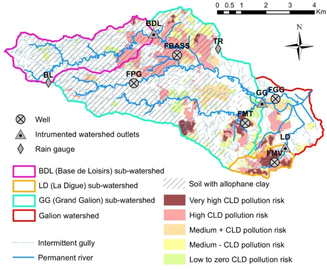
125
Figure 1: Map of the Galion watershed, positions of the 3 sub-watersheds, wells, rain gauges, risk of CLD pollution
126
risk. Pollution risks following the method described in Desprats et al. (2004) and applied by Della Rossa et al.
127
(2017).
128
We monitored the two sub-watersheds BDL (Base de Loisirs - 8.5 km2) and LD (La Digue – 1.9 km2)
129
in addition to the whole GG (Grand Galion) sub-watershed that covers 35.9 km2 (Figure 1). The
130
monitoring of the GG sub-watershed aims at representing the functioning of the whole Galion watershed 131
with widely integrated flow from upstream to downstream. The BDL sub-watershed corresponds to the 132
upstream watershed and its monitoring aims at representing the functioning of the upstream zone. The 133
LD watershed is a small sub-watershed located on extremely polluted soils and its confluence with the 134
Galion River is located downstream the GG outlet. The monitoring of LD aims at representing the 135
functioning of small tributaries. LD has no direct hydrological connection with BDL or GG. 136
2.2 Spatial variability of pollution
137
The 3 monitored sub-watershed (GG, BDL and LD) have different characteristics in terms of risk of 138
pollution (section 2.4.2). Two sub-watersheds have a majority of surface with low risk of pollution, with 139
BDL being the less polluted: 86% with no risk, followed by GG (75%). LD with 29% of low risks area 140
has a majority of its area polluted (Erreur ! Source du renvoi introuvable.). Figure 1 shows that on 141
GG, the polluted areas are mainly located in the intermediate area of the sub-watershed. They are located 142
downstream on BDL and all over the watershed on the small LD sub-watershed because of its very large 143
rate of polluted area. 144
6 Very high risk
1970+1980+1992 High risk (1970or1980)+1992 Medium 1992 Medium 1970 No historical banana BDL 0.5% 11.3% 0.9% 1.1% 86.2% GG 2.2% 14.6% 4.9% 3.4% 74.9% LD 29.7% 27.6% 3.5% 10.5% 28.7%
Table 1 : Percentage of risk of contamination for each watershed (percentage of total area)
145
2.3 Hydrological monitoring and water sampling
146
2.3.1 Rainfall, hydrological and hydrogeological monitoring 147
Daily rainfall for station « Bois Lézard » (BL) and « Trinité Réservoir » (TR) were acquired from Météo 148
France. « Bois Lézard » is located upstream and « Trinité Réservoir » midstream (see Figure 1 for 149
locations). This combination of stations provided an overview of the rainfall gradient from up to 150
downstream. 151
Discharges at the watershed outlets of BDL and LD were measured at a 3 minutes time step using a 152
MS5 sensor (HYDROLAB®) and recorded on DuoSens stations (OTT®). We gauged BDL and LD using
153
current meter and Salinomadd (MADD®). We used the Manning-Strickler relationship based on
154
measurement of sections of the stream to estimate discharge for high water levels. 155
The direction of the environment, management and housing (DEAL) from Martinique performed the 156
GG watershed gauging and hydrological monitoring. Data are accessible through the HYDRO 157
EauFrance website (http://www.hydro.eaufrance.fr/). 158
Groundwater level was recorded in 5 wells (see Figure 1 for location), equipped with automatic 159
piezometric level recorders (OTT®): Malgré Tout (FMT) – depth = 45 m, Mont-Vert (FMV) – 15 m,
160
Bassignac (FBASS) – 50 m, Grand Galion (FGG) – 50 m and Petit Galion (FPG) – 43 m. 161
2.3.2 Water sampling in rivers and wells 162
We sampled water in rivers using two different methods. A first campaign was performed in 2013 by 163
sampling all river confluences within 5 days with punctual (one off) sampling. For more detail, the 164
protocol is described in Della Rossa et al. (2017). 165
The second campaign started in February 2016. We sampled water at the 3 sub-watershed outlets (BDL, 166
LD and GG) with a time dependent sampling protocol. To that purpose, each pollution measurement 167
station was equipped with an automatic sampler: ISCO 6712 (ISCO Incorporation®) sampler on BDL;
168
Sigma SD900 (Sigma®) sampler on GG and LD. Throughout each week, that lasted from Monday to the
169
next Monday unless exception, the sampling frequency of each sampler was set to sample twice 100 mL 170
every 1h15. One sample was stored in a plastic container while the other in a glass container. Both 171
containers were collected once a week meaning that each week the composite sample in each bottle 172
integrated on average 135 samples. At the end of each week, we collected the two containers containing 173
the composite samples and filled the bottles provided by the laboratory (3 glass bottles: 2 x 1 L +100 174
mL and 2 plastic bottles : 2 x 150 mL totaling 2.4 L) with the composite samples stored in the plastic 175
and glass containers. Samples were collected every weeks from 01/02/2016 to 01/02/2018 and sent in 176
ice coolers. 177
From October 2016 to March 2017, GG station was destroyed by a large storm (Matthew). During that 178
period, we performed punctual sampling each week. 179
During our sampling Campaign, French Water Office ODE also sampled water monthly at the GG 180
outlet. Punctual sampling was performed once a month and analyzed by LDA26 for pesticide 181
concentration. 182
For groundwater, sampling was based on standard NF EN ISO 5667-3, and the FD T 90-523-3 and FD 183
X31-615 guidelines. Before sampling in wells, at least three purge volumes were pumped with a 184
7 submersible pump until stabilization of the chemical groundwater parameters. Samples were stored at 185
5°C and shipped in ice coolers before expedition for analysis. 186
2.3.3 Chlordecone analysis 187
We send the aliquots to laboratory for pesticide analysis. The selected LDA26 laboratory has been 188
accredited by Cofrac, the French Accreditation Committee for pesticide analyzes providing guarantees 189
for their technical skills and reliability as well as good management practices. LDA26 complies with 190
ISO 17025 standards for testing and calibration. 191
Laboratory performed liquid/liquid extractions on samples. One liter of water sample was submitted to 192
3 extractions by using 50 mL of a mix of dichloromethane (80%) and ethyl acetate (20%). One cycle 193
was performed at pH 7 and two cycles at pH 2. Extract was concentrated to 1mL in ethyl acetate. The 194
extract was then split into twice 500 µL. 500 µL were use for GC MS and 500 µL for HPLC MS MS. 195
The HPLCC MS-MS was done on two transitions: 506.7/424.5 and 506.7/426.5 with a Sciex API 4000 196
QTRAP. Internal standards used as tracers were hexabromobenzene, tributylphosphate (added at 197
extraction step), 2.4D3, Atrazine D5 (added at injection step) in multiple residual analysis. 198
The validation was done according to NFT 90210 standards. The limit of quantification was determined 199
using six times two repetitions, the reproducibility using at least eight additions of CLD at LOQ at 200
different dates. The trueness, recovery were estimated by using six times two additions of CLD at 3 201
concentrations. Uncertainty was estimated using six times two additions of CLD. 202
A GC quality control is performed every 20 samples at LOQ. Laboratory performed an internal 203
calibration on 5 points before each analysis sequence. CLD addition on matrix and participation to inter 204
laboratory comparison were also performed to control the quality of results. 205
CLD concentrations are given by the laboratory with a ±35% error interval, a limit of quantification 206
(LOQ) of 0.01 µg.L-1, a limit of detection (LOD) of 0.0033 µg.L-1. The extraction efficiency is 89%.
207
2.4 Agricultural practices and risks of soil pollution
208
2.4.1 Actual agricultural practices 209
Surveys on farms located on the watersheds were performed between November 2016 and January 2016. 210
During surveys, decision rules for practices application and plantation dates were inquired. We analyzed 211
the evolution of fallow and crop plantations at the watershed scale using the field geographical register 212
(RPG) from 2016 and 2017 (Direction of Agriculture And Forest of Martinique - DAAF 972). These 213
georeferenced data describe agricultural land uses in 2016 and 2017 as declared by farmers. 214
2.4.2 Mapping the risk of soil pollution 215
The risk of soil pollution by CLD was estimated following the method described in Desprats et al. (2004) 216
and applied by Della Rossa et al. (2017) on the Galion watershed. The method rely on a retrospective 217
analysis of banana land use during the period of CLD application in Martinique (1972–1993). Soil 218
pollution risk was classified according following rule: i) Very high risk for banana plantations present 219
in 1970, 1980 and 1992, ii) High risk for banana plantations present for two out of the three years, iii) 220
Medium + for banana plantations present in 1992 only, iv) Medium - for banana plantations present in 221
1970 only, and v) No historical banana. 222
2.5 Data analysis
223
We compared distributions of CLD concentrations between the two years using the non-parametric 224
Wilcoxon Mann-Whitney test. In order to visualize CLD concentration trends, we applied a Hodrick-225
Prescott filter on the data. This filter was designed to separate long-term trends to short-term variations, 226
suiting our need for pollutants dynamic analysis as previously applied by Sun et al. (2013). The best 227
captures of trend were obtained with lambda parameter: 1600 × 34. The baseflow component of the 228
discharge time series was calculated using the one-parameter recursive digital filter proposed by Lyne 229
8 and Hollick (1979) implemented in the HydRun package (Tang and Carey 2017). The best capture of 230
baseflow component of the discharge time series were acquired with parameter value of 0.8. 231
2.6 Transfers estimation
232
Chlordecone mass transferred at the outlet of each instrumented watersheds was computed for each day 233
using the formula. 234
𝑄𝑐𝑙𝑑 = 𝑊𝑒𝑒𝑘𝑙𝑦𝐴𝑉𝐺𝐶𝐿𝐷 ∗ 𝑑𝑎𝑖𝑙𝑦𝐷𝑖𝑠𝑐ℎ𝑎𝑟𝑔𝑒 ∗
3600 ×24
1000 (1)
235
With 𝑄𝑐𝑙𝑑 the daily mass of CLD transferred at outlet (g), 𝑊𝑒𝑒𝑘𝑙𝑦𝐴𝑉𝐺𝐶𝐿𝐷, the weekly average CLD 236
concentration in water samples (µg.L-1) and 𝑑𝑎𝑖𝑙𝑦𝐷𝑖𝑠𝑐ℎ𝑎𝑟𝑔𝑒 the average daily discharge at sampling
237
point (m3.s-1). The other term is a unit conversion factor.
238
We calculated the daily mass of CLD transferred at outlet per unit of polluted area (classified in low, 239
medium-, medium+, high or very high risks) by dividing 𝑄𝑐𝑙𝑑 by the polluted surface of each sub-240
watershed estimated with the methodology described in 2.4.2. 241
3 Results
242
3.1 Evolutions of CLD concentration in rivers
243
3.1.1 Infra-annual evolution 244
Rainfall, discharge and CLD concentrations recorded on the 3 monitoring stations are presented in 245
Figure 2. The proximity of rainfall and flood peaks for the 3 stations on a daily basis, illustrated that the 246
watershed quickly reacted to rainfall events at the sub-watershed as well as the watershed scales. 247
Reaction time of each watershed or sub-watershed was less than one day. 248
9
Figure 2 : Hydrology and chlordecone dynamics on the 3 sampling sites of the watershed. Red dots: ODE data.
250
Grey lines on CLD concentration graphics: Hodrick-Prescot filter and ±35% error interval. Grey dashed lines on
251
discharge graphics: baseflow. Orange vertical line: Matthew storm.
252
Figure 2d and 2f shows that the trend of the CLD concentrations were correctly assessed by the Hodrick-253
Prescott filter at BDL and LD stations because most measurements fell within the ±35% interval around 254
the filtered values which correspond to the laboratory analytical uncertainty on CLD concentration 255
measurements. Deviations from the trend may also results from shorter wavelength processes, such as 256
flooding, sampling uncertainty, organic matter or sediments in samples. The dynamics highlighted by 257
the filter showed patterns with period of increasing and decreasing concentrations. The up and down 258
trends highlighted by the filter were within the same periods on BDL and LD stations. According to this 259
result, it is likely that the dynamics we observed had a common causality. We observed that short-term 260
increase of baseflow is associated with CLD concentration decrease on all stations, while short-term 261
baseflow decrease are associated with CLD increase (see between 02/2016 and 09/2016 - Figure 2). 262
During that period, CLD concentrations decrease on all station between 02/2016 and 04/2016, then it 263
increased between 04/2016 and 05/2016, and decreased again between 05/2016 and 07/2016. This 264
behavior corresponds to the hydrological functioning of the watershed and subwatersheds subjected to 265
small hydrological variations where the baseflow in not subjected to changes in regimes that last more 266
than few months. A finer analysis on the trends showed that an uptrend started few time after the 267
“Matthew” storm (29/09/2016) when baseflow decreased and ended in March 2017. The trends were 268
more difficult to assess on the GG station (Figure 2b) due to the lack of integrated data between 10/2016 269
and 03/2017 after debris transported in water few time after the Matthew storm destroyed our station. 270
In fact, punctual sampling at that time showed high values: from 12/2016 to 04/2017 in particular, 12 271
punctual samples out of 15 had CLD concentrations higher than 1.1 µg.L-1 while the average
272
concentration from 02/2016 to 02/2018 was 0.75 µg.L-1. The ODE follow up also suggested high CLD
273
concentrations during that period. Starting from June, ODE data followed a bell shaped dynamic while 274
our integrated sampling did not. In fact, concentrations measured by ODE decreased while the values 275
of our integrated measurements increased (see 10/2017 in Figure 2b). Punctual sampling results diverged 276
from the ones we obtained with integrated sampling indicating that CLD trends should not be easily 277
deduced from punctual sampling at the infra-annual temporal scale. 278
To summarize, we identified general trends in the dynamics of CLD according to our integrated 279
sampling. It showed a good consistency between stations LD and BDL that have no direct hydrological 280
connection. However, we also identified that punctual weekly samples led to record high variations of 281
concentrations. It prevents from assessing trends of CLD concentration on punctual sampling and justify 282
assessing CLD concentrations on a weekly basis. 283
3.1.2 Inter-annual evolution 284
The inter-annual dynamics on LD (Figure 2f), highlighted an increase of CLD concentration in early 285
2017. Then, until late 2017, these concentrations remained higher than in 2016 (Table 2). Comparing 286
average concentration between 2016 and 2017, we observed i) a slight increase of CLD average 287
concentration on GG watershed (+15%), ii) average concentrations on BDL that remained stable over 288
the two years, and iii) that CLD average concentration almost doubled (+82%) between 2016 and 2017 289
on the LD watershed. However, average concentrations did not reflect distribution of pollution between 290
the two years The distributions of concentrations recorded in 2016 and 2017 were significantly different 291
for all sub-watersheds, being highly significant for GG and LD sub-watersheds (p-value<0.001), but in 292
a lower extent for BDL sub-watershed (p-value<0.05). This result shows that, on BDL, similar average 293
concentration (0.46 µg.L-1) resulted from different river behavior in 2016 and in 2017 (significantly
294
different distributions). Indeed, the trend analysis of BDL station showed that 2016 was characterized 295
by a stable CLD concentration surrounding 0.46 µg.L-1, while concentrations recorded during 2017 were
296
more variable with a CLD peak (>2 µg.L-1 - 03/2017) followed by an overall decrease of the
297
concentration (<0.46 µg.L-1) before returning to the initial value in 10/2017 (0.46 µg.L-1) (Figure 2d).
10 Since we noticed in section 3.1.1 that LD and BDL have CLD trends showing similarities, the high 299
increase in mean CLD concentration in 2017 for LD stemmed, on the one hand, from two CLD peaks 300
instead of one for BDL and, on the other hand, from higher CLD contents after the first peak relative to 301
Matthew storm. This may be explained by the fact that the stabilized increase of CLD concentration in 302
LD in 2017 is related to a higher baseflow level than in 2016 (Figure 2e and f). The fact that this small 303
watershed is mainly drained by subsurface flows make it more responsive to modifications of land uses 304
for instance. Such relationship with baseflow was not observed on BDL or GG. However, it might be 305
that the increase of CLD concentration we observed on GG between 10/2017 and 01/2018 has the same 306
origin but delayed in time because it is 19 times larger than LD. 307 Sampling site CLD Mean (2016) (µg.L-1) CLD Mean (2017) (µg.L-1) GG 0.70 0.81 BDL 0.46 0.46 LD 5.54 10.08
Table 2 : Average chlordecone concentration on the 3 sampling points for the 3 sampling campaigns (2013, 2016
308
and 2017).
309
Monitoring CLD concentrations on the 3 stations showed that CLD is a relatively stable and chronic 310
pollution in rivers. We showed that the CLD dynamics observed in river has two components: a trend 311
of inter-annual evolution that may be driven by baseflow as well as infra-annual variations surrounding 312
that trended evolution whose intensities vary according to stations and may be driven by specific event 313
like storms in the present case. 314
3.1.3 Mass transfers 315
The average daily CLD mass transferred at the outlet of each sub-watershed, as well as the average daily 316
CLD mass transferred per unit of area polluted by CLD are presented in Table 3. According to Erreur ! 317
Source du renvoi introuvable., we deduced potentially polluted area on the 3 sub-watersheds: 116 ha 318
for BDL, 901 ha for GG and 136 ha for LD, meaning that the area between GG and BDL holds 785 319
potentially polluted hectares. The highest values of daily average CLD transferred at outlet were 320
recorded on GG, while lowest values were recorded on BDL (Table 3). 321 2016 2017 Daily average (g.day-1) Daily average per unit of polluted area (g.day-1.ha-1) Specific discharge (m3.s-1.km-2) Daily average (g.day-1) Daily average per unit of polluted area (g.day-1.ha-1) Specific discharge (m3.s-1.km-2) GG 91±171 0.10 0.047 137±303 0.15 0.065 LD 52±169 0.38 0.052 68±124 0.5 0.042 BDL 49±24 0.42 0.147 51±53 0.44 0.144 GG-BDL 49±159 0.06 0.018 97±266 0.12 0.027
Table 3 : Chlordecone mass transferred by each watershed monitored
322
Table 3 shows that sub-watersheds with larger polluted area (GG and GG-BDL) are not necessarily the 323
one that transfers the most CLD toward our monitored outlet. BDL and LD having transfers rates by 324
polluted area 4 times higher that GG or GG-BDL (Table 3). It means that in terms of mass, the area 325
between BDL and GG, in spite of large potentially polluted area had a lower transfer’s rate to outlet. 326
The upstream zone (represented by BDL) is humid with large rainfall and characterized by a larger 327
specific discharge than the other sub-watersheds (Table 3). Large water volumes at relatively low CLD 328
concentrations generated stabilized transfers at outlet as shown by the lower standard deviation than on 329
GG or LD (Table 3). This also means that GG and LD are more subject to large variations of daily CLD 330
mass transferred. The small specific discharge of GG-BDL also indicate that the area between GG and 331
BDL has a small contribution to the discharge. Our results also shows that LD, in spite of its small size 332
11 (191 ha) and low discharge compared to GG or BDL, transfers unneglectable mass of CLD because of 333
very high water CLD concentrations. 334
Daily mass transferred by GG gave annual values from 33 kg.y-1 to 50 kg.y-1 of CLD transferred to the
335
Galion Bay. For LD watershed, annual value transferred to the Galion bay ranged from 19 kg.y-1 to 25
336
kg.y-1. This means that the total yearly contribution of that two outlets to the Galion bay may be
337
estimated from 50 kgCLD.y-1 to 75 kgCLD.y-1. Using a simple assumption of constant transfer rate, and
338
without considering years of applications, we estimated total transfers to the bay from 1993 to 2018 to 339
be between 2500 kg and 3750 kg. This might be even more because we did not took into account 340
transfers from 1970 to 1993. These amounts represent between 2.4 and 3.6 kgCLD per ha of polluted 341
area. This is low compared to the amount of CLD applied ≈3 kg.ha-1 at each application (Cabidoche et
342
al. 2009; Levillain et al. 2012) during more than 20 years. Calculations of CLD stocks in soils according 343
to Levillain et al. (2012) gave values of few kg of CLD stocked in soils in the 0-60 cm depth. This 344
suggests that, it is very likely that large amounts of CLD already transferred to other environmental 345
compartments, meaning that substantial amount of CLD could be in the marine environment and in 346
aquifers. Because CLD was applied around banana stems and banana fields were mainly cropped on 347
bare soils with stemflow at that period (Charlier et al. 2009) that conjointly favors surfaces transfers. It 348
is likely that the larger fraction of CLD that lacks in our CLD balance went mainly to the marine 349
environment during storms towards fast surface transfer processes such as runoff or subsurface flows, 350
both concentrated in surface drains that were a very common on banana field at that time. 351
We showed that small watershed can nowadays have significant chlordecone transfers contributions to 352
the ocean. In spite of the potentially large amounts of CLD that transferred in the past, we suggest that 353
such areas with fast hydrological response should be managed with care and prioritized for pesticides 354
reduction strategies as well as decontamination. We expect that the results of mitigation measures could 355
be observable in the river in a couple of years for these areas. 356
3.2 Evolutions of CLD in groundwaters
357
Piezometric levels on the 5 wells located on the watershed and CLD concentrations recorded in 4 of 358
these aquifers are presented in Figure 3: FPG (Fig.3b), FMT (Fig.3c), FBASS (Fig3d), FMV (Fig3e). 359
FBASS an FMT are deep aquifers while FGG, FPG, and FMW have piezometric levels around few 360
meters. CLD concentrations in groundwaters located in contaminated areas were 10 to 50-fold higher 361
than concentrations measured in rivers (Figure 2 and 3). No chlordecone was found in FPG waters that 362
is consistent with its location upstream the polluted areas (Figure 1). Based on the punctual data set, we 363
can say that the CLD concentrations in aquifers varied along the year, but we could not define a clear 364
relationship between CLD concentrations and piezometric levels due to the scarcity of sampling. All 365
aquifers sampled on the 03-11-2016, at the beginning of the high water level period, had particularly 366
high CLD concentrations. Then, CLD concentrations decreased in the following samples (Figure 367
3b,d,e), but remained always in a high range of values. Besides, each aquifer had its own piezometric 368
dynamic as shown in Figure 3. For instance, FMT had more inertial dynamic than FBASS or FMV, and 369
even more than FGG or FPG. According to Charlier et al. (2015), the dynamic between recharge and 370
discharge to rivers can be very long for deep aquifers with residence times from 4 years (FMV), 6 to 8 371
years (FMT) to more than 20 years (FBASS). 372
12 373
Figure 3 : Piezometric levels and CLD concentrations in aquifers of the Galion watershed. Black dots: chlordecone
374
concentrations. Grey lines: analytical uncertainty on chlordecone concentrations.
375
3.3 Evolutions of agricultural practices
376
CLD polluted soil of the watershed are still mainly cropped with banana tree. This is because CLD is 377
not quantified in banana fruit even when cropped on highly polluted soils (Clostre et al. 2017). CLD 378
being stored into soil, several grower practices might affect CLD transfers. According to our banana 379
grower survey, we could draw a general cropping system practiced by banana growers. Banana cropping 380
system usually last around 7 years. During those 7 years, 5 or 6 years are indeed cropped with banana 381
and the remaining 1 or 2 years consist in a fallow period. The fallow period allows for the soil to rest 382
and eliminates diseases that developed in soil (nematodes and weevils) during the repeated banana 383
cropping cycles. The fallow is established using herbicide injected into banana trees to kill them. Then, 384
soil is tilled (Figure 4b). A fallow cover crop may either be planted, for instance with C. spectabilis or 385
B. decumbens, or results from spontaneous species (such as C. ruditosperma). Depending on farms, at 386
the end of the fallow period, either soil is tilled again before plantation, or banana tree are planted in a 387
mulch of plants killed with herbicide. On the farms of the Galion watershed, tillage is usually carried on 388
before or during the fallow period. 389
Figure 4a shows the field of one farmer of the LD watershed right after the Matthew storm. This farmer 390
cut all developed banana tree in its farm (25 ha out of the 79 ha of cropped area by all farmers on the 391
watershed) because most developed trees were laid down by the storm. 392
13 393
Figure 4 : a) Cycloned field just after the Matthew storm on the La Digue (LD) sub-watershed (C. Mottes 394
Oct-2016). b) Fallow (grass with dead banana tree on the left) been tilled with excavator (bare soil) on 395
the La Digue (LD) sub-watershed (C. Mottes Apr-2017). 396
Figure 5 shows fallows surface evolution between 2016 and 2017. We can see that 2017 was 397
characterized by large increase of fallow area on the watershed that almost doubled: in 2016 fallow 398
covered 79 ha whereas it covered 139 ha in 2017. This means that larger area than usual were tilled on 399
the watershed between 2016 and 2017. This practice of large fallow integration after a cyclone or a 400
violent tropical storm is a common practice among banana growers in the FWI resulting in large-scale 401
modification of agricultural practices. 402
403
Figure 5: Evolution of fallow and banana between 2016 and 2017 (data from RPG 2016 and 2017 DAAF).
404
4 Discussion
405
4.1 CLD evolutions in rivers and aquifers
406
Our results showed that river and aquifer pollutions by CLD was roughly stable and chronic. Several 407
authors have reported this (Crabit et al. 2016; Mottes et al. 2015; Mottes et al. 2017). However, CLD 408
concentrations in rivers vary according to sites. On the small LD subwatershed, we showed that CLD 409
interannual variability observed in river may be driven by baseflow. In the case of watersheds draining 410
14 the highest reliefs of volcanic islands, Crabit et al. (2016) found correlation between CLD concentration 411
and discharge because the main process of CLD evolution was the dilution of water drained from lateral 412
cultivated areas by high amounts of unpolluted waters from the forested areas upstream. In the case of 413
watersheds draining mostly cultivated zones, Mottes et al. (2016) did not find such relationship on the 414
Ravine watershed, highlighting complex conditions of CLD transfers. At the watershed scale, Della 415
Rossa et al. (2017) showed that the spatial variability of CLD concentration in water during low flow 416
periods was explained by the potential pollution of the fields located on the watershed of the sampled 417
points. At the regional scale, comparing numerous watersheds in Martinique Island, Cattan et al. (2019) 418
showed that the spatial variability of CLD concentration may be explained by a combination of the 419
location of banana cropping areas, soil and geological factors; these conditions defining a high diversity 420
of situations in terms of the mid- to long-term duration of pollution. 421
Unlike previous studies, our results highlights that, at a weekly time step, CLD concentrations in rivers 422
showed annual evolution trends (Figure 2). Aquifers located in polluted area (Figure 1) showed higher 423
CLD concentrations during recharge (Figure 3) then followed by CLD uptrends in rivers (Figure 2). 424
Figure 2 and Figure 3 analyzed conjointly showed that the uptrends we observed in rivers followed the 425
generalized CLD peak in aquifer observed in 11/2016. Here, we are in the opinion that CLD 426
concentration increased in aquifers and rivers as the consequence of, either translatory flow (Lischeid et 427
al. 2002), or recent leaching of water highly concentrated with CLD. This suggests that surrounding that 428
time, factors generated an increase of CLD leaching to aquifers and subsurface flows. 429
430
4.2 Factors explaining increased CLD leaching
431
Increased CLD leaching from soils, that is still a large reservoir of CLD (Lesueur-Jannoyer et al. 2012), 432
to aquifers and subsurface flows is likely to have generated the increases of CLD concentrations in 433
aquifers and rivers we observed. Several factors that increase the availability of CLD into soil to water 434
flows can explain an increase of CLD leaching. 435
4.2.1 Effect of hydroclimatic conditions 436
Our results showed higher CLD concentrations on all wells situated in polluted area on the watershed at 437
a specific date: 03-11-2016 but we could not conclude on a relationship with piezometric levels. This 438
pattern is coherent with previous works carried out in similar hydrogeological context in Martinique 439
Island by Arnaud et al. (2016). Based on a higher resolution of sampling (monthly), these authors 440
showed that the intensity of piezometric fluctuations was not correlated with the amplitude of variations 441
in CLD concentration, but that the CLD higher concentrations were often observed during periods of 442
rising groundwater levels. Our results suggest that period of soil drying may increase the availability of 443
CLD to water flow during the first leaching events. This is in accordance with the observations of 444
Arnaud et al. (2016), showing that the main CLD peak in groundwaters from the last decade occurred 445
during the first major recharge event after a several year period of deficient recharge that resulted in a 446
very low water table. This was true for 8 wells located all over the contaminated zones of the Martinique 447
Island, meaning that such regional pattern is likely controlled by hydroclimatic conditions. Following 448
this explanation, we expect that the main CLD higher concentrations observed in rivers of the Galion 449
watershed after the storm of October 2016 is related to the higher groundwater concentrations observed 450
at that time. 451
4.2.2 Effects of cropping practices 452
CLD applications were forbidden after 1993, so that theoretically no applications occurred from that 453
date. As a result, the only agricultural practices that could have increased CLD leaching are the one that 454
modified environmental characteristics that affect pesticide transfers (Mottes et al. 2014). Here, 455
modifications of the soil organic matter content, allophane clay content, or both potentially decreased 456
CLD retention by soil (Woignier et al. 2016; Woignier et al. 2012a; Woignier et al. 2012b; Woignier et 457
al. 2013). It has been shown that the peculiar hierarchical (fractal) microstructure of allophane clay traps 458
CLD (Woignier et al. 2012a; Woignier et al. 2013). It is known that tillage activate soil organic matter 459
15 decomposition (Haddaway et al. 2017) and expose soil to direct sunlight, hence, to strong drying at its 460
surface resulting in destruction of allophane (Quantin 1972) and allophane microstructure. During 461
drying, the fractal microstructure progressively disappears (Woignier et al. 2008). As a result, tillage 462
would act on both degradation of soil organic matter and allophanes trapping properties in andosols. On 463
top of that, tillage destroy the soil structure. The destruction of the soil structure imply a modification 464
of the water paths into soil (Alletto et al. 2010). Indeed, structured soils present preferential infiltration 465
flow that may be washed from extractible CLD after several time. Destroying those paths induce water 466
to access more porosity in soil and thus extract more CLD from soil. This may explain the difference of 467
one order of magnitude found in CLD soil organic carbon coefficients (Koc) between modelling field 468
studies (Cabidoche et al. 2009; Mottes et al. 2015) and laboratory data (Baran and Arnaud 2013; 469
Fernandez-Bayo et al. 2013a). In the last, soils are totally destroyed (Oecd 2000) while in the first one 470
structured soils are considered. Finally, tillage induces modifications of soil organic matter and clay 471
characteristics are modified as well as the soil structure. All these evolutions favor the leaching of CLD. 472
The modification of water path in soil could results from tillage but mays also results from modifications 473
of soil covers. According to Lewis et al. (2016) and to Mottes et al. (2014) practices that modify ground 474
cover may modify pesticide leaching. This is particularly true for vegetative ground cover such as 475
banana tree. According to several authors, we know that banana trees concentrate rainfall along their 476
stem by a process called stemflow (Cattan et al. 2007; Charlier et al. 2009; Sansoulet et al. 2008). This 477
means that, in a cropped banana field, water will preferentially infiltrate right under banana tree (Cattan 478
et al. 2007; Sansoulet et al. 2008) generating preferential flow paths under banana tree. As for structured 479
soil, we can expect that such preferential water path are “washed” from CLD after several time of semi-480
perennial banana cropping. Stemflow was also shown to increase runoff (Charlier et al. 2009), meaning 481
that this process also acts on reducing the overall leaching on banana fields. Consequently, stemflow 482
increases erosion of particulate CLD transfers as well as other surface pollutant transfers. To conclude, 483
it means that any modification that reduce stemflow is likely to increase leaching on the field. 484
Our results showed that between 2016 and 2017 the surface of tilled polluted fields increased (Figure 5) 485
on all monitored sub-watershed. Figure 1 shows that most soils of the watersheds contain allophane 486
clay, meaning that either tillage, dry period or both could have resulted in CLD uptrend. This means that 487
it increased the access of CLD to leaching water in 2017. Such processes could have generated 488
increasing CLD concentration in subsurface flows thus generating uptrends in river CLD concentrations 489
we observed on LD and BDL. 490
4.3 Integration of processes at the watershed scale
491
Our results showed that the different aquifers have contrasted piezometric inertia (Figure 3). In the 492
Galion watershed, Charlier et al. (2015) showed variable mean residence times varying from 4 years 493
(FMV), 6 to 8 years (FMT) to more than 20 years (FBASS). They also reported smaller residence times 494
of one year for sources or during high water levels. Because, rivers in FWI are mainly governed by 495
underground flows (Charlier et al. 2008; Crabit et al. 2016; Mottes et al. 2015), this means that, at the 496
watershed scale the river is likely to be fed by different aquifer’s units having different inertia. The 497
combination of residence times and the multiplicity of aquifers contribute to the stability of CLD 498
concentration at the weekly time step. According to our results along with the ones of Charlier et al. 499
2015, there is every likelihood that only underground major contributors changing conjointly may 500
modify the trend of CLD concentration in rivers. The increased CLD concentration at LD confirms this. 501
LD watershed is mainly governed by subsurface flow and the monitored aquifer (FMV) has a short mean 502
residence time of 4 years, allowing it to be sensitive, among others, to strong cyclonic events. Our results 503
showed that the mid-term CLD concentration increase in 2017 is related to the increase of the baseflow 504
on this river (Figure 2e). According to our results, we are in the opinion that increasing CLD 505
concentrations rely on the activation of new water paths on polluted areas on the sub-watershed. 506
507
Our results showed that in rivers, CLD concentration in punctual and integrated sampling diverged 508
(Figure 2b). This behavior was unexpected, because we would expect to see both monitoring programs 509
16 showing the same dynamics for a chronic pollution such as CLD. One explanations could be that CLD 510
concentrations shows large variations with time at the event scale as it was shown for CLD (Mottes et 511
al. 2016) and for other pesticides (Liger et al. 2012). The variability of CLD concentrations we obtained 512
when we performed weekly punctual sampling instead of integrated sampling (between Oct 2016 and 513
April 2017) supports that hypothesis because CLD concentration variation are very high at that period. 514
This could mean that integrated sampling integrates the contributions of the different zones of the 515
watersheds taking into account the delayed transfers’ times according to positioning on the watershed. 516
The CLD concentration trend we measured corresponds to the evolution of average concentrations that 517
integrates such variability. A variable transfers time according to positioning on the watershed was 518
suggested by Mottes et al. (2015) who included a delay in modelling CLD transfers into river according 519
to the distance of contributing areas. On large watershed, this short-term effect might be buffered at the 520
weekly time step or induce larger dynamics on CLD transfers. On that point, our results showed that the 521
spatial organization of polluted fields differed in the 3 sub-watersheds, with LD being polluted on almost 522
all its area, BDL downstream and GG mid-stream. It could be that the spatial organization of polluted 523
area affected the CLD dynamics observed at the watershed scale (Figure 2): BDL showed uptrend 524
followed by downtrend that could correspond to downstream contributions followed by upstream 525
contributions. As a result, the variation of CLD concentration of punctual and integrated sampling might 526
results from the contributions of the different transfer times of surface and subsurface flow generating a 527
dynamics at the short to mid-time scale depending on the size of the watershed. 528
CLD short terms variation could also come from the fact that sediments interacts with CLD in the 529
dissolved phase, especially in the sampling containers of our sampling stations. With automatic 530
integrated samplers, erosion events are sampled along the week with water. As a result, sediments enters 531
into the sampling container. They could increase CLD concentration in the sample because of CLD 532
bound to sediments. According to ODE data, sediments analyzed at the GG station between 2008 and 533
2015 revealed CLD concentration varying between <10 µg.kg-1 and 30 µg.kg-1. These values are low
534
compared to soil CLD concentrations (0.1 – 5 mg.kg-1), but could be sufficient to modify CLD
535
concentrations in sampling containers according to the concentration value measured (Table 2) (Katagi 536
2006). Finally, higher variability of punctual sampling may be related to the difficulty to follow the 537
same protocol at each sampling date. Notably sampling site may differ according to the possibilities of 538
access to the river. 539
Our results suggest either that there are variability of CLD concentrations at the instant time scale or a 540
strong interaction between dissolved and particulate phases. This means that the average concentration 541
we obtain in weekly samples results from CLD trends, variations of CLD concentrations all over the 542
week and from sediment dynamics in the river. 543
4.4 How to manage CLD pollution ?
544
Our results showed that causes and processes that modify CLD concentration in water, are interrelated, 545
making it difficult to isolate single effects. A complexity exists at the watershed scale where different 546
organization levels and processes interact. Agricultural practices triggered according to climatic 547
windows stand for an example of such interaction. Banana is still mainly cropped on polluted soils 548
because it is not sensitive to soil pollution by CLD. Banana farming practices follow decision rules 549
based on climate (cyclonic season, dry season), market.... Banana plantations increase in July to reach 550
good price marked at the first harvest. Fallow, are largely practiced post-cyclonic after banana trees are 551
laid down by high speed winds. Tillage is easier and recommended at medium humidity conditions 552
corresponding to conditions of the beginning or of the end of the dry season. This means that monitoring 553
of CLD in river will always show systemic response to event such as storm of cyclones. After them, 554
large recharge occurs, stemflow disappear, tillage and fallow are practiced during dryer periods, all these 555
potential causes of CLD increase have a similar triggering event, which is the storm. In a counterpart, it 556
means that we can acts on several leeways at the watershed scale. In a mid-term objective, we 557
recommend to integrate knowledge on pesticides transfers at different scale into modelling tools such 558
17 as WATPPASS (Mottes et al. 2015) and to adapt their formalism to help farmers along with extension 559
workers and decision makers to test and assess the effect of different scenarios on CLD transfers. Test 560
the collective response of farmers at the watershed scale to specific climatic events such as storm that 561
actually induce practice response with deleterious effects on CLD concentrations. 562
Our analysis showed that processes at different scale interact. Because, we cannot act on the aquifers-563
river relationship, we recommend focusing on limiting transfers from polluted fields. To that point, we 564
showed that hot spots, such as LD watershed are heavy polluted by CLD resulting in large CLD 565
concentrations in water. Such high concentration results in large amount transferred at outlet and 566
reaching the marine environment. At the watershed scale, we recommend to focus management of 567
transfers, on that kind of area for 3 major reasons. First, in spite of their small surface, they are large 568
contributor to pollution transfers. Second, according to our results, such small watershed react quicky 569
to practices and hydroclimatic conditions so that monitoring will be able to assess the positive impact 570
of practices change on water quality. Third, they are managed by less farmers, making it easier to 571
consistently manage all fields from the zone. 572
Decontamination of soils remains the final objective (Chaussonnerie et al. 2016; Mouvet et al. 2017). In 573
the meanwhile, in terms of actions, we showed that tillage that active different processes favoring CLD 574
transfers should be avoided as much as possible on polluted soils, or at least positioned on specific area 575
where required such as plantation lines. To avoid pollution peaks, we recommend to avoid long drying 576
of soils, in particular soils with allophanic clays. Maintaining a ground cover and a minimal controlled 577
irrigation to maintain minimal hydratation could help reduce CLD peak at the end of the dry season. 578
Sequestration method using organic matter could be applied (Clostre et al. 2014). Using farm available 579
organic matter, returning large amount of crop residues, the use of grass or covercrop to produce large 580
amount of OM returned to soil, and bringing externals sources of OM from unpolluted fields could help 581
increase OM concentration that stabilize CLD into soils. 582
5 Conclusion
583
We showed that CLD s concentrations vary at different spatial and time scale. The large variability of 584
biophysical and decisional processes as well as their interactions at that scale require a systemic 585
approach for their understanding and management. Such systemic analysis requires a local 586
characterization of the hydrogeological functioning and of the agricultural practices to better understand 587
losses in rivers. In the French West Indies, these involves historical CLD application, soil characteristics 588
and the modifications by agricultural practices, and the reload conditions of aquifers defined by climatic 589
events and the permeability of underground geological formations modulating transfers times. 590
6 References
591
Alletto L, Coquet Y, Benoit P, Heddadj D, Barriuso E (2010) Tillage management effects on pesticide 592
fate in soils. A review Agron Sustain Dev 30:367-400 doi:10.1051/agro/2009018 593
Arnaud L, Charlier J-B, Ducreux L, A.-L. T (2016) Groundwater Quality Assessment. In: Lesueur-594
Jannoyer M, Cattan P, Woignier T, Clostre F (eds) Crisis Management of Chronic Pollution: 595
Contaminated Soil and Human Health. CRC Press, Boca Raton, pp 55-72 596
Baran N, Arnaud L (2013) Mapping of groundwater risks of contamination by pesticides in Martinique, 597
BRGM (in French) 598
Cabidoche YM, Achard R, Cattan P, Clermont-Dauphin C, Massat F, Sansoulet J (2009) Long-term 599
pollution by chlordecone of tropical volcanic soils in the French West Indies: A simple leaching 600
model accounts for current residue Environ Pollut 157:1697-1705 601
doi:10.1016/j.envpol.2008.12.015 602
Cattan P, Cabidoche Y, Lacas J, Voltz M (2006) Effects of tillage and mulching on runoff under banana 603
(Musa spp.) on a tropical Andosol Soil and Tillage Research 86:38-51 604
doi:10.1016/j.still.2005.02.002 605
18 Cattan P, Charlier JB, Clostre F, Letourmy P, Arnaud L, Gresser J, Jannoyer M (2019) A conceptual 606
model of organochlorine fate from a combined analysis of spatial and mid- to long-term trends 607
of surface and ground water contamination in tropical areas (FWI) Hydrol Earth Syst Sci 608
23:691-709 doi:10.5194/hess-23-691-2019 609
Cattan P, Voltz M, Cabidoche YM, Lacas JG, Sansoulet J (2007) Spatial and temporal variations in 610
percolation fluxes in a tropical Andosol influenced by banana cropping patterns J Hydrol 611
335:157-169 doi:16/j.jhydrol.2006.11.009 612
Charlier J-B, Cattan P, Moussa R, Voltz M (2008) Hydrological behaviour and modelling of a volcanic 613
tropical cultivated catchment Hydrol Process 22:4355-4370 doi:10.1002/hyp.7040 614
Charlier J-B, Lachassagne P, Ladouche B, Cattan P, Moussa R, Voltz M (2011) Structure and 615
hydrogeological functioning of an insular tropical humid andesitic volcanic watershed: A multi-616
disciplinary experimental approach J Hydrol 398:155-170 doi:10.1016/j.jhydrol.2010.10.006 617
Charlier JB, Arnaud L, Ducreux L, Ladouche B, Dewandel B (2015) CHLOR-EAU-SOL – Water – 618
Caracterization of water and soil contamination by chlordecone of watersheds in Guadeloupe 619
and Martinique. Final report. BRGM (in French) 620
Charlier JB, Moussa R, Cattan P, Cabidoche YM, Voltz M (2009) Modelling runoff at the plot scale 621
taking into account rainfall partitioning by vegetation: application to stemflow of banana (Musa 622
spp.) plant Hydrol Earth Syst Sci 13:2151-2168 doi:10.5194/hess-13-2151-2009 623
Chaussonnerie S, Saaidi P-L, Ugarte E, Barbance A, Fossey A, Barbe V, Gyapay G, Brüls T, Chevallier 624
M, Couturat L, Fouteau S, Muselet D, Pateau E, Cohen GN, Fonknechten N, Weissenbach J, Le 625
Paslier D (2016) Microbial Degradation of a Recalcitrant Pesticide: Chlordecone Frontiers in 626
Microbiology 7:2025 doi:10.3389/fmicb.2016.02025 627
Clostre F, Cattan P, Gaude JM, Carles C, Letourmy P, Lesueur-Jannoyer M (2015) Comparative fate of 628
an organochlorine, chlordecone, and a related compound, chlordecone-5b-hydro, in soils and 629
plants Sci Total Environ 532:292-300 doi:10.1016/j.scitotenv.2015.06.026 630
Clostre F, Letourmy P, Lesueur-Jannoyer M (2017) Soil thresholds and a decision tool to manage food 631
safety of crops grown in chlordecone polluted soil in the French West Indies Environ Pollut 632
223:357-366 doi:10.1016/j.envpol.2017.01.032 633
Clostre F, Woignier T, Rangon L, Fernandes P, Soler A, Lesueur-Jannoyer M (2014) Field validation 634
of chlordecone soil sequestration by organic matter addition Journal of Soils and Sediments 635
14:23-33 doi:10.1007/s11368-013-0790-3 636
Crabit A, Cattan P, Colin F, Voltz M (2016) Soil and river contamination patterns of chlordecone in a 637
tropical volcanic catchment in the French West Indies (Guadeloupe) Environ Pollut 212:615-638
626 doi:http://dx.doi.org/10.1016/j.envpol.2016.02.055 639
Della Rossa P, Jannoyer M, Mottes C, Plet J, Bazizi A, Arnaud L, Jestin A, Woignier T, Gaude J-M, 640
Cattan P (2017) Linking current river pollution to historical pesticide use: Insights for territorial 641
management? Sci Total Environ 574:1232-1242
642
doi:http://dx.doi.org/10.1016/j.scitotenv.2016.07.065 643
Desprats JF, Comte JP, Charbier C (2004) Mapping of the risk of soil pollution by organochlorine 644
pesticides in Martinique. BRGM (in French) 645
Devault DA, Laplanche C, Pascaline H, Bristeau S, Mouvet C, Macarie H (2016) Natural transformation 646
of chlordecone into 5b-hydrochlordecone in French West Indies soils: statistical evidence for 647
investigating long-term persistence of organic pollutants Environmental Science and Pollution 648
Research 23:81-97 doi:10.1007/s11356-015-4865-0 649
Dorel M, Roger‐Estrade J, Manichon H, Delvaux B (2000) Porosity and soil water properties of 650
Caribbean volcanic ash soils Soil Use Manag 16:133-140 doi:10.1111/j.1475-651
2743.2000.tb00188.x 652
Dromard CR, Guéné M, Bouchon-Navaro Y, Lemoine S, Cordonnier S, Bouchon C (2018) 653
Contamination of marine fauna by chlordecone in Guadeloupe: evidence of a seaward 654
decreasing gradient Environmental Science and Pollution Research 25:14294-14301 655
doi:10.1007/s11356-017-8924-6 656
Fernandez-Bayo JD, Saison C, Geniez C, Voltz M, Vereecken H, Berns AE (2013a) Sorption 657
characteristics of chlordecone and cadusafos in tropical agricultural soils Current Organic 658
Chemistry 17:2976-2984 659