Communications Biophysics

(1)

XII. COMMUNICATIONS BIOPHYSICS

Academic and Research Staff

Prof. L. D. Braida Prof. W. M. Siebert Dr. E. P. Lindholm Prof. S. K. Burns Prof. T. F. Weisstf** D. W. Altmannt Prof. H. S. Colburnt Dr. J. S. Barlowtt R. M. Brownt Prof. L. S. Frishkopf Mr. N. I. Durlach D. J. Callahan Prof. J. L. Goldsteint Dr. R. D. Hall A. H. Cristt Prof. J. J. Guinan, Jr.t Dr. N. Y. S. KiangT W. F. Kelley Prof. R. G. Markj Dr. H. J. Liff L. H. Seifel

Prof. W. T. Peaket S. N. Tandon

Graduate Students

T. Baer B. L. Hicks R. Y-S. Li

J. E. Berliner A. J. M. Houtsma E. C. Moxon

R. Cintron T. W. James V. Nedzelnitsky

P. Demko, Jr. P. B. Jergens W. M. Rabinowitz D. O. Frost D. H. Johnson D. B. Rosenfield B. Gaiman D. W. Kress, Jr. R. J. Shillman

Z. Hasan G. K. Lewis A. P. Tripp, Jr.

A. A GAIN-BANDWIDTH THEOREM FOR THE MIDDLE EAR

It is often suggested that the most important effect of the middle-ear system is its action as a mechanical transformer to provide a match between the high intrinsic impedance of the cochlear fluid (l1. 6 X 105 dyn sec/cm3 , under the assumption that it is similar to sea water) and the low intrinsic impedance of air (=41 dyn sec/cm3). This argument is at least partly specious; because of the small size of the auditory struc-tures, the radiation impedances of the drum and stapes should be markedly different from the intrinsic impedances of air and fluid. In particular, the radiation impedance of the drum is probably largely reactive, so that a type of gain-bandwidth limitation

should apply to the middle ear rather than be a constraint on power transfer. Under such a limitation, changing any aspect of the middle-ear mechanism such as the mechanical "transformer ratio" might increase the stapes volume velocity for some frequencies, but only at the cost of a reduction for other frequencies.

A specific theorem embodying these ideas can be derived as follows. We start from

This work was supported principally by the National Institutes of Health (Grant 5 P01 GM14940-04).

tAlso at the Eaton- Peabody Laboratory of Auditory Physiology, Massachusetts Eye and Ear Infirmary, Boston, Massachusetts.

Instructor in Medicine, Harvard Medical School, Boston, Massachusetts.

Instructor in Preventive Medicine, Harvard Medical School, Boston, Massachusetts. ttResearch Affiliate in Communication Sciences from the Neurophysiological Labor-atory of the Neurology Service of the Massachusetts General Hospital, Boston, Massa-chusetts.

(2)

(XII. COMMUNICATIONS BIOPHYSICS)

the fact that for any driving-point impedance, Z(s), such that Z(s) - Ls for small s

Re [Z(j)]

- = (1)

0 W

2 -

"

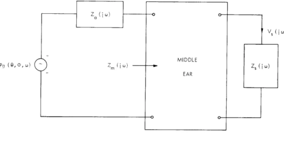
(This result is analogous to Bode's Resistance Integral theorem, 2 and follows at once from integrating Z(1/) around the right-half a-plane). Now consider the equivalent circuit (voltage ~ pressure, current ~ volume velocity) for the mechanical parts of the ear shown in Fig. XII-1. Here, Zm(jc) is the acoustic impedance (fundamental mode) looking into the middle ear from a point just external to the drum membrane; Z a(jw) and the pressure source Pg(O,

4,

w) represent the Thdvenin equivalent circuit looking outward into the ear canal for an incident plane sinusoidal acoustic wave of (rms)

zo (iW) 0

I vS (i W) MIDDLE

Pg ( 9, , W) Zm ( i) - - Z (iz )

EAR

Fig. XII- 1. Equivalent circuit.

pressure P, frequency

w

= ZTrf, and the propagation direction determined by 0 and

p

[g(0,

4,

w) is closely related to the acoustic cross section of the ear and head3]; and Vs (jwc) is the (rms) volume velocity of the stapes which, when driving the cochlea, is presumed to present a load impedance, Zs(jw), to the middle-ear mechanism.

To make use of (1), let Z (juo) Z (jw)

Z(jw) = (2)

z

a

(j)

+

Zm (j)

At low frequencies it is easy to show3 that mass effects dominate in the radiation impedance Za(jw); i. e., Za(jw) -

ju

L a. Since Z (jw) is a driving-point impedance, it follows that, for low frequencies,

Z(jw) - jwL, (3)

where L < L ._a The real part of Z(jw) is then constrained by (1).

(3)

Finally, it follows from conservation of energy and the positive-real-function char-acter of driving-point impedances that

Pg(O, 4, 1) Pg(O,

4,

R)

Z(jow)

2 Re [Z(ju)] > I Re [Zm(jc)] > Vs(j)I Re [Zs(j ], (4)

Z (jw) Z (jw)+Z (jow) 1 2

where equality holds between the first two terms if Za(jw) is lossless (i. e., Re [Za(j')]

0), and between the last two terms if the middle-ear system is lossless except for Zs (j)). Combining (1) and (4), we obtain

2 O V s(jL) K(w) du

<

i, (5) 0 Pg(O, , ) where

2 Z

Za(jw)

2

Re [Z (jw)

K(u) =

2 (6)

rcw L a

The inequality (5) is our principal result.

The significance of (5) depends sharply on the extent to which it is an approximate equality. Equality holds in (5) if the entire middle-ear system is lossless (except for

Z s(jw)), if Im [Za(jw)] >> Re [Z (jw)], and if Z (jw) is not zero at w = 0. There is some a

3,4 reason to believe that these are reasonable assumptions for the living ear. If (5) is an approximate equality, then, since K(w) is not a function of any middle-ear param-eter if Re [Zs(jw)] is attributed to the inner ear, improvements in transmission of the middle-ear system at one frequency through changes in middle-ear parameters would imply proportionate reductions (but not necessarily equal reductions if K(W) f constant) at some other frequency. From model studies, K(w) appears to be approximately con-stant for low frequencies up to nearly the frequency (~3-3. 5 kHz) of the quarter-wavelength resonance of the external ear. Near 3-3. 5 kHz, K(w) has a sharp peak. The

implications of this gain-bandwidth theorem, both for normal and pathological cases, will be discussed in a later report.

W. M. Siebert References

1. E. G. Wever and M. Lawrence, Physiological Acoustics (Princeton University Press, Princeton, N. J., 1954), Chap. 5.

2. H. W. Bode, Network Analysis and Feedback Amplifier Design (D. Van Nostrand Company, New York, 1945). 3. W. M. Siebert, "Simple Model of the Impedance Matching Properties of the External Ear," Quarterly Progress Report No. 96, Research Laboratory of Electronics, M. I. T., January 15, 1970, pp. 236-242.

4. A. R. Moller, "An Experimental Study of the Acoustic Impedance of the Middle Ear and Its Trans-mission Properties," Acta Oto-Laryngol. 60, 129-1 (1965).

(4)

B. _{ORGANIZATION OF THE POSTERIOR RAMUS AND GANGLION}

OF THE VIIIth CRANIAL NERVE OF THE BULLFROG

RANA CATESBEIANA

The VIIIth cranial nerve of the bullfrog is known to consist of anterior and posterior

rami with their cell bodies of origin in the anterior and posterior ganglia, respectively.

Within the otic capsule each ramus divides into four branches that project to separate

sensory organs. As described in an earlier paper, 1 branches of the anterior ramus

innervate the saccular and utricular maculae, and the anterior and lateral canal cristae.

Branches of the posterior ramus innervate the basilar and amphibian papillae, lagenar

macula, and posterior canal crista. Study of the anatomy of the posterior ramus has

disclosed new details of its organization.

1. Methods

a. Bullfrogs (Rana catesbeiana) were perfused with formalin. The otic capsules

with VIIIth nerve and (in some cases) medulla attached were dissected. Specimens were

stained in toto by the Sudan Black B method of Rasmussen

2

_{and decalcified.}

The wall

of the capsule, portions of the membranous labyrinth, and connective tissue were

care-fully removed, leaving the nerves and sensory epithelia. The bundle of nerve fibers

to each end-organ could then be teased away from the rest of the nerve. In this way

the nerve bundles were separated through the ganglion and along the nerve to the medulla,

thereby making it possible to determine the relative positions of the separate branches.

The branches could also be detached and whole mounted on slides for more detailed

study.

b.

_{Serial sections of the ear and VIIIth nerve in horizontal and cross-sectional}

planes

3

_{were studied to confirm the results of dissections. The location and extent of}

the VIIIth nerve ganglia, and, where possible, of the subganglia comprising them were

determined.

c.

_{Axonal degeneration techniques were employed. The posterior ramus was}

sec-tioned medial to the ganglion. The animals were sacrificed after one to two weeks and

the fibers were traced in the medulla using the Fink- Heimer modification of the Nauta

silver method

4

for staining degenerating axons.

2. Results

Each branch of the posterior ramus is a separate nerve traceable from end-organ

through the ganglion to the medulla. Examination of whole mounts of dissected branches

reveals little gross damage to individual nerve fibers; this suggests that there is little

or no interweaving of fibers from different branches.

As each nerve branch enters the ganglion it flattens into a band lying in a

(5)

dorsorostral to ventrocaudal plane.

The ganglion cells of the nerve to the amphibian

papilla lie most dorsal and slightly caudal (Fig. XII-2).

The cell bodies of origin of

the nerves to the posterior vertical canal crista, basilar papilla, lagenar macula and

SAC.

P.C.

A.P.

ANT.

/

I.SAP.C.

P.C.

B.P.

A.P.

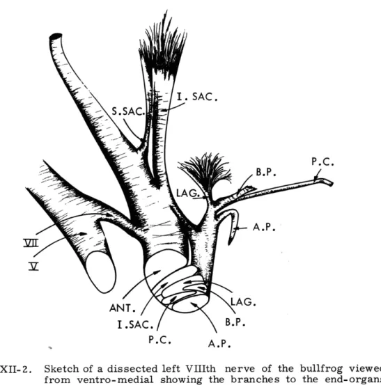
Fig. XII-2.

Sketch of a dissected left VIIIth nerve of the bullfrog viewed

from ventro-medial showing the branches to the end-organs

and their relative positions just medial to the ganglion.

V

=

fifth cranial nerve; VII

=

seventh cranial nerve; S. SAC. =

superior saccular nerve; ANT.

=

anterior ramus; I. SAC.

=

inferior saccular nerve; LAG.= lagenar nerve; B.P.=

basilar papilla nerve; P. C.

=

posterior canal nerve; A. P. =

amphibian papilla nerve.

inferior portion of the saccular macula lie successively more ventral in the posterior

ganglion. The inferior saccular nerve courses along the caudal face of the anterior

ramus, with which it runs distally, and crosses just outside the capsule wall to its cells

of origin in the posterior ganglion. The smaller superior saccular nerve courses

medi-ally with the anterior ramus. The ganglia of the auditory (i. e., basilar and amphibian)

papillae lie lateral to the nerve cell bodies of the other branches of the posterior ramus.

QPR No. 99

- I -- I r

-- ---181

(6)

(XII. COMMUNICATIONS BIOPHYSICS)

DORSAL

OPT. L.

\ \"

, \

"

,

CER.

MP.C. A.P. O. SAC.I B.P.

(II/"/

!f

!

!;

'

';

.

SiT-

LAG.

ROSTRAL

i

t

i

HYP.

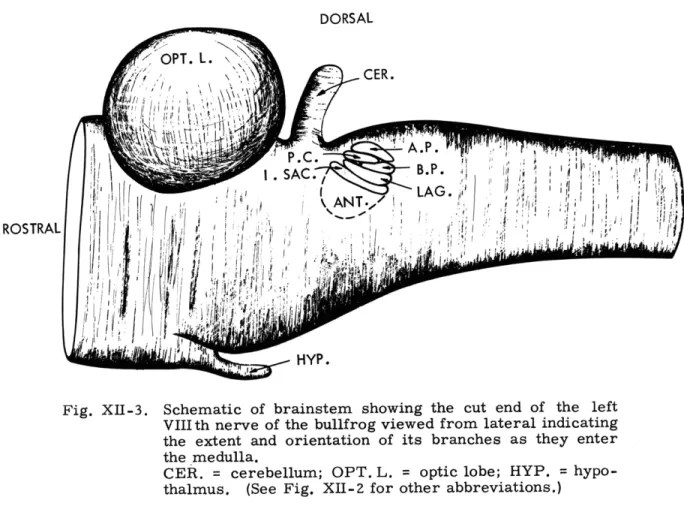
Fig. XII-3.

Schematic of brainstem showing the cut end of the left

VIIIth nerve of the bullfrog viewed from lateral indicating

the extent and orientation of its branches as they enter

the medulla.

CER. = cerebellum; OPT. L.

=

optic lobe; HYP. =

hypo-thalmus.

(See Fig. XII-Z for other abbreviations.)

Proximal to the ganglion, the nerve branches maintain their relative positions until

they enter the brainstem (Fig. XII-3).

Preliminary study of the results of axonal degeneration methods show that some of

the fibers of the posterior ramus terminate within the small-celled dorsal and some

within the large celled ventral nuclear complexes in the medulla.

R. L. Boord, L. B. Grochow, L. S. Frishkopf

(Professor Robert L. Boord is in the Biology Department of the University of Delaware.)

References

1. C. D. Geisler, W. A. van Bergeijk, and L. S. Frishkopf, "The Inner Ear of the

Bullfrog," J. Morph. 114, 43-58 (1964).

2. G. L. Rasmussen, "A Method of Staining the Statoacoustic Nerve in Bulk with Sudan

Black B," Anat. Rec. 139, 465-468 (1961).

3. G. L. Rasmussen, M. M. Powers, and G. Clark, "A Simple and Reliable Trichrome

Stain," J. Neuropathol. and Exper. Neurol. 4, 189-192 (1945).

4. R. P. Fink and L. Heimer, "Two Methods for Selective Silver Impregnation of

Degenerating Axons and Their Synaptic Endings in the Central Nervous System,"

Brain Res. 4, 369-374 (1967).

QPR No. 99

I -- I I r I ~ re

-c~

(7)

C. AUDITORY-NERVE FIRING PATTERNS FOR REPETITIVE PSEUDO NOISE-BURST STIMULI

Studies of the firing patterns of auditory-nerve fibers have been conducted with a 1-4

variety of acoustic stimuli. In particular, data have been published for tones, brief pulses (clicks), wideband random noise, and various combinations of these stimuli

(two-5 tones, paired clicks, tone and noise). Post stimulus-time (PST) histograms for clicks and tones show a stable time structure of responses. Click responses are syn-chronized to oscillations at the characteristic frequency (CF) for fibers with CF less than approximately 5 kHz, and the time pattern of responses to low-frequency simple tones shows a fine structure that is synchronized to the stimulating waveform. Tone bursts have a transient variation in the envelope of the PST histogram in addition to the fine structure. The envelope variation has a time constant of the order of 10 ms, and presumably reflects some kind of adaptation effect. When noise bursts are used as stimuli, the PST histograms (using the onset time of the bursts as reference) have about the same envelope shapes as the corresponding histograms for tone bursts. The time synchrony of responses to the fine structure is not evident, however, since these histograms are averaged over responses to different, nonperiodic waveforms. It is not clear a priori what the expected pattern of the fine structure should be because some wide-band stimuli (e. g., tone complexes2,' 3 and paired clicks4) result in complicated response patterns that are not predicted by simple extrapolations of models for single tones or clicks.

Because of the importance of the details of the time synchrony of responses for auditory-nerve models and because of the interesting psychoacoustic results for binaural detection of signals in noise, a crude, preliminary investigation of the time pattern of responses to wideband, noiselike stimuli was conducted in

collaboration with Dr. N. Y. S. Kiang at the Eaton- Peabody Laboratory for Audi-tory Physiology. The preparation and experimental procedure were the same as those described previously by Kiang, I the only difference being in the method

of generating the stimulus. In addition to using clicks and tones, a computer-generated noise burst was presented repetitively. In this way, PST histograms

of the responses to the pseudo-random noise burst could be generated, so that the time locking of the responses to the details of the wideband waveform could be investigated. The stimulus was generated by a computer (Digital Equipment

Corporation PDP-8) modified slightly to allow use of the accumulator and link as a 13-bit shift register that shifted every 9.75 s. This produces a very wideband waveform that, when filtered, has many characteristics of a sample

of random noise.6 The signal was lowpass-filtered with a 10-kHz cutoff and presented in 10 per second bursts of 50 ms duration; every burst was the same,

(8)

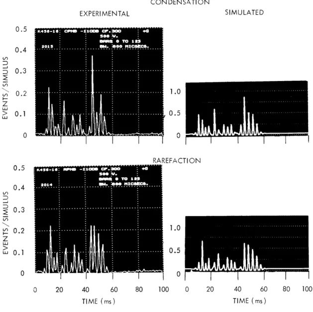
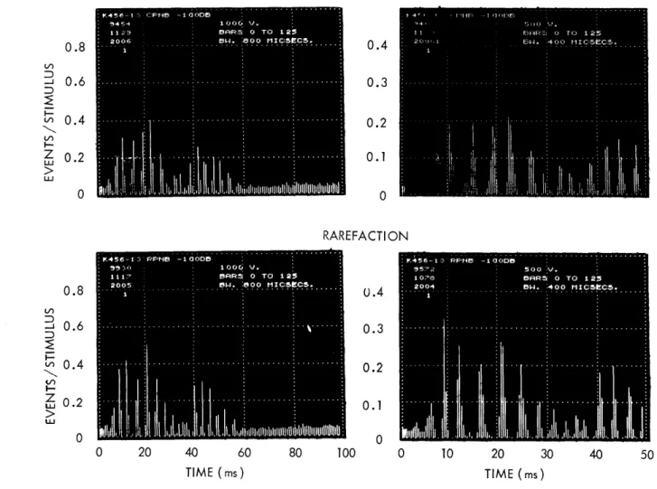
since the register was reset to the same initial value before each burst. The pseudo-noise signal, the starting pulses, and the neural responses were recorded on magnetic tape for later processing. PST histograms resulting from the same pseudo-noise burst are shown at the left in Figs. XII-4, XII-5, and XII-6, for fibers with several characteristic frequencies. The histograms show results for both polarities of the stimulus, consistently (but arbitrarily) labeled "Condensation" ("CPNB") for positive stimuli and "Rarefaction" ("RPNB") for negative stimuli. These histograms are interpolated versions of standard bar histograms. For comparison, bar histograms for fiber K456-13 (Fig. XII-5) are shown in Fig. XII-7. The bar histograms on the left correspond to the same bin width as the inter-polated histograms on the left in Fig. XII-5. Interpolated histograms are pre-sented to facilitate comparison with the simulation results that are shown on the right in Figs. XII-4, XII-5, and XII-6 and that are discussed below. For

each fiber the noise level was chosen to be approximately 20 dB above the "threshold" for that fiber. (Indicated levels are dB relative to 25 mV rms at the earphone.)

The detailed time structure of the responses to the stimulus is well illus-trated by the histograms. It is evident that the fine structure of the responses has a frequency that corresponds roughly to the CF of the unit. The indicated

CF were determined from the separation of the peaks in the PST histogram of responses to clicks; this sometimes gave disagreements of tens of cycles with the CF as determined on-line with tones during the experiments. Variations in envelope and phase are present in all histograms and can be seen to depend upon characteristic frequency. Note that the bin widths of the histograms in Figs. XII-4 and XII-5 are 800 i's. This is not sufficiently small compared with variations in the data to allow precise reproductions of the amplitudes of the individual peaks. Bar histograms with smaller bin widths are shown on the right in Fig. XII-7 and can be compared with the corresponding histograms on the left. This set, which corresponds to Fig. XII-5, was chosen because it shows the largest changes. _{The fiber corresponding to Fig. XII-6 has the highest} character-istic frequency (z500 Hz); the 800-

ps

bin width for this fiber resulted in larger discrepancies when compared with bin widths of 400 and 200

p.s,

and a bin width of 400 jps was chosen for this fiber.

In general, _{the interpolated PST histograms for these fibers resemble the} waveform obtained by passing the noise bursts through narrow-band filters (cen-tered in frequency near the CF of the respective fibers) followed by a rectifier. This observation is not unexpected on the basis of results for simple tones and clicks, since the PST histograms for these stimuli can be described by the

(9)

CONDENSATION EXPERIMENTAL SIMULATED

1.0

0.5

0.4

0.3

0.2

0.1

0

0.5

0.4

0.3

0.2

0.1 r

Ur

I

RAREFACTION

1.0

0.5

I I I I

1 I

I I I I I 0 20 40 60 80 100 0 20 40 60 80 100 TIME (ms) TIME (ms)

Fig. XII-4. PST histograms for responses to pseudo-noise bursts. Experimentally determined histograms are shown on the left; simulated histograms are shown on the right of the corresponding experimental histograms. Char-acteristic frequency of the fiber is approximately 340 Hz. (Note that the horizontal scales are different for left and right columns and that the vertical scale on the right is arbitrary.)

QPR No. 99

I

(10)

CONDENSATION EXPERIMENTAL 0.8 -0.6 -0.4 -0.2 -I I I I I SIMULATED 1.0 0.5 0 I I RAREFACTI ON 1.0 -0.5 -0 20 40 60 TIME (ms) Fig. XII-5. 80 100 I I I I 1 1 0 20 40 60 80 100 TIME (ms)

PST histograms for responses to pseudo-noise bursts.

Experimentally determined histograms are shown on the left; simulated histograms are shown on the right of the corresponding experimental histograms. Char-acteristic frequ en cy of the fiber is approximately 285 Hz. (Note that the horizontal scales are different for left and right columns and that the vertical scale on the right is arbitrary.)

QPR No. 99

0.2

:K456-13 RP1415 -11300B V. BRR5. 0 TO 1 2!5 2005 BW. :800 MICSIM5. ... ... . ...... ... ...... ...... . 0.8 0.6 0.4 186

(11)

CON

DENSATI ON

EXPERIMENTAL

0.5

0.4

0.3

0.2

0.1

0

0.5

0.4

0.3

0.2

0.1 SIMULATED

1.0

0

_.

5

RAREFACTION

1.0

0.5 I

I

0

10

20

30

40

50

0

10

20

30

40

50

TIME (ms) TIME (ms)

Fig. XII-6. PS'r histograms for responses to pseudo-noise bursts. Experimentally determined histograms are shown on the left; simulated histograms are shown on the right of the corresponding experimental histograms. Char-acteristic frequ en cy of the fiber is approximately 465 Hz. (Note that the horizontal scales are different for left and right columns and that the vertical scale on the right is arbitrary.)

(12)

CONDENSATION

800 ps BIN WIDTH

400 ps BIN WIDTH

K 4 54 -1 l C-.F1l - • 3 iiI 1 ,,,5

...

RAREF/ 0~ 20 4 0 V.10 200,5IM ( ms )ms80

0.4

0.3

0.2

0.1

0 ACTION

0.4

0.3

0.2

0.1

0

10

20

3

TIME (ms)

Fig. XII-7. Bar PST histograms for fiber K456-13 in response to pseudo-noise bursts. Left histograms have a bin width of 800 4s. Right histograms have a bin width of 400 is.

(Note that vertical scales also differ between the columns.)

QPR No. 99

0.8

-- 0.6

t;

0.4

Ln

I-Z

0.2

LU

0

0.8

- 0.6

n

0.4 I-t

0.2

0

40

50

188

(13)

general relation

r = A[s(t)

* h(t)] exp

_{r = A[s(t) h(t) exp}

_{+ F[s(t) * h(t)]}

**(t) * h(t)**

where the asterisk indicates convolution; h(t) is the impulse response of a narrow-band

filter centered at the characteristic frequency of the unit; s(t) is the stimulus, and F and

A are slowly varying (10-ms time constant) functionals of s(t) * h(t).

By choosing A

to be a constant equal to the spontaneous rate of firing and F a lowpass filtered envelope

of its argument, Siebert

7

has fitted the PST histograms for clicks (impulses) as a

func-tion of intensity for a fiber with low characteristic frequency (-500 Hz).

Equation 1 then

reduces to

±Sh(t)

r = A xp

SF[h(t)]

2)

where S is the amplitude of the click stimulus, the plus sign is used for a condensation

click, and the minus sign for a rarefaction click. Evans

8

has shown that the PST

histo-grams for responses to low-frequency tones can be well described in the form

r = A exp{g cos (wt-O)},

(3)

where A, g, and 0 are functions of stimulus amplitude and frequency

w.

This is again

a special case of Eq. 1. When tone bursts are used as stimuli, it is necessary to allow

A and g to vary slowly (also consistent with Eq. 1) to show the transient effects at the

beginning and end of the bursts. Applying Eq. 1 to noise bursts n(t) and ignoring the

variations, in A and F during the stimulus, we obtain the expression

r

=

A exp{±g[n(t)

*

h(t)]},

(4)

where A and g are constants.

With these motivations a crude test of the fit of Eq. 4 to the PST histograms from

this experiment was made.

Equation 4 was simulated with h(t) determined to

approxi-mate the click-response PST histogram at low intensity.

(According to Eq. 2, at low

intensities the PST histogram is described approximately by exp{Sh(t)} and can thus be

related to h(t).) The same shift-register sequence as used above was generated (not in

real time) on a different computer (Digital Equipment Corporation PDP-4) and digitally

filtered by convolving the noise sequence with the functions h(t).

The resulting

wave-forms were exponentiated to give the functions shown at the right of the PST histograms

for each fiber and each polarity (plus sign for condensation, minus sign for rarefaction)

in Figs XII-4, XII-5 and XII-6.

(14)

The simulated histograms agree relatively well with the observed data from these experiments. _{The position and spacing of the peaks, changes corresponding to the} polarity of the stimulus, and comparisons between histograms for fibers with different

characteristic frequencies are all consistent. The relative peak heights also show good agreement, even though this aspect of the simulated pattern is most sensitive to the spe-cific choice of the filter impulse response h(t), and even though the relative peak heights in the experimental histogram are somewhat affected by our choice of bin width. Note also that the approximation of constant A and g in Eq. 4 changes the relative heights to some degree; in fact, other results of the simulation study show that Eq. 1 describes the data better than Eq. 4. For example, it is obvious that the AGC action of the denominator of the exponent would increase the relative size of the first few peaks in the simulated histograms and would result in a better fit to the data in every case shown, especially for those shown in Fig. XII-5.

The results of this experiment offer limited support for the hypothesis that the PST histograms in response to some wideband stimuli can be approximated by the form in Eq. 1. The results are also consistent with the recent work of de Boer 9

that is based upon crosscorrelation of the input waveform with the spike train on a single auditory-nerve fiber when the input is a random-noise waveform. The rate function in Eq. 1, however, cannot describe the results of Pfeiffer and Goblick4 (who studied responses of auditory-nerve fibers to stimulation with multiple clicks). Their results cannot be explained by a linear filter followed by a nonlinearity. Similarly, paired-tone data2, 3 are dramatically inconsistent with the simple formulation in Eq. 1. It is clear that further work is required to separate those stimuli for which Eq. 1 is a good

approxi-mation to the PST histogram from those stimuli for which the histogram cannot be described by Eq. 1. One possible hypothesis that might be investigated, for example, is that Eq. 1 may be a good approximation for wideband stimuli whenever the spectrum does not contain multiple maxima.

H. S. Colburn References

1. N. Y. S. Kiang, T. Watanabe, Eleanor C. Thomas, and Louise F. Clark, Discharge Patterns of Single Fibers in the Cat's Auditory Nerve, Research Monograph 35 (The M. I. T. Press, Cambridge, Mass., 1965).

2. M. B. Sachs and N. Y. S. Kiang, "Two-Tone Inhibition in Auditory-Nerve Fibers," J. Acoust. Soc. Am. 43, 1120-1128 (1968).

3. J. L. Goldstein and N. Y. S. Kiang, "Neural Correlates of the Aural Combination Tone 2fl -f2," Proc. IEEE 56, 981-992 (1968).

4. T. J. Goblick, Jr., and R. R. Pfeiffer, "Time-Domain Measurements of Cochlear Non-linearities Using Combination Click Stimuli," J. Acoust. Soc. Am. 46, 924-938 (1969). 5. G. L. Gerstein and N. Y. S. Kiang, "An Approach to the Quantitative Analysis of

Electrophysiological Data from Single Neurons," Biophys. J. 1, 15-28 (1960).

(15)

6. D. Zierler, "Linear Recurring Sequences," J. Soc. Industr. Appl. Math. 7, 31

(1959).

7. W. M. Siebert (Private communication from material to be published).

8. J. E. Evans, "Time Pattern of Responses of Single Fibers in the Cat's Auditory Nerve to Continuous Tones" (Private communication from material to be published). 9. E. de Boer, "Correlation Studies Applied to the Frequency Resolution of the

Cochlea," J. Auditory Res. 7, 209-217 (1967).

(16)