Design and Operation of a Last Mile Transportation
System
By
Hai Wang
B.S., Civil Engineering, Tsinghua University (2009)
S.M., Transportation, Massachusetts Institute of Technology (2012) S.M., Operations Research, Massachusetts Institute of Technology (2012)
Submitted to the Sloan School of Management in partial fulfillment of the requirements for the degree of
Doctor of Philosophy in Operations Research at the
MASSACHUSETTS INSTITUTE OF TECHNOLOGY June 2015
© 2015 Massachusetts Institute of Technology. All Rights Reserved.
Signature of Author... Sloan School of Management
May 15th, 2015 Certified by ...
Amedeo R. Odoni Professor of Aeronautics and Astronautics and of Civil and Environmental Engineering Thesis Supervisor
Certified by ... Cynthia Barnhart Chancellor, Professor of Civil and Environmental Engineering Thesis Supervisor
Accepted by ... Patrick Jaillet Professor of Electrical Engineering and Computer Science Co-Director, Operations Research Center
Design and Operation of a Last Mile Transportation System
By
Hai Wang
Submitted to the Sloan School of Management on May 15, 2015, in partial fulfillment of the
requirements for the degree of
Doctor of Philosophy in Operations Research
Abstract
The Last Mile Problem refers to the provision of travel service from the nearest public transportation node to a home or office. Last Mile Transportation Systems (LMTS) are critical extensions to traditional public transit systems. We study the LMTS from three perspectives.
The first part of this thesis focuses on the design of a LMTS. We study the supply side of LMTS in a stochastic setting, with batch demands resulting from the arrival of groups of passengers at rail stations or bus stops who request last-mile service. Closed-form bounds and approximations are derived for the perClosed-formance of LMTS as a function of the fundamental design parameters of such systems. It is shown that a particular strict upper bound and an approximate upper bound perform consistently and remarkably well. These expressions can therefore be used for the preliminary planning and design of Last Mile Transportation Systems.
The second part of the thesis studies operating strategies for LMTS. Routes and schedules are determined for a multi-vehicle fleet of delivery vehicles with the objective of minimizing the waiting time and riding time of passengers. A myopic operating strategy is introduced first. Two more advanced operating strategies are then described, one based on a metaheuristic using tabu search and the other using an exact Mixed Integer Programming model, which is solved approximately in two stages. It is shown that all three operating strategies greatly outperform the naïve strategy of fixed routes and fixed vehicle dispatching schedules.
The third part presents a new perspective to the study of passenger utility functions in a LMTS. The unknown parameters of a passenger utility function are treated as unobserved events, and the characteristics of the transportation trips made by the passengers are treated as observed outcomes. We propose a method to identify the probability measures of the events given observations of the frequencies of outcomes by introducing the concept and assumptions of the Core Determining Class. We introduce a
combinatorial algorithm in which the noise in the observations data is ignored and a general procedure in which data noise is taken into consideration.
Thesis Supervisor: Amedeo R. Odoni
Title: Professor of Aeronautics and Astronautics and of Civil and Environmental Engineering
Thesis Supervisor: Cynthia Barnhart
5
Acknowledgements
First and foremost, I would like to express my deepest gratitude to my advisor Prof. Amedeo Odoni for everything he has done for me. In the past six years, he has been a constant source of knowledge, guidance, support and encouragement. I have benefited significantly from his immense knowledge, inspiration and patience. He always provides strong support, sound advice and tremendous guidance. I would not have come this far without him. He is the greatest mentor I have ever met or even heard of. His kindness and caring have made my journey at MIT a very pleasant one. He is an exceptional role model for me and it is my great honor to be one of the last group of PhD students working with him.
I would like to express my sincere appreciation to my advisor Prof. Cynthia Barnhart. Throughout the past three years, she has provided me with sound advice, insightful suggestions and lots of new ideas. Her broad perspective, high professional standards, and emphasis on the balance and combination of theory and practice have had a huge influence on me. This thesis would not have been possible without her. I am extremely fortunate to have Cindy as my advisor and I always feel I am very lucky to be working with her.
I would like to thank Prof. Patrick Jaillet, who also served on my thesis committee, for his valuable feedback, insightful suggestions and comments at various stages of my dissertation research. More importantly, he has been providing kind help ever since my early days as an MST student in MIT.
Additionally, this thesis has benefited from discussions with a number of members of MIT’s faculty: Prof. Dimitris Bertsimas, Prof. Andreas Schulz, Prof. Juan Pablo, and Prof. Jinhua Zhao. Chapter 4 of this thesis is a result of collaborating with Mr. Ye Luo from the Department of Economics of MIT. I also thank Prof. Richard Larson and Prof. Arnold Barnett. It was an amazing experience to work with them as a teaching assistant for the course of Urban Operations Research. I learnt much from their professionalism.
I am very grateful to Maria Marangiello, Laura Rose, and Andrew Carvalho for their administrative assistance. This dissertation has been supported by the MIT Chyn Duog
6
Shish Memorial Fellowship and the Future Urban Mobility program of the Singapore-MIT Alliance for Research and Technology (SMART).
Many thanks go to my friends at ORC and MIT. I have been extremely lucky to be surrounded by a group of peers who are individually brilliant, yet exceptionally supportive of each other. The friends here made my stay at MIT much more enjoyable and memorable. I would also like to thank all my Chinese friends in the Boston and Cambridge area, who created a home-like atmosphere for me in my best age.
Last, but not least, I would like to dedicate this thesis to my parents – my father Zhengqing Wang and my mother Suqing Xu. They provide unconditional love and endless support all the time. They are my everything and I owe my deepest gratitude to them.
7
Contents
List of Figures ... 11 List of Tables ... 13 Chapter 1 ... Introduction ... 151.1 Introduction and Literature Review ... 15
1.2 Thesis Outline and Contributions ... 18
Chapter 2 ... Design of a Last Mile Transportation System... 21
2.1 Background ... 21
2.2 Problem Description and Assumptions ... 23
2.3 Description of Overall Approach ... 25
2.4 The Unit-Capacity, Multi-Vehicle LMP ... 27
2.4.1 General Upper Bound and Approximation ... 28
2.4.2 Cyclic Assignment Policy ... 31
2.4.3 Another Approximation ... 34
2.4.3 Numerical Experiments for the Unit-Capacity, Multi-Vehicle LMP ... 37
2.5 General-Capacity, Multi-Vehicle LMP: Approximations ... 40
2.5.1 Adjustment of the Queueing Model ... 40
2.5.2 Approximating the Expected Value of Customer Service Times ... 41
2.5.3 Approximating the Variance of Customer Service Times ... 45
2.5.4 Simulation and Comparisons for the General-Capacity, Multi-Vehicle LMP ... 46
2.5.5 Relaxation Time ... 51
2.5.5 Another Test ... 53
2.6 Conclusion ... 54
Chapter 3 ... Operation of a Last Mile Transportation System ... 57
3.1 Introduction ... 57
3.2 Problem Description ... 59
3.3 Myopic Operation ... 62
3.3.1 Procedure of Myopic Operation ... 62
3.3.2 Myopic Formulation ... 67
8
3.4 Tabu Search ... 69
3.4.1 Notation and Attributes ... 70
3.4.2 Neighborhood Exploration ... 71
3.4.3 Tabu List ... 75
3.4.4 Evaluation of Moves and Aspiration Criteria ... 75
3.4.5 Termination Conditions ... 77
3.4.6 Tabu Search Algorithm ... 77
3.5 Mixed Integer Programming Formulation ... 78
3.5.1 Exact MIP model ... 79
3.5.2 First Stage: Solve MIP to the Level of Inter-arrival Time ... 81
3.5.3 Second Stage: Column Generation in the Original Formulation ... 83
3.6 Computational Study ... 84
3.6.1 Settings of Test Instances ... 85
3.6.2 Conventional Service with Fixed Routes and Schedules ... 86
3.6.3 Results and Discussion ... 88
3.7 Conclusion ... 93
Chapter 4 ... A New Perspective to Study Passenger Utility Functions – Core Determining Class: Construction, Approximation and Inference ... 95
4.1 Overall Approach ... 96
4.2 Example of Bipartite Graph ... 98
4.3 Core Determining Class ... 101
4.4 Exact Core Determining Class ... 105
4.5 A General Selection Procedure and Sparse Assumption ... 111
4.5.1 General Selection Procedure ... 111
4.5.2 Sparse Assumptions ... 114
4.6 Properties of the Selection Procedure with Application in the Core Determining Class Problem ... 117
4.6.1 General Properties ... 117
4.6.2 Application in Estimating Measure 𝑣 in the Core Determining Class Problem ... 122
4.7 Conclusion ... 127
Chapter 5 ... Concluding Remarks ... 129 Appendix A ...
9
Proofs in Chapter 4 ... 133
A.1 Proof of Lemma 4.2 ... 133
A.2 Proof of Theorem 4.1... 135
A.3 Proof of Lemma 4.4 ... 136
A.4 Proof of Theorem 4.2... 136
A.5 Proof of Theorem 4.3... 137
A.6 Proof of Lemma 4.7 ... 138
A.7 Proof of Lemma 4.8 ... 141
11
List of Figures
Figure 1.1 Schematic of a Last Mile Transportation System (LMTS) ... 16
Figure 2.1 Customer destinations and vehicles routes of the Unit-Capacity, Multi-Vehicle LMP 26 Figure 2.2 Customer destinations and vehicles routes of the General-Capacity, Multi-Vehicle LMP ... 27
Figure 2.3 Customer flow in the pre-assignment policy ... 29
Figure 2.4 Cyclic assignment policy ... 31
Figure 2.5 Waiting time component ... 34
Figure 2.6 Simulation results, bounds and approximations of average waiting time when 𝑛 = 20 ... 37
Figure 2.7 Simulation results, bounds and approximations of average waiting time when 𝑛 = 40 ... 38
Figure 2.8 Simulation results, bounds and approximations of average waiting time when 𝑛 = 60 ... 38
Figure 2.9 Simulation results, bounds and approximations of average waiting time when 𝑛 = 80 ... 39
Figure 2.10 Best routes for a 𝑗 = 40, 𝑐 = 10 instance (left), a 𝑗 = 40, 𝑐 = 4 instance (right) ... 43
Figure 2.11 Simulation and analytical results when 𝑐 = 5 𝑎𝑛𝑑 𝑛 = 40 ... 47
Figure 2.12 Simulation and analytical results when 𝑐 = 5 𝑎𝑛𝑑 𝑛 = 80 ... 48
Figure 2.13 Simulation and analytical results when 𝑐 = 5 𝑎𝑛𝑑 𝑛 = 120 ... 48
Figure 2.14 Simulation and analytical results when 𝑐 = 10 𝑎𝑛𝑑 𝑛 = 40 ... 48
Figure 2.15 Simulation and analytical results when 𝑐 = 10 𝑎𝑛𝑑 𝑛 = 80 ... 49
Figure 2.16 Simulation and analytical results when 𝑐 = 10 𝑎𝑛𝑑 𝑛 = 120 ... 49
Figure 2.17 Simulation and analytical results when 𝑐 = 15 𝑎𝑛𝑑 𝑛 = 120 ... 49
Figure 2.18 Simulation and analytical results when 𝑐 = 20 𝑎𝑛𝑑 𝑛 = 120 ... 50
Figure 2.19 Schematic LMTS around crossroad ... 54
Figure 3.1 Schematic of a Last Mile Transportation System with LM stops ... 57
Figure 3.2 Examples of feasible route and infeasible route... 60
Figure 3.3 Procedure of myopic operation ... 64
Figure 3.4 Evaluation procedure for solution 𝑠 in tabu search ... 77
Figure 3.5 Route type selected in the first stage ... 84
Figure 3.6 Route types of decision variables generated in the second stage ... 84
12
Figure 3.8 Passenger waiting time and riding time fo 𝐽 = 15, 𝑁 = 30, 𝑐 = 6, 𝑚 = 5 ... 92
Figure 3.9 Vehicle service time and number of trips for 𝐽 = 15, 𝑁 = 30, 𝑐 = 6, 𝑚 = 5 ... 92
Figure 4.1 Example of a bipartite graph ... 101
Figure 4.2 Correspondence mapping of an example ... 109
13
List of Tables
Table 2.1 Error of expression (2.18) compared to results of simulation ... 44
Table 2.2 Upper bound and approximation of relaxation time 𝑡3 ... 53
Table 3.1 Procedure of myopic operation ... 63
Table 3.2 Example of myopic operation ... 66
Table 3.3 Notation for myopic formulation ... 67
Table 3.4 Evaluation procedure for solution 𝑠 in tabu search ... 76
Table 3.5 Tabu search algorithm ... 78
Table 3.6 (Additional) Notation for the exact MIP model ... 79
Table 3.7 (Additional) Notation for the first stage model ... 82
Table 3.8 Demand intensity at LM stops ... 86
Table 3.9 (Additional) Notation for bus line design for conventional service ... 87
Table 3.10 Results for 𝐽 = 10, 𝑁 = 15, 𝑐 = 6, 𝑚 = 3 ... 88
Table 3.11 Results for 𝐽 = 10, 𝑁 = 15, 𝑐 = 6, 𝑚 = 7 ... 88
Table 3.12 Results for 𝐽 = 15, 𝑁 = 30, 𝑐 = 6, 𝑚 = 5 ... 89
Table 3.13 Results for 𝐽 = 15, 𝑁 = 30, 𝑐 = 6, 𝑚 = 7 ... 89
15
Chapter 1
Introduction
1.1 Introduction and Literature Review
The Last Mile Problem (LMP) refers to the provision of travel service from a public transportation node to home or workplace (“last mile”) or vice versa (“first mile”). This public transportation node could be the nearest rapid transit rail station or a stop of a scheduled bus line. The unavailability of this type of service is one of the main deterrents to the use of public transport in urban areas, especially for certain demographic groups, such as schoolchildren, seniors and people with certain physical handicaps. Currently, the default solutions to the LMP are walking, riding a bike, taking a taxi, or driving a private vehicle.
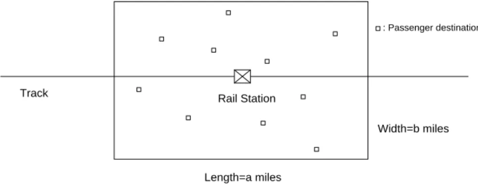
A conceptual Last Mile Transportation System (LMTS) is described schematically in Figure 1.1, which shows an urban area surrounding a public-transit rail station, where trains arrive and discharge passengers. The passengers’ final destinations (homes, apartments, offices and workplaces) are distributed in the area. A fleet of vehicles transports these passengers to their eventual destinations (or locations which are very close to their eventual destinations) and empty vehicles return to the station to pick up waiting passengers or newly arriving ones. We describe the specific setting of LMTS in more detail in Chapter 2 and Chapter 3, in the context of system design and system operation, respectively.
16
Figure 1.1 Schematic of a Last Mile Transportation System (LMTS)
Many issues must be addressed when designing and operating a LMTS. On the supply side, it is essential to deal with difficult questions concerning the stochastic aspects of the system; additionally, operating strategies addressing vehicle routing and scheduling, and passenger service assignment are needed to support system operations. The demand side requires an understanding and estimation of the potential LMTS loads as a function of demographic characteristics, nature of trip, level of service, time-of-day, cost, etc. The LMTS loads can be partially estimated through a study of passenger utility functions.
An extensive literature in this general area has generated various models for a number of application contexts related to the LMP with early work dating back to the 1960s. We mention here only a few that are among the most influential in the field or especially relevant to the approach we have adopted. Many references specific to the individual topics studied are provided, respectively, in Chapters 2, 3, and 4.
Several influential papers in the Operations Research literature have addressed problems with significant similarities to the LMP. The Dynamic Traveling Repairman Problem (DTRP) was introduced in two papers by Bertsimas and Van Ryzin. They consider the DTRP in the cases of a single-vehicle “fleet” (1991) and of multiple vehicles (1993). The Dynamic Pick-up and Delivery Problem (DPDP) was studied by Swihart and Papastavrou (1999), who derived bounds on the performance of several DPDP variants for light and heavy traffic. The Car Pooling Problem (CPP), introduced by Baldacci et al. (2004), also has features similar to the LMP – or, more exactly, to the First
Width=b miles
Length=a miles Rail Station
: Passenger destination
17
Mile Problem. The paper presents both exact and heuristic methods for solving the CPP based on integer programming formulations.
Many more recent papers deal with last mile supply chains and freight last mile systems in the age of booming e-commerce. The related literature has been growing rapidly in the last 15 years, including Lee and Whang (2001), Punakivi et al. (2001), Esper et al. (2003), Balcik et al. (2008), Boyer et al. (2009), and Song et al. (2009). For example, Balcik et al. (2008) consider a vehicle-based last mile distribution system geared to the needs of humanitarian relief chains. They propose a mixed integer programming model to determine delivery schedules for vehicles and to allocate resources equitably in the face of certain types of constraints. Boyer et al. (2009) examine the effects of two factors, customer density and delivery window length, on the overall efficiency of “last mile routes” for package deliveries. As for passenger last mile systems, some case studies provide analysis of LMTS in different contexts, such as the study of a bicycle-sharing program for an LMTS in Beijing by Liu et al. (2012).
Personal rapid transit (PRT), which refers to a variety of transportation systems with characteristics similar in some ways to the last mile transportation system studied in this thesis, has also attracted significant attention in recent years. Papers considering PRT systems from a range of perspectives (all different from those presented here) include those by Anderson (1998), Bly and Teychenne (2005), Lees-Miller et al. (2009, 2010), Berger et al. (2011), and Mueller and Sgouridis (2011).
Finally, a large number of papers have dealt with the Dial-a-Ride Problem (DARP) and related variations – see, e.g., Jaw et al. (1986), Lei et al. (2012). A good critical review of the DARP literature by Cordeau and Laporte (2007) underlines, among other points, the fact that this body of work does not address well some of the queueing aspects of the subject systems – a deficiency that Chapter 2 tries to remedy.
It should also be noted that similarities exist between the LMP and various queuing, dispatching, routing, scheduling, service assignment, and resource allocation problems arising in entirely different contexts such as the design of manufacturing systems, the operation of elevator banks, and the scheduling of school-bus systems. The major
18
difference between the LMP and the more “traditional” problems is that, in the LMP, passengers (service requests) arrive in (possibly large) batches, not singly. This difference, however, makes the analysis of LMP much more difficult analytically than the analysis of these other problems.
1.2 Thesis Outline and Contributions
The main body of this thesis is organized as follows.
In Chapter 2, we study the supply side of the last mile transportation system in a stochastic setting, with stochastic batch demands resulting from the arrival of groups of passengers who request last-mile service at urban rail stations or bus stops. The main contribution of this chapter is the derivation of several closed-form expressions that approximate the principal performance characteristics of last mile transportations systems as a function of the fundamental design parameters of such systems. An initial set of results is obtained for the case in which a fleet of vehicles of unit capacity provides the Last Mile service and each delivery route consists of a simple round-trip between the rail station or bus stop and a single passenger’s destination. These results are then extended to the general case in which the capacity of a vehicle is a small number (up to 20). It is shown through comparisons with simulation results that the approximations perform consistently well for a broad and realistic range of input values and conditions. These expressions can therefore be used for the preliminary planning and design of last mile transportation systems, especially for determining approximately resource requirements, such as the number of vehicles/servers needed to achieve some pre-specified level of service, as measured by the expected waiting time until a passenger is picked up from the station or delivered to her destination.
In Chapter 3, we consider the operation of a last mile transportation system with batch demands. The main contribution of this chapter is the development of operating strategies and algorithms for the design of passenger delivery schedules and vehicle routes for a multi-vehicle fleet of delivery vehicles with the objective of minimizing the waiting time and riding time of passengers. A myopic operating strategy is introduced first, for the
19
case in which the last mile demand from each group of arriving passengers is revealed sequentially. Two more advanced operating strategies are then described in detail, one based on a metaheuristic using tabu search and the other using an exact Mixed Integer Programming (MIP) model, which is solved approximately in two stages. These operating strategies are implemented in a number of computational experiments with a broad and realistic range of inputs values and conditions. It is shown that: the myopic strategy performs well for certain ranges of the input values and poorly for others; the tabu search metaheuristic provides solutions of good quality in a reasonably short computational time; and the MIP model provides the best solutions, but has greatly increased computational requirements. Thus the best approach to the routing and scheduling of the LMTS fleet depends on the context and the user’s needs.
In Chapter 4, we present a novel approach to the study of the passenger utility function in a last mile transportation system. The passenger utility function provides critical information to LMTS service providers when it comes to understanding and estimating passenger demand and designing and operating their systems. From our new perspective, which is significantly different from existing ones, the unknown parameters in the passenger utility function are treated as unobserved events (defined in detail in Chapter 4), and the specific characteristics of transportation trips, such as passenger waiting time, vehicle travel time and monetary travel cost that can be collected in the real data, are considered as observed outcomes (defined in detail in Chapter 4). In this chapter, given a bipartite graph representing the relations between events and outcomes, we develop a combinatorial algorithm to identify irredundant linear inequalities to bound the probability measures of events using observations of the frequencies of the outcomes. We then extend the irredundant linear inequality identification problem and propose a general inequality selection procedure in which we take the data noise of the outcome observations into consideration. The primary model, which is similar to the Dantzig Selector in the 𝑙1-regularization problem, is a linear programming formulation motivated
by Farkas’ lemma. It measures the importance of each linear inequality among an entire set of numerous inequalities under sparse assumptions. The novel approach presented in Chapter 4 calibrates the possible set of the unknown parameters in the passenger utility
20
function and is helpful in understanding and estimating passenger demand for last mile transportation systems.
Finally, in Chapter 5 we conclude with a summary of the thesis and discuss several directions for future research.
21
Chapter 2
Design of a Last Mile Transportation System
The focus of this chapter is on the stochastic analysis of the supply side of LMTS: given a probabilistic description of demand, design a LMTS that operates under dynamic and stochastic conditions according to certain guidelines and satisfies a set of Level of Service (LOS) requirements. This implies specifying such system characteristics as vehicle fleet size, service frequency, vehicle dispatching strategies, vehicle routing strategies, monitoring and control of operations, etc. We propose several closed-form expressions as functions of system parameters to bound and estimate system performance, such as the average passenger waiting time and the average passenger riding time. The analytical expressions derived herein can be very useful in designing LMTS, specifically in determining resource requirements for these systems, such as how many vehicles would be necessary to achieve a specified level of service (as measured by expected time until a passenger boards a vehicle or is delivered to his/her destination) and how many kilometers per day these vehicles would travel.
2.1 Background
Bounding and approximating the performance of a last mile transportation system is difficult analytically, as the planning and management of a LMTS generally involves such complications as: stochastic travel times; batch arrivals of prospective passengers; partitioning of demands among vehicles; routing of the vehicles; queueing issues; and,
22
obviously, numerous considerations concerning staffing and economic sustainability. With the exception of staffing and economic issues, these complications are addressed in this chapter in a static setting.
In a general LMTS, passengers arrive in batches, not singly. Moreover, the size of these batches is a random variable. Queueing systems with batch arrivals are notoriously difficult analytically. A further complication is that the “service times” of passengers are determined by the length (or the duration) of the routes traveled by each vehicle. Thus, in designing a LMTS, it is necessary to consider simultaneously the problems of: allocating passengers among vehicles; routing the vehicles and estimating the lengths of the routes; and computing the queueing performance characteristics of the system.
The main body of this chapter is organized as follows. In Section 2.2, we describe in detail the version of the LMP that we are studying and discuss the associated fundamental assumptions. Section 2.3 outlines our overall approach: we begin by deriving a set of queueing results by considering a fleet of vehicles with capacity for a single passenger (𝑐 = 1) and then extend the analysis by allowing the vehicle capacity to be arbitrary and by incorporating the resulting travel time estimates into the queueing expressions derived for the 𝑐 = 1 case. Section 2.4 presents our analysis and results for the unit-capacity case. We derive an upper bound and an approximate expression for the performance of a LMTS as a function of its design parameters and then show through a set of simulation experiments that the resulting estimates approximate well the observed waiting times. Section 2.5 examines the general capacity case (𝑐 > 1) by, first, proposing approximate analytical expressions for the expected value and the variance of the travel times associated with fleets consisting of vehicles with general capacity, and then applying these expressions to the queueing approximation derived in Section 2.4. The results again compare well with those obtained from simulations. We also show that the relaxation time of the queue in the LMTS is significantly shorter than the duration of the time intervals during which the respective demand rates for an LMTS system can be approximated as being roughly constant. It is therefore reasonable to use the steady state approximations derived in this chapter. Section 2.6 contains a summary and concluding remarks.
23
2.2 Problem Description and Assumptions
We now describe in more detail the LMP scenario of Figure 1.1. The LMTS operates as follows: let STA be the transit rail station served by the LMTS. Consider a passenger, PAX, who boards a train at any station (“ORIGIN”) for the purpose of traveling to STA and will then board a LMTS vehicle for transport to her home. PAX is required to provide advance notice to LMTS of her impending arrival at STA. The time interval between the advance notice and the actual arrival of PAX at STA is of the order of several minutes (e.g., at least 5 or 10 minutes) to give the LMTS system sufficient time to plan the service of PAX. In practical terms, the advance notice could be generated by PAX in a number of alternative ways. For example, PAX could use a smart-phone when she arrives at ORIGIN or when she enters her train to STA; or, she could tap a smart card on a special-purpose screen, as she is entering ORIGIN or while aboard the train. The resulting message to the LMTS includes the expected time of arrival of PAX at STA (easy to predict, once the passenger is at the ORIGIN station or aboard a train) and her ultimate destination, e.g., her home address. If the great majority of LMTS users are subscribers whose home addresses are pre-registered, then the only information that PAX will have to provide will be an identification number or code.
Once the information about PAX is received the LMTS will assign PAX to one of the vehicles of the LMTS fleet, plan the route of that vehicle so it includes a visit to the ultimate destination of PAX, estimate the departure time of the vehicle from STA, and notify PAX accordingly. PAX will receive a message (on her smart-phone or by tapping her card on a screen when she arrives at STA) that indicates the vehicle she has been assigned to and the planned departure time of the vehicle from STA (e.g., “please board Vehicle 123 which will depart from STA at 4:26 PM”). Once all the passengers assigned to a vehicle are on board, the vehicle will execute a delivery route, visiting the destination of each of the passengers and will then return to STA to pick up the passengers for its next delivery tour.
24
The LMTS described above possesses the generic system features that we are most interested in: arrivals of passengers in “batches” (groups) at STA; clustering of passengers into subgroups for assignment to a fleet of vehicles; routing of the vehicles to deliver the passengers on board; and a requirement for fast computation of waiting times and other performance parameters so that, for example, passengers can be notified in a timely way of the departure time of the vehicle they have been assigned to. Actual implementations would probably involve some simpler variants of the above features.
Given the service region’s geometry, passenger demand, the spatial distribution of the passenger destinations, and the number, capacity and travel speed of the LMTS vehicles, examples of performance metrics that we wish to compute include: the average waiting time until boarding a vehicle, the average riding time of passengers, the average waiting time until delivery, the minimum number of vehicles we need to reach stable operation, vehicle productivity and workload, and eventually (but not in this thesis) the general cost of operating the system and the service vs. cost trade-offs involved.
We now identify briefly the specifics of the model considered. With reference to Figure 2.1, we make the following assumptions: (i) headways, ℎ, between arrivals of trains at the station (and discharges of passengers) are constant; (ii) passengers are discharged in batches after each train’s arrival; (iii) the batch size is a general random variable, 𝑁, with known expectation 𝐸(𝑁) = 𝑛 and variance 𝑉𝑎𝑟(𝑁) = 𝜎𝑁2; (iv) all
passengers arriving in a single batch request service essentially simultaneously; (v) given the size of any particular batch, 𝑁 = 𝑁0, the destinations of the 𝑁0passengers in the batch
are distributed identically, uniformly and independently in a service region; (vi) the service region is convex and compact with known dimensions; (vii) the delivery fleet (or pick-up fleet, in the case of “First Mile” service) consists of 𝑚 vehicles, each with integer capacity, 𝑐.
We believe that these assumptions are sufficiently general for approximating, to a first order, the characteristics of many potential variations of LMTS. Note that our model includes the most difficult, from the analytical point of view, features that one might encounter in an LMTS: batch arrivals, stochastic demand, stochastic service times, and the presence of queueing phenomena interfaced with clustering and routing problems.
25
2.3 Description of Overall Approach
Sections 2.4 and 2.5 of the chapter describe in detail our analysis and results. In this section we provide a brief description of the overall approach we have followed to provide perspective for these detailed sections. We have adopted a viewpoint under which the LMTS is regarded as a spatially distributed queueing system. In line, with typical queueing terminology, we shall refer henceforth to passengers as “customers”. The 𝑚 parallel servers (the vehicle fleet) serve customers in groups of 𝑐 or smaller, where 𝑐 is the capacity of each vehicle. The service time for each group is equal to the travel time associated with a vehicle tour that begins at the station/depot, visits each of the 𝑐 (or fewer) customer destinations and returns to the station/depot to pick up a new group.
Because queueing systems with batch arrivals (like the arrivals of customers at STA) and batch services (like the service of groups of customers by each vehicle) are difficult to analyze, we resort to a two-step approach. In Step 1, we assume that 𝑐 = 1, i.e., that the delivery vehicles have unit capacity. Thus,service times consist simply of the duration of a round-trip between STA and one customer’s destination (Figure 2.1), with the destination being randomly and uniformly distributed within the service area per our assumption (v) in Section 2.2. In this way, we obtain a 𝐷𝑁/𝐺/𝑚/∞ queueing system in queueing theory notation, where 𝐷𝑁 indicates batch arrivals at constant (“Deterministic”) intervals with the number of arriving customers in each batch described by random variable 𝑁; 𝐺 denotes the fact that the distribution of service times (i.e., the duration of the round trips between STA and customer destinations) is “general”; and 𝑚 and ∞ indicate, respectively, the number of servicevehicles and the fact that no a priori limit is placed on the number of customers waiting for pickup at STA.
26 Width=b miles Length=a miles Rail Station : Passenger destination Track
Figure 2.1 Customer destinations and vehicles routes of the Unit-Capacity, Multi-Vehicle LMP
As no closed-form expressions are available for the fundamental quantities that describe the performance of a 𝐷𝑁/𝐺/𝑚/∞ system, we then attempt to obtain expressions for similar queueing systems, which are more tractable mathematically. Through a series of simplifications, we derive (i) an upper bound and (ii) an approximate expression for the mean waiting time associated with 𝐷𝑁/𝐺/𝑚/∞ queues. We then carry out an extensive set of simple simulation experiments and conclude that these expressions provide good estimates of the performance of the system (with 𝑐 = 1) under a broad range of system design parameters.
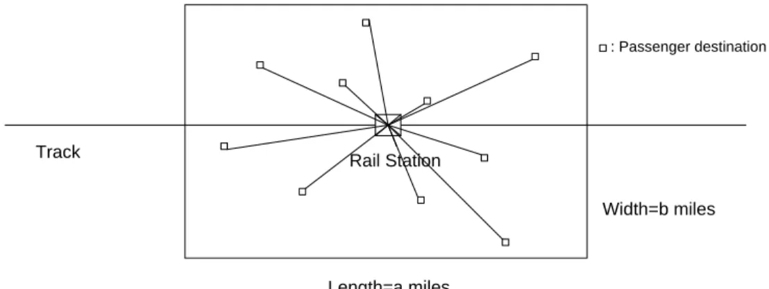
Step 2 examines the general case, in which service times are equal to the duration of delivery tours consisting of 𝑐(> 1) or fewer delivery stops, as shown in Figure 2.2. To apply to the general capacity case the queueing expressions that were derived in Step 1, we need to partition the customers, design near-optimal tours/routes for the vehicles, and compute the approximate expectation and variance of the vehicle tour length. We accomplish this by using arguments from geometrical probability and from the literature on the Traveling Salesman Problem and Vehicle Routing Problem. We then use these expressions, along with the queueing-based approximation derived in Step 1, to complete the process of estimating the performance of the LMTS for the general case of arbitrary fleet size and arbitrary vehicle capacity. Finally, we compare again our approximate estimates to the results of a series of simulations over a broad range of input values.
27
Figure 2.2 Customer destinations and vehicles routes of the General-Capacity, Multi-Vehicle LMP
2.4 The Unit-Capacity, Multi-Vehicle LMP
In this section we present the analysis of the case described in Section 2.3 as Step 1, in which 𝑐 = 1, and 𝑚 is an arbitrary positive integer. As already indicated (Figure 2.1), the length of the vehicle trips in this case is equal to two times the distance between the rail station and a customer’s destination. If we postulate constant and unit travel speed, the expressions for travel times are identical with those derived for travel distances.
The basic notation is summarized as follows:
ℎ = the constant headway between arrivals of trains (and discharges of customers) at
the station STA;
𝑁 = a random variable denoting the number of LMTS customers (“batch size”) discharged after the arrival of a train at STA, with the sizes of successive batches being mutually independent, and 𝐸(𝑁) = 𝑛 and 𝑉𝑎𝑟(𝑁) = 𝜎𝑁2 denoting, respectively, the
expectation and variance of 𝑁;
𝜆𝑎= the arrival rate of customer batches (= 1/ℎ);
𝜎𝑎2= the variance of the inter-arrival time of customer batches (𝜎𝑎2= 0 for constant
headways); Width=b miles Length=a miles Rail Station : Passenger destination Track
28
𝑆 = a random variable denoting the service time of a random LMTS customer with 𝐸(𝑆) = 𝑠 and variance 𝑉𝑎𝑟(𝑆) = 𝜎𝑆2.
Note that the successive service times of any given vehicle in the fleet are independent and identically distributed. The traffic load (or utilization ratio) is given by 𝜌 = 𝑛𝑠/ℎ𝑚, since 𝑚/𝑠 is the service rate of the LMTS, while 𝑛/ℎ is the rate of customer arrivals per unit of time.
We are particularly interested in the expected waiting time, 𝑊𝑞, of LMTS customers
until they board one of the 𝑚 vehicles to be transported to their eventual destination. Determining this expected waiting time as a function of the LMTS design parameters is a critical step toward developing the means to design LMTS satisfying certain level-of-service requirements.
2.4.1 General Upper Bound and Approximation
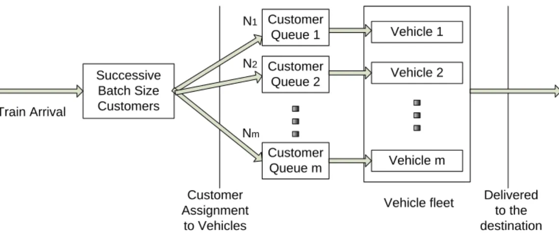
We begin by obtaining a general upper bound and approximate expression for 𝑊𝑞 in the
original Unit-Capacity, Multi-Vehicle 𝐷𝑁/𝐺/𝑚/∞ model. To do this, for each train’s arrival, we pre-assign the discharged customers to different vehicles and then construct a corresponding single-server queueing model 𝐷𝑁𝑆/𝐺/1/∞ for each vehicle, where 𝑁𝑆is the
random variable indicating the number of customers from any single train assigned to the same vehicle. Each customer can be served only by the vehicle to which she has been pre-assigned.
With such an assignment policy, service inefficiencies will exist since a customer is required to wait for his or her assigned vehicle, even when other vehicles may be available. Thus, the average waiting time in this case will be larger than the average waiting time in the original model. The customer flow is shown schematically in Figure 2.3.
29
Figure 2.3 Customer flow in the pre-assignment policy
The 𝐷𝑁𝑆/𝐺/1/∞ model is still difficult to work with. To obtain approximate
expressions for 𝑊𝑞, we decompose the problem into two parts. First, the 𝑁𝑆 customers in
a batch who are assigned to the same vehicle are treated as a single “macro-customer” 𝑃. If we only consider the “macro-customer”, this reduces the 𝐷𝑁𝑆/𝐺/1/∞ model to the
more tractable 𝐷/𝐺/1/∞ model and allows us to obtain an approximation for 𝑊𝑞1, the
expected waiting time until the first customer in 𝑃 receives service.
Let 𝑇 be the service time of the “macro-customer”, 𝑇 = ∑𝑁𝑖=1𝑆 𝑆𝑖, where 𝑁𝑆 depends on
the assignment policy and 𝑆1, 𝑆2, … , 𝑆𝑁are the service times of the real customers, which
are mutually independent and identically distributed. Note that 𝑁𝑆 is a random variable.
Therefore, 𝐸(𝑇) = ∑ 𝐸(𝑆𝑖) = 𝑁𝑆 𝑖=1 𝐸(𝑁𝑆)𝑠, 𝑉𝑎𝑟(𝑇) = 𝐸(𝑁𝑆)𝜎𝑆2+ 𝑠2𝑉𝑎𝑟(𝑁𝑆), 𝐶𝑇2=𝐸(𝑁𝑆)𝜎𝑆2+ 𝑠2𝑉𝑎𝑟(𝑁𝑆) 𝐸2(𝑁 𝑆)𝑠2
Additionally, 𝜎𝑎2= 0 because of constant “macro-customer” inter-arrival times, 𝜆𝑎= 1/ ℎ, 𝜌 = 𝐸(𝑇)/ℎ = 𝐸(𝑁𝑆)𝑠/ℎ. According to Kingman (1961), Kingman (1962), and Ott (1987), an upper bound for 𝑊𝑞1, the expected waiting time of 𝐷/𝐺/1/∞ queue is:
Vehicle m Vehicle 2 Vehicle 1 Successive Batch Size Customers Customer Assignment to Vehicles Delivered to the destination Vehicle fleet Train Arrival Customer Queue 1 Customer Queue 2 Customer Queue m N1 N2 Nm
30 𝑊𝑞1= 𝑊𝑞(𝐷/𝐺/1/∞) ≤𝜆𝑎(𝜎𝑎2+ 𝜎𝑇2) 2(1 − 𝜌) = 1 ℎ (0 + 𝑉𝑎𝑟(𝑇)) 2(1 −𝐸(𝑇)ℎ ) =𝐸(𝑁𝑆)𝜎𝑆2+ 𝑠2𝑉𝑎𝑟(𝑁𝑆) 2(ℎ − 𝐸(𝑁𝑆)𝑠) (2.1) According to Kraemer et al. (1976), an approximation of 𝑊𝑞1 is provided by: 𝑊𝑞1= 𝑊𝑞(𝐷/𝐺/1/∞) ≈ 𝑉𝑎𝑟(𝑇) 2(ℎ − 𝐸(𝑇))∙ exp [− 2(ℎ − 𝐸(𝑇))𝐸(𝑇) 3𝑉𝑎𝑟(𝑇) ] =𝐸(𝑁𝑆)𝜎𝑆 2+ 𝑠2𝑉𝑎𝑟(𝑁 𝑆) 2(ℎ − 𝐸(𝑁𝑆)𝑠) ∙ exp [− 2(ℎ − 𝐸(𝑁𝑆)𝑠)𝐸(𝑁𝑆)𝑠 3𝐸(𝑁𝑆)𝜎𝑆2+ 3𝑠2𝑉𝑎𝑟(𝑁 𝑆)] (2.2)
In a second step, we then compute the additional expected waiting time, 𝑊𝑞2, until
each of the individual customers in macro-customer 𝑃 receives service, following the service to the “macro-customer”. For the 𝑖 𝑡ℎ customer in 𝑃, we consider the additional expected waiting time due to being preceded by 𝑖 − 1 other customers in 𝑃. If the
macro-customer consists of 𝑘 customers and 𝑘 ≥ 1, the customer in the 𝑖 𝑡ℎ position suffers the expected additional total waiting time 𝑊𝑞,𝑖 𝑡ℎ= ∑𝑖−1𝑗=1𝑠𝑗= (𝑖 − 1)𝑠 , where 𝑠𝑗 is the
expected service time of the 𝑗 𝑡ℎ customer served before the 𝑖 𝑡ℎ customer. Let
𝑊𝑞,𝑘 𝑐𝑢𝑠𝑡𝑜𝑚𝑒𝑟𝑠 denote the expected total additional waiting time of the 𝑘 customers:
𝑊𝑞,𝑘 𝑐𝑢𝑠𝑡𝑜𝑚𝑒𝑟𝑠= ∑𝑘𝑖=1𝑊𝑞,𝑖 𝑡ℎ 𝑘 = ∑𝑘 (𝑖 − 1)𝑠 𝑖=1 𝑘 = (𝑘 − 1)𝑠 2 , 𝑘 ≥ 1
If 𝑘 = 0, no customers are served, so that 𝑊𝑞,0 𝑐𝑢𝑠𝑡𝑜𝑚𝑒𝑟 = 0. According to the Law of
Total Expectation, the expected additional waiting time of a customer is then given by:
𝑊𝑞2=∑ 𝑃(𝑘)𝑊𝑞,𝑘 𝑐𝑢𝑠𝑡𝑜𝑚𝑒𝑟𝑠𝑘 ∞ 𝑘=0 ∑∞ 𝑃(𝑘)𝑘 𝑘=0 =𝑠𝑉𝑎𝑟(𝑁𝑆) + 𝑠𝐸2(𝑁𝑆) − 𝑠𝐸(𝑁𝑆) 2𝐸(𝑁𝑆) (2.3)
Thus the upper bound we seek is:
𝑊𝑞 = 𝑊𝑞1+ 𝑊𝑞2 ≤𝐸(𝑁𝑆)𝜎𝑆2+ 𝑠2𝑉𝑎𝑟(𝑁𝑆) 2(ℎ − 𝐸(𝑁𝑆)𝑠) +
𝑠𝑉𝑎𝑟(𝑁𝑆) + 𝑠𝐸2(𝑁𝑆) − 𝑠𝐸(𝑁𝑆)
2𝐸(𝑁𝑆) (2.4)
31 𝑊𝑞 = 𝑊𝑞1+ 𝑊𝑞2 ≈𝐸(𝑁𝑆)𝜎𝑆 2+ 𝑠2𝑉𝑎𝑟(𝑁 𝑆) 2(ℎ − 𝐸(𝑁𝑆)𝑠) ∙ exp [− 2(ℎ − 𝐸(𝑁𝑆)𝑠)𝐸(𝑁𝑆)𝑠 3𝐸(𝑁𝑆)𝜎𝑆2+ 3𝑠2𝑉𝑎𝑟(𝑁𝑆)] +𝑠𝑉𝑎𝑟(𝑁𝑆) + 𝑠𝐸2(𝑁𝑆) − 𝑠𝐸(𝑁𝑆) 2𝐸(𝑁𝑆) (2.5)
Expression (2.4) and (2.5) are valid under general assumptions about the probability density functions of the batch size, 𝑁, and the service times, 𝑆. Moreover, (2.4) and (2.5)
have been derived without considering how exactly customers are assigned to vehicles. We next analyze one particular reasonable policy for customer assignment to vehicles. The policy will provide a modified 𝐷𝑁𝑆/𝐺/1/∞ model with 𝐸(𝑁𝑆) and 𝑉𝑎𝑟(𝑁𝑆), leading to
corresponding expressions for 𝑊𝑞1 and 𝑊𝑞2, and, ultimately, to an upper bound and an
approximation for 𝑊𝑞.
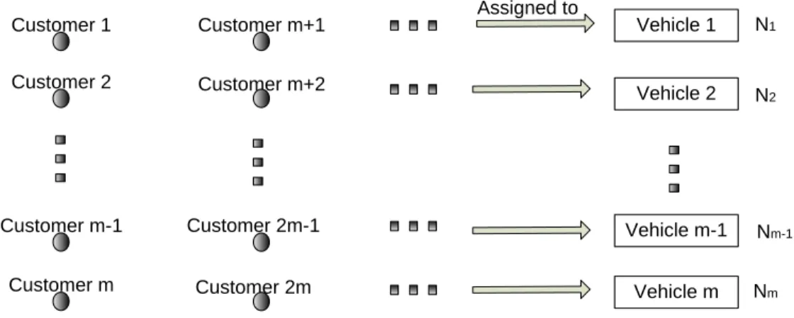
2.4.2 Cyclic Assignment Policy
One possible policy for allocating customers to vehicles is to assign customers in cyclic order to the vehicles: the first customer in the batch is assigned to Vehicle 1, the second to Vehicle 2, …, the (𝑚 + 1) 𝑡ℎ to Vehicle 1 again, and so forth. No jockeying of customers, after being assigned to vehicles, is allowed. Figure 2.4 illustrates this policy, which requires assigning an “identification number” to each vehicle to distinguish among them.
Figure 2.4 Cyclic assignment policy
Vehicle 1 Vehicle m Vehicle m-1 Vehicle 2 Customer m Customer m-1 Customer 2 Customer 1 Customer m+1 Customer 2m Customer 2m-1 Customer m+2 Assigned to N1 N2 Nm-1 Nm
32
We have a total of 𝑚 vehicles, labeled as “Vehicle 1”, “Vehicle 2”,…, “Vehicle 𝑚”. Let 𝑁𝑖 be the random variable indicating the number of customers assigned to “Vehicle i” after the arrival of a particular train, with the assignment process upon arrival of each train being independent of the arrival process upon arrival of any other train. When one train arrives, we order the 𝑚 vehicles in sequence: the vehicle that receives customers first is called “1st server”, the vehicle that receives customers second is called “2nd server”, etc. Let 𝑋𝑖 be the random variable indicating the number of customers assigned to the “𝑖 𝑡ℎ server” after the arrival of a particular train. Then,
𝑋1= ⌊ 𝑁 + 𝑚 − 1 𝑚 ⌋ , 𝑋2= ⌊ 𝑁 + 𝑚 − 2 𝑚 ⌋ , … , 𝑋𝑚−1= ⌊ 𝑁 + 1 𝑚 ⌋ , 𝑋𝑚= ⌊ 𝑁 𝑚⌋ 𝑁 = 𝑋1+ 𝑋2+ ⋯ + 𝑋𝑚−1+ 𝑋𝑚
If we order the vehicles randomly, the probability that Vehicle 𝑖 will become the 𝑗 𝑡ℎ server for some train is 1/𝑚. The modified model can be considered as 𝐷𝑁𝑖/𝐺/1/∞. Since
𝑁1, 𝑁2, … , 𝑁𝑚 are identically distributed, all 𝐷𝑁𝑖/𝐺/1/∞ models can be viewed as identical 𝐷𝑁𝑆/𝐺/1/∞ models although 𝑁
1, 𝑁2, … , 𝑁𝑚are not necessarily independent.
Recalling that 𝑁 is the random variable indicating the total number of customers coming from one train, let 𝑁 = 𝐾𝑚 + 𝑅, where 𝐾 = ⌊𝑁/𝑚⌋, and 𝑅 is the remainder after division of 𝑁 by 𝑚. We can therefore express 𝑁 as a 2-dimensional random vector, (𝐾, 𝑅). 𝑋𝑖 = {𝐾,𝐾 + 1,𝑅 + 1 ≤ 𝑖 ≤ 𝑚; 1 ≤ 𝑖 ≤ 𝑅; 𝐸(𝑁𝑆|(𝐾, 𝑅)) =𝑚1 [𝐸(𝑋1|(𝐾, 𝑅)) + 𝐸(𝑋2|(𝐾, 𝑅)) + … + 𝐸(𝑋𝑚|(𝐾, 𝑅))] = 𝑁 𝑚; 𝑉𝑎𝑟(𝑁𝑆|(𝐾, 𝑅)) = 𝑃(𝑁𝑆 = 𝐾 + 1)(𝐾 + 1 − 𝐸(𝑁𝑆|(𝐾, 𝑅)))2+ 𝑃(𝑁 𝑆= 𝐾)(𝐾 − 𝐸(𝑁𝑆|(𝐾, 𝑅)))2 = 𝑅 𝑚∙ (𝐾 + 1 − 𝐾𝑚 + 𝑅 𝑚 )2+ 𝑚 − 𝑅 𝑚 ∙ (𝐾 − 𝐾𝑚 + 𝑅 𝑚 )2= 𝑅𝑚 − 𝑅2 𝑚2 𝐸(𝑁𝑆) = 𝐸(𝐸(𝑁𝑆|(𝐾, 𝑅))) = 𝐸( 𝑁 𝑚) = 𝑛 𝑚
33 𝑉𝑎𝑟(𝑁𝑆) = 𝐸(𝑉𝑎𝑟(𝑁𝑆|(𝐾, 𝑅))) + 𝑉𝑎𝑟(𝐸(𝑁𝑆|(𝐾, 𝑅))) = 𝐸( 𝑅𝑚 − 𝑅2 𝑚2 ) + 𝑉𝑎𝑟( 𝑁 𝑚) =𝐸(𝑅𝑚 − 𝑅2) 𝑚2 + 𝜎𝑁2 𝑚2
Since 𝑅 < 𝑚, it is also true that 𝑅𝑚 − 𝑅2≤ 𝑚2/4, and
𝑉𝑎𝑟(𝑁𝑆) ≤1 4+ 𝜎𝑁2 𝑚2= 4𝜎𝑁2+ 𝑚2 4𝑚2
In practice, the number of customers 𝑁 from each batch will typically be much larger than the number of vehicles 𝑚, and the remainder 𝑅 will tend to be uniformly distributed in {0, 1, … , 𝑚 − 1}. Then,
𝐸(𝑅𝑚 − 𝑅2) ≈𝑚2− 1
6𝑚2 , 𝑉𝑎𝑟(𝑁𝑆) ≈
6𝜎𝑁2+ 𝑚2− 1 6𝑚2
By substituting the bound and approximation of 𝐸(𝑁𝑆) and 𝑉𝑎𝑟(𝑁𝑆) into (2.4) and
(2.5), respectively, the model corresponding to the cyclic assignment policy finally leads to the following upper bound and approximation for the case of a General service time distribution: 𝑊𝑞 ≤4𝑚𝑛 2(𝜎 𝑆2+ 𝑠2) − 4𝑛3𝑠2+ 4ℎ𝑚𝑠(𝜎𝑁2+ 𝑛2) + ℎ𝑚3𝑠 − 4ℎ𝑚2𝑛𝑠 8𝑚𝑛(ℎ𝑚 − 𝑛𝑠) (2.6) 𝑊𝑞 ≈6𝑚𝑛𝜎𝑆2+ 6𝑠2𝜎𝑁2+ 𝑚2𝑠2− 𝑠2 12𝑚(ℎ𝑚 − 𝑛𝑠) ∙ exp [− 4(ℎ𝑚 − 𝑛𝑠)𝑛𝑠 6𝑚𝑛𝜎𝑆2+ 6𝑠2𝜎 𝑁2+ 𝑚2𝑠2− 𝑠2 ] +(6𝜎𝑁 2+ 𝑚2+ 6𝑛2− 6𝑚𝑛 − 1)𝑠 12𝑚𝑛 (2.7)
Assuming the service area is a 𝑏 × 𝑏 square with the train station located at the square’s center, the travel metric is right angle, and the travel speed is constant throughout the service region and equal to 1, and for Poisson batch sizes, the bound (2.6) becomes:
𝑊𝑞 ≤
14𝑏2𝑚𝑛2+ 12𝑏ℎ𝑚𝑛2− 12𝑏2𝑛3+ 12𝑏ℎ𝑚𝑛 − 12𝑏ℎ𝑚2𝑛 + 3𝑏ℎ𝑚3
24𝑚𝑛(ℎ𝑚 − 𝑏𝑛) (2.8)
34 𝑊𝑞 ≈ (𝑚 + 6)𝑏2𝑛 + 𝑏2𝑚2− 𝑏2 12𝑚(ℎ𝑚 − 𝑏𝑛) ∙ exp [− 4(ℎ𝑚 − 𝑏𝑛)𝑛 𝑏𝑚𝑛 + 6𝑏𝑛 + 𝑏𝑚2− 𝑏] +(𝑚 2+ 6𝑛2+ 6𝑛 − 6𝑚𝑛 − 1)𝑏 12𝑚𝑛 (2.9) 2.4.3 Another Approximation
In addition to the approach described above, we have developed an alternative way to simplify and approximate the 𝐷𝑁/𝐺/𝑚 queue of the Unit-Capacity, Multi-Vehicle LMP.
As shown in Figure 2.5, in this alternative approximation, the waiting time is decomposed into two parts: 𝑊𝑞3, the waiting time until the first passenger in a batch
receives service; and 𝑊𝑞4, the waiting time until the following individual customers in that batch receive service. We treat all the customers from each arrival batch as a single “macro-customer” 𝑃′ and do not pre-assign them to vehicles. This reduces the 𝐷𝑁/𝐺/𝑚/
∞ model to the 𝐷/𝐺/𝑚/∞ model and allows us to obtain an approximation for 𝑊𝑞3 using approximations of the 𝐺/𝐺/𝑚/∞ model, such as those of Köllerström (1974) and Whitt (1993).
Wq3 Wq4
Time that a batch arrives at the
D/G/m queue
Time that the first passenger in the batch
get service
Average time that following passengers in
the batch get service
Figure 2.5 Waiting time component
The detailed derivation is described as follows.
Let 𝑇′ be the service time of the “macro-customer” 𝑃′, 𝑇′= ∑ 𝑆 𝑖 𝑁 𝑖=1 , then: 𝐸(𝑇′) = ∑ 𝐸(𝑆 𝑖) 𝑁 𝑖=1 = 𝑛𝑠, 𝑉𝑎𝑟(𝑇′) = 𝑛𝜎 𝑠2+ 𝑠2𝜎𝑁2, 𝐶𝑇2′ = 𝑛𝜎𝑠2+ 𝑠2𝜎𝑁2 𝑛2𝑠2
35
In addition, 𝜎𝑎2= 0, 𝜆𝑎= 1/ ℎ, 𝜌 = 𝐸(𝑇′)/𝑚ℎ = 𝑛𝑠/𝑚ℎ. According to Whitt (1994), a
good approximation for 𝐷/𝐺/𝑚/∞ queue can be written as: 𝑊𝑞3≈ 𝜙(𝑚, 𝜌)𝐶𝑇′ 2 2 𝑊𝑞(𝑀/𝑀/𝑚) where 𝜙(𝑚, 𝜌) = (1 − 4 ∙ 𝑚𝑖𝑛 {0.24,(1 − 𝜌)(𝑚 − 1) ((4 + 5𝑚) 1 2− 2) 16𝑚𝜌 }) ∙ 𝑒𝑥𝑝 ( −2(1 − 𝜌) 3𝜌 ) and 𝑊𝑞(𝑀/𝑀/𝑚) ≈ 𝐸(𝑇′)(𝜌(√2(𝑚+1)−1)) 𝑚(1 − 𝜌)
Therefore, substituting 𝐸(𝑇′), 𝑉𝑎𝑟(𝑇′), 𝐶𝑇2′ and 𝜌, we obtain:
𝑊𝑞3≈ (1 − 4 ∙ 𝑚𝑖𝑛 {0.24, (𝑚ℎ − 𝑛𝑠)(𝑚 − 1) ((4 + 5𝑚)12− 2) 16𝑚𝑛𝑠 }) ∙ 𝑒𝑥𝑝 ( −2(𝑚ℎ − 𝑛𝑠) 3𝑛𝑠 ) ∙ ∙ℎ ∙ (𝑛𝑠) (√2(𝑚+1)−2)∙ (𝑛𝜎 𝑠2+ 𝑠2𝜎𝑁2) 2 ∙ (𝑚ℎ)(√2(𝑚+1)−1)∙ (𝑚ℎ − 𝑛𝑠) (2.10)
Next we study 𝑊𝑞4. At the point in time when the first passenger in the batch gets
access to service, one server becomes available, while the other servers are still busy. Hence, the following passengers in the batch should wait for more available servers. We can approximate the expected waiting time until the next server becomes available as 𝑠/𝑚. Therefore, assuming 𝑘 passengers in the batch:
For the first passenger in the batch: 𝑊𝑞4,1𝑠𝑡= 0;
For the second passenger in the batch: 𝑊𝑞4,2𝑛𝑑= 𝑠/𝑚; For the third passenger in the batch: 𝑊𝑞4,3𝑟𝑑= 2𝑠/𝑚; …
36
For the 𝑘 𝑡ℎ passenger in the batch: 𝑊𝑞4,𝑘 𝑡ℎ= (𝑘 − 1)𝑠/𝑚;
Let 𝑊𝑞4,𝑘 𝑐𝑢𝑠𝑡𝑜𝑚𝑒𝑟𝑠 denote the average additional waiting time of the 𝑘 customers:
𝑊𝑞4,𝑘 𝑐𝑢𝑠𝑡𝑜𝑚𝑒𝑟𝑠=∑ 𝑊𝑞4,𝑖 𝑡ℎ 𝑘 𝑖=1 𝑘 = ∑𝑘𝑖=1(𝑖 − 1)𝑠/𝑚 𝑘 = (𝑘 − 1)𝑠 2𝑚 , 𝑘 ≥ 1
If 𝑘 = 0, no customers are served, so that 𝑊𝑞4,0 𝑐𝑢𝑠𝑡𝑜𝑚𝑒𝑟 = 0. According to the Law of Total Expectation, the expected additional waiting time of a customer is given by:
𝑊𝑞4= ∑∞𝑘=0𝑃(𝑘)𝑊𝑞4,𝑘 𝑐𝑢𝑠𝑡𝑜𝑚𝑒𝑟𝑠𝑘 ∑∞ 𝑃(𝑘)𝑘 𝑘=0 =𝑠𝑉𝑎𝑟(𝑁) + 𝑠𝐸 2(𝑁) − 𝑠𝐸(𝑁) 2𝑚𝐸(𝑁) = 𝑠𝜎𝑁2+ 𝑠𝑛2− 𝑠𝑛 2𝑚𝑛 (2.11)
Therefore, the approximation of the expected waiting time of passengers is obtained: 𝑊𝑞 ≈ 𝑊𝑞3+ 𝑊𝑞4 ≈ (1 − 4 ∙ 𝑚𝑖𝑛 {0.24,(𝑚ℎ − 𝑛𝑠)(𝑚 − 1) ((4 + 5𝑚) 1 2− 2) 16𝑚𝜆𝑠 }) ∙ 𝑒𝑥𝑝 (−2(𝑚ℎ − 𝑛𝑠) 3𝑛𝑠 ) ∙ ℎ ∙ (𝑛𝑠)(√2(𝑚+1)−2)∙ (𝑛𝜎𝑠2+ 𝑠2𝜎 𝑁2) 2(𝑚ℎ − 𝑛𝑠) ∙ (𝑚ℎ)(√2(𝑚+1)−1) + 𝑠𝜎𝑁2+ 𝑠𝑛2− 𝑠𝑛 2𝑚𝑛 (2.12)
Expression (2.12) is valid under general assumptions about the probability density functions of the batch size 𝑁, and the service times 𝑆. For Poisson batch sizes, a square service region with a right-angle distance metric, and vehicles with unit capacity and constant speed 1, the approximation (2.12) becomes:
𝑊𝑞 ≈ (1 − 4 ∙ 𝑚𝑖𝑛 {0.24, (𝑚ℎ − 𝑛𝑏)(𝑚 − 1) ((4 + 5𝑚)12− 2) 16𝑚𝑛𝑏 }) ∙ 𝑒𝑥𝑝 ( −2(𝑚ℎ − 𝑛𝑏) 3𝑛𝑏 ) ∙ 7𝑏ℎ 12(𝑚ℎ − 𝑛𝑏)∙ ( 𝑛𝑏 𝑚ℎ) (√2(𝑚+1)−1) + 𝑠𝑛 2𝑚 (2.13)
37
According to numerical experiments, these approximations (2.12) and (2.13) perform worse than the approximations (2.7) and (2.9) in most cases, except under extremely high utilization ratios when the system is unstable and both approximations perform poorly, anyway. Additionally, the expressions (2.7) and (2.9) are simple closed-form expressions, much simpler than expressions (2.12) and (2.13).
2.4.3 Numerical Experiments for the Unit-Capacity, Multi-Vehicle LMP
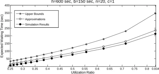
To assess the performance of the expressions obtained in Sections 2.4.1 and 2.4.2 under a broad range of conditions, a simple simulation of the Unit-Capacity, Multi-Vehicle LMP was carried out with a program written in java. We consider a square service region with geometry 𝑏/𝑣 = 2.5 𝑚𝑖𝑛 = 150 𝑠𝑒𝑐 , headway ℎ = 10 𝑚𝑖𝑛 = 600 𝑠𝑒𝑐 , and Poisson-distributed batch sizes of 𝑛 = 20, 40, 60, 80. We selected these parameters so that the system would make sense physically.
Figure 2.6 Simulation results, bounds and approximations of average waiting time when 𝒏 = 𝟐𝟎 0.250 0.3 0.35 0.4 0.45 0.5 0.55 0.6 0.65 0.7 0.75 0.8 0.834 50 100 150 200 250 300 350 400 Utilization Ratio E xp e ct e d W a it in g T im e ( se c) h=600 sec, b=150 sec, n=20, c=1 Upper Bounds Approximations Simulation Results
38
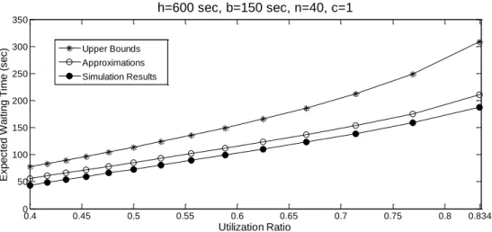
Figure 2.7 Simulation results, bounds and approximations of average waiting time when 𝒏 = 𝟒𝟎
Figure 2.8 Simulation results, bounds and approximations of average waiting time when 𝒏 = 𝟔𝟎 0.4 0.45 0.5 0.55 0.6 0.65 0.7 0.75 0.8 0.834 0 50 100 150 200 250 300 350 Utilization Ratio E xp e ct e d W a it in g T im e ( se c) h=600 sec, b=150 sec, n=40, c=1 Upper Bounds Approximations Simulation Results 0.5 0.55 0.6 0.65 0.7 0.75 0.8 0.85 0.883 50 100 150 200 250 300 350 400 450 500 Utilization Ratio E xp e ct e d W a it in g T im e ( se c) h=600 sec, b=150 sec, n=60, c=1 Upper Bounds Approximations Simulation Results
39
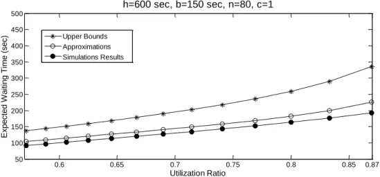
Figure 2.9 Simulation results, bounds and approximations of average waiting time when 𝒏 = 𝟖𝟎
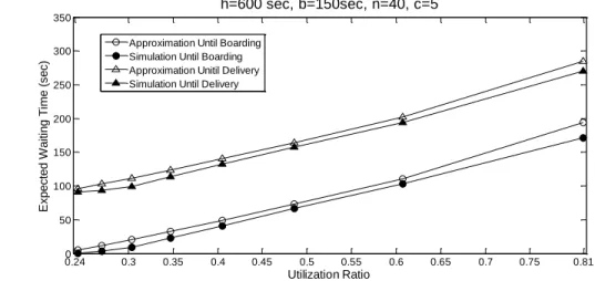
Figures 2.6 – 2.9 plot the simulation results and our estimates for the average waiting time per customer 𝑊𝑞 (in seconds) against the utilization ratio 𝜌 = 𝑠𝑛/ℎ𝑚. Since the
simulated system has Poisson customer batch size and a square service region, the upper bound (expression (2.8)), and the approximation (expression (2.9)) from Sections 2.4.2 are applicable and considered here. For each demand intensity 𝑛, the utilization ratio 𝜌 takes on a set of discrete values because the number of vehicles, 𝑚, is integer. We have plotted the points with utilization ratio less than 0.9, above which the system is highly unstable and the average waiting time is too long to be accepted practically.
It can be seen that (2.8) is a consistently reliable upper bound for 𝑊𝑞, while (2.9)
provides a very good approximation for the entire range of parameter values for which the LMTS remains stable. In a practical system, it would be desirable to achieve values of 1 to 5 minutes, for the average waiting time until customers board a vehicle. Note from Figures 2.6 – 2.9 that for this range of values (60 to 300 seconds) the difference between the approximation and the simulation results stays small in absolute or percentage terms. For example, when 𝑛 = 20 (Figure 2.6), this difference never exceeds the greater of 15 seconds or 12% for values of 𝑊𝑞 between 1 and 4 minutes.
We have also performed simulation experiments with rectangular and diamond-shaped service regions and with discontinuities in the travel medium, such as an
0.6 0.65 0.7 0.75 0.8 0.85 0.87 50 100 150 200 250 300 350 400 450 500 Utilization Ratio E xp e ct e d W a it in g T im e ( se c) h=600 sec, b=150 sec, n=80, c=1 Upper Bounds Approximations Simulations Results
40
impenetrable barrier to travel. For these environments we have derived expressions for 𝑊𝑞, analogous to (2.8) and (2.9), based on (2.6) and (2.7) – see Wang (2012). These experiments led to the conclusion that the analytical upper bound and approximation continue to perform well under a wide range of conditions.
2.5 General-Capacity, Multi-Vehicle LMP: Approximations
In this section we shall generalize the results of Section 2.4 by considering the General-Capacity, Multi-Vehicle LMP, in which the vehicle capacity, 𝑐, and the number of vehicles, 𝑚, are arbitrary positive integers. The vehicles will now travel along more complicated routes than in the 𝑐 = 1 case to deliver customers to their destinations. In practice, one would expect the vehicle capacity to be smaller than that of a regular bus – typically a number between 3, for service provided by taxi-like vehicles, and 20, for large vans.
As explained in Section 2.3, the General-Capacity, Multi-Vehicle LMTS will be viewed as a spatially distributed queueing system in which the service times are equal to the amount of time it takes to complete a customer delivery tour and return to the train station (Figure 2.2). After each batch of arrivals, the customers must be partitioned into clusters and assigned to vehicles according to their destinations and the vehicles must then be routed with the objective of obtaining a shortest total travel distance – which translates into shortest service times and smallest overall queueing. This means that the estimation of model parameters, such as the expected value and the variance of service times, is now far more complicated than when 𝑐 = 1.
2.5.1 Adjustment of the Queueing Model
We first need to make some adjustments to the principal expression (2.7) that we have derived from our queueing model. For the General (𝑐 > 1 ) Capacity case, General distribution of customer batch size and General service times, the approximation for the waiting time until boarding a vehicle is given by:
41 𝑊𝑞,𝐵𝑜𝑎𝑟𝑑≈ 6𝑚𝐸(𝑁𝐸)𝑉𝑎𝑟(𝑆𝐸) + 6𝐸2(𝑆 𝐸)𝑉𝑎𝑟(𝑁𝐸) + 𝐸2(𝑆𝐸)𝑚2− 𝐸2(𝑆𝐸) 12𝑚(ℎ𝑚 − 𝐸(𝑁𝐸)𝐸(𝑆𝐸)) ∙ 𝑒𝑥𝑝 [− 4(ℎ𝑚 − 𝐸(𝑁𝐸)𝐸(𝑆𝐸))𝐸(𝑁𝐸)𝐸(𝑆𝐸) 6𝑚𝐸(𝑁𝐸)𝑉𝑎𝑟(𝑆𝐸) + 6𝐸2(𝑆 𝐸)𝑉𝑎𝑟(𝑁𝐸) + 𝐸2(𝑆𝐸)𝑚2− 𝐸2(𝑆𝐸)] +(6𝑉𝑎𝑟(𝑁𝐸) + 𝑚2+ 6𝐸2(𝑁𝐸) − 6𝑚𝐸(𝑁𝐸) − 1)𝐸(𝑆𝐸) 12𝑚𝐸(𝑁𝐸) (2.14)
The expression (2.14) is exactly the same as (2.7), except 𝑆 is substituted by 𝑆𝐸, the
travel time to serve 𝑐 customers, and 𝑁 by 𝑁𝐸, the random variable indicating the number
of tours formed following the arrival of a batch of customers.
Note that in (2.14) we have used the notation 𝑊𝑞,𝐵𝑜𝑎𝑟𝑑 for the expected waiting time
until a customer will board a vehicle, while in (2.7) we used the notation 𝑊𝑞 for the same
quantity. This is because we also want to introduce here another quantity, 𝑊𝑅𝑖𝑑𝑖𝑛𝑔, which
is defined as the expected time a customer will spend riding on the vehicle before being delivered to her destination. Considering the riding component of the trip, the total expected time from the instant a customer arrives at the rail station until she is delivered at her destination is given by
𝑊𝐷𝑒𝑙𝑖𝑣𝑒𝑟𝑒𝑑 = 𝑊𝑞,𝐵𝑜𝑎𝑟𝑑+ 𝑊𝑅𝑖𝑑𝑖𝑛𝑔 (2.15) The expected riding time of the 𝑖 𝑡ℎ delivered customer in a tour with 𝑐 customer deliveries is approximated by 𝑖 × 𝐸(𝑆𝐸)/(𝑐 + 1) and the expected riding time of a random
customer is 𝐸(𝑆𝐸)/2.
2.5.2 Approximating the Expected Value of Customer Service Times
We turn next to the task of evaluating the performance of the general expressions (2.14) and (2.15). To do this, expressions must be developed for all terms involving 𝑆𝐸 and 𝑁𝐸. In this subsection and the next two, we propose a set of such approximate expressions for the case in which the destinations of the customers are uniformly and independently
42
distributed within a square 𝑏 × 𝑏 district, assuming Euclidean travel. An entirely different
operating environment is examined in Section 2.5.6.
We start with the critical quantity 𝐸(𝑆𝐸), the expected travel time to deliver 𝑐
customers. Consider the situation in which 𝑗 customers are to be delivered by vehicles with capacity 𝑐 each within the district of interest in a minimum total amount of travel time. Vehicles must return to their origin (the train station). This is a classical Vehicle Routing Problem (VRP).
Eilon et al. (1971) proposed an empirical formula for 𝐸(𝑇𝑉𝑅𝑇𝑗,𝑐), the total length of
vehicle routing tours when a total of 𝑗 customers are delivered using vehicles of capacity 𝑐, but tested it for only up to 𝑗 = 70 and 𝑐 = 10. Daganzo (1984) provided another simple and intuitive analytical approximation:
𝐸(𝑇𝑉𝑅𝑇𝑗,𝑐) ≈2𝑟𝑗𝑐 + 0.57√𝑗𝐴 (2.16)
where 𝑟 is the average distance between the customers and the depot and 𝐴 is the area of service region. For a 𝑏 × 𝑏 square region, uniformly distributed customer destinations, and the depot located at the center of the region, 𝑟 = 0.382𝑏 and expression (2.16) becomes:
𝐸(𝑇𝑉𝑅𝑇𝑗,𝑐) ≈ 0.764𝑗𝑐𝑏 + 0.57√𝑗𝑏 (2.17)
The expectation of a single route length of the vehicle routing tours 𝑉𝑅𝑇𝑗,𝑐 can then be
approximated as:
43
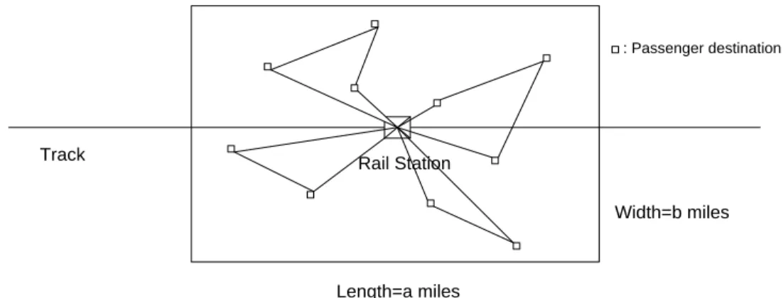
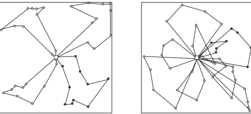
Figure 2.10 Best routes for a 𝒋 = 𝟒𝟎, 𝒄 = 𝟏𝟎 instance (left), a 𝒋 = 𝟒𝟎, 𝒄 = 𝟒 instance (right)
To assess the accuracy of (2.18), we took advantage of the fact that good heuristics exist for the VRP. Specifically, we simulated hundreds of thousands of instances of LMTS train arrivals and associated customer destinations. To create the clusters and routes we applied two widely used VRP heuristics, the Sweep algorithm (coupled with a TSP heuristic) and the Clark-Wright algorithm. According to Cordeau et al. (2002), these fast and simple heuristics provided an average deviation of 6.71% and 7.09%, respectively, from the best solutions obtained on CMT benchmark instances. We solved all the simulated instances we generated using each of the two heuristics separately and, for each instance, we chose the better of the two solutions. Figures 2.10 shows the best solutions obtained for two examples, both with 𝑗 = 40 customers but in one case with 𝑐 = 10 and in the other with 𝑐 = 4. As might be expected, the Sweep algorithm generated the solution shown on the left and Clark-Wright the one shown on the right. For a broad range of vehicle capacities, 𝑐 (2 to 20), and number of routes 𝑗/𝑐 (2 to 20), the average error of (18), in absolute value terms, was of the order of 2%. Table 2.1 shows part of this assessment.