Design and Optimization of Complex Systems

1

Design and Optimization of Complex Systems

Karen Willcox

Abstract

Truely optimal solutions to system design can only be obtained if the entire system is considered. In this research we consider design of commercial aircraft, but we expand the system to include a family of planes. A multidisciplinary design optimization framework is developed in which multiple aircraft, each with different missions, can be optimized simultaneously. Results are presented for a two-member family whose individual missions differ significantly. We show that both missions can be satisfied with common designs, and that by optimizing both planes simultaneously rather than following the traditional baseline plus derivative approach, the common solution is vastly improved. The new framework is also used to gain insight to the effect of design variable scaling on the optimization algorithm.

Introduction

In today’s competitive environment, the aerospace industry is faced with the challenge of designing aircraft not only with superior performance, but also at a lower cost. Multidisciplinary design optimization (MDO) is a tool that has been used successfully throughout the design process to enable improvements in aircraft performance. By simultaneously considering the effects of aerodynamics, structures, propulsion, flight mechanics and dynamics, and the complicated interaction between them, substantially improved performance can be achieved.

Studies show that the aircraft industry has evolved to a “dominant design”, and that factors such as cost are becoming increasingly important [1]. In the “Better, Faster, Cheaper” era, the aerospace industry is searching for ways to lower costs without compromising aircraft performance.

One way to reduce costs is to conceive of a family of aircraft who share common characteristics, such as planform and systems, but who each satisfy a different mission requirement. Traditionally this has been achieved through the use of derivatives. A baseline aircraft is designed and subsequently modified to produce a number of derivatives to satisfy different missions (e.g. longer range, carry more payload). By taking advantage of commonality with the existing base model, it is possible to achieve the new mission at a far lower cost than would be incurred if a completely new

plane were designed. Often, the modifications can be substantial, resulting in an almost entirely new plane. For example, the Boeing 737 Next Generation has a completely new wing.

Here, the concept of commonality is taken a step further. We consider not just commonality between derivative aircraft whose missions are similar, but between two planes whose missions differ significantly. For example, if one could design a small capacity and a large capacity aircraft with common characteristics (for example a common wing), substantial savings could be realized in both recurring cost (manufacturing) and non-recurring cost (design effort and tooling cost). The savings from commonality come at a price: the weight of these common planes will be higher than if each were optimized separately for its own mission. The question then, is whether it is possible to design a family of common planes that satisfies all missions but whose cost saving outweighs the weight penalty. An example of this exists in practice: the Airbus A330 and A340 planes share common wings.

Fujita et al. [2] discuss the simultaneous optimization of a family of products, however they assume that a baseline has been designed, and then consider the design of derivatives from this baseline. The mission of these derivatives is fairly close to the original: in the example they present, the only change to the derivative mission is to extend the range. In all cases, the derivative carries the same payload and retains the original fuselage.

In this research, a common family is designed from a more fundamental approach. Optimization of a system which encompasses multiple aircraft is performed. As an example, we consider the Blended-Wing-Body (BWB), a revolutionary concept for transport that integrates wing, fuselage, engines, and tail to achieve a

2 substantial improvement in performance over a conventional transport (Figure 1 and References [3,4]). Here, the specifics of the MDO approach are described and the simultaneous optimization and commonality framework are outlined. An example is presented in which a family of two BWB aircraft are designed. One plane will be large and long-range (475 passengers, 8550 nm), while the second will be smaller and long-range (272 passengers, 8550 nm). Finally, we present some conclusions and directions of ongoing and future work.

Multidisciplinary Design Optimization Framework

As described in [5] and [6], WingMOD is an MDO code that optimizes aircraft wings and horizontal tails subject to a wide array of practical constraints. WingMOD was initially applied to the design of a composite wing for a stretched MD-90 [7] and then went through considerable modification for application to the BWB [8,9]. The BWB planform is modeled as a series of spanwise elements as shown in Figure 2. Optimization services for WingMOD are provided by the Genie framework [8].

WingMOD uses intermediate fidelity analyses to quickly analyze an aircraft in over twenty design conditions that are needed to address issues from performance, aerodynamics, loads, weights, balance, stability and control. The low computational cost of the intermediate fidelity analyses allows the examination of all these issues in an optimization with over a hundred design variables while achieving reasonable computation time.

The basic WingMOD method models an aircraft wing and tail with a simple vortex-lattice code and monocoque beam analysis, coupled to give static aeroelastic loads. The model is trimmed at several flight conditions to obtain load and induced drag data. Profile and compressibility drag are evaluated at stations across the span of the wing with empirical relations using the lift coefficients obtained from the vortex lattice code. Structural weight is calculated from the maximum elastic loads encountered through a range of flight conditions, including maneuver, vertical gust, and lateral gust. The structure is sized based on bending strength and buckling stability considerations. Maximum lift is evaluated using a critical section method that declares the wing to be at its maximum useable lift when any section reaches its maximum lift coefficient, which is calculated from empirical data. Balance is evaluated by distributing weight over the planform as described in [10].

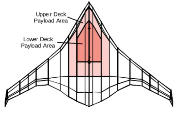
Uppe r Deck Payload Area Lower Deck Payload Area

Figure 2: WingMOD BWB Model.

The optimization algorithm used is sequential quadratic programming (SQP). The nonlinear problem can be stated as

minimize

F

( x

)

subject to

c

(

x

)

≥

0

,

i

=

1

,

2

,

K

,

m

functions. The Hessian matrix of F(x) contains the second order variations of the objective function with respect to each design variable, and is given by the

n x n matrix G(x):





























∂

∂

∂

∂

∂

∂

∂

∂

∂

∂

≡

≡

∇

)

(

)

(

x

F

x

x

F

x

x

F

x

F

x

G

x

F

L

M

M

L

The SQP algorithm uses a sequence of line searches to determine the optimum solution to the nonlinear problem (1). The design space is modeled as a quadratic objective with linear constraints, using finite difference gradient calculations. An approximate Hessian matrix is constructed from information gathered over the sequence of iterations using the Broyden-Fletcher-Goldfarb-Shanno (BFGS) update [11]. A quadratic programming problem is solved in the approximate design space to determine an estimated best direction for improvement. A line search is then executed in the actual design space which seeks improvement in the solution.

Convergence of the algorithm is critically dependent, amongst other things, on the conditioning of the Hessian matrix. In [11] an approximate estimate is derived for the accuracy of the solution. Given the computed optimal solution

x

x

*

3

p

x

G

p

x

x

*)

(

2

*

≈

ε

−

where

ε

perturbation vector of unit length. Equation (3) shows that if G(x*) is ill-conditioned, then the error in the computed solution can be very large along certain directions. As stated in [11], since the objective function will vary much more rapidly in some directions than in others, an ill-conditioned Hessian is a form of bad scaling. This scaling problem may also have an adverse effect on the optimization algorithm itself, since the objective may vary extremely slowly along directions associated with a small eigenvalue. In this case, changes in the objective that are significant may be lost, and the algorithm will have trouble converging to the exact solution.

The ill-conditioning of the Hessian matrix can be quantified by its condition number given by

1

)

(

)

(

)

(

≥

=

G

G

G

λ

λ

κ

where λmax(G) and λmin(G) are respectively the

maximum and minimum eigenvalues of G. (Note that because G is a symmetric matrix its eigenvalues and singular values are the same.) A matrix is said to be well-conditioned if its condition number is small (~1), and ill-conditioned if

κ

We can therefore ensure that (1) is a well-scaled problem by choosing a linear transformation of the design variables that minimizes the condition number of the Hessian matrix at the solution. In practice this is done a posteriori: once the algorithm has converged to the calculated optimum, the Hessian matrix is inspected. Experience has shown that the approach can be simplified: by considering only the diagonal elements of

)

( x

G

Simultaneous Optimization with Commonality

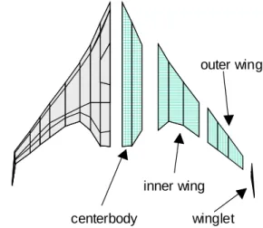
The MDO framework described in the previous section was altered to allow the simultaneous optimization of multiple planes with varying levels of commonality. Constraints arising from each of the disciplines were generated for each plane in the family. Commonality between family members was defined by breaking each plane into components. There were four main structural components: centerbody, inner wing, outer wing and winglet as shown in Figure 3. Each of these components can be specified to be either common or uncommon between family members. If just a particular component is allowed to vary, then the interface with a neighboring

common component is kept common. An example might be allowing the centerbody to vary between family members, but keeping a common wing. In this case, the interface between the centerbody and the wing will be kept common.

centerbody

inner wing

outer wing

winglet Figure 3: Modular structural breakdown of BWB.

Since making parts common is a discrete decision, the effect of varying levels of commonality is assessed via trade studies rather than being determined through the optimizer. In the problem setup, parts can be made common by either enforcing explicit constraints on their dimensions or linking the dimensions so they always have the same value. The ability to link variables was added to the Genie framework that supports WingMOD. When a chord at a spanwise location on Plane 1 is linked to the corresponding chord on Plane 2, Genie causes changes on either chord to be immediately reflected on the other. The optimizer then views each set of linked variables as a single quantity. This approach is more efficient than having a design variable for each chord and an explicit commonality constraint to force the variables to be equal: it eliminates a design variable and constraint for each linked variable thus reducing the overall size of the combined optimization problem.

Fujita et al. [2] state that when the difference between product characteristics is large, two independent products must be designed, since “commonalization of parts cannot meet with performance requirement, even though it is effective for cutting cost”. They do not attempt to quantify a “large difference”, although the examples they discuss (stretching a baseline design to extend range/payload) suggest that the missions of each family member are only incrementally different. Using the methodology developed here, a solution can be determined that does satisfy all performance requirements, even when the product characteristics are

4 significantly diverse. Subsequently, a cost analysis can be applied to determine whether such a design is a viable option.

One approach to designing a common family might be to first optimize one family member and then force subsequent family members to share appropriate common features with the established planform. For example, in designing a small and a large plane with common planforms, one could first optimize the large plane, and then construct a smaller plane from the resulting planform. There are two problems with this approach. First, as pointed out in [2], there is no guarantee that the solution obtained from the first optimization will satisfy all constraints on other family members. In the two-plane example, it is likely, although not certain, that the planform arising from optimizing a large plane will satisfy all requirements on the smaller plane. This may not be the case if we were to add a third family member. The second issue is that this sequential approach results in a sub-optimal family. For example, by trading some optimality on the larger plane, significant improvement could be obtained in the smaller plane, resulting in an overall “better” family solution. This raises the issue of what the objective should be in the family optimization: should we try to minimize the combined weight of the family, or should the objective be more heavily biased towards a certain family member? The results presented in the following section will demonstrate that simultaneous optimization overcomes the limitations of sequential optimization of a family. A discussion of the choice of appropriate objectives will also follow.

Results and Discussion

Results will be presented for design of a two-member BWB family. The two planes satisfy the following mission requirements:

Plane 1: 8550 nm range, 475 passengers Plane 2: 8550 nm range, 272 passengers These two planes represent what might be the smallest and largest aircraft of a family with more members, i.e. this would be the greatest mission difference of interest.

Example 1: Simultaneous Point Optimization of Two Planes

In order to investigate the new multiple-aircraft optimization framework, a test problem was set up. The two planes were designed simultaneously, but with no commonality constraints. Obviously, the solution to this problem could be obtained by optimizing each plane separately. Since the actual solution of the problem can be determined using the conventional approach, valuable insight to the new framework can be gained. This example highlights the importance of design variable scaling discussed in Section 2. Initially the simultaneous design problem was set up by simply concatenating the constraints for each plane, and attempting to minimize the sum of the take-off weights. Each problem was also optimized individually to determine the minimum-weight solution for each plane. In each individual case, the optimizer converged without difficulty. Despite identical systems being used in the simultaneous setting with no coupling between them, the optimizer could not converge to the correct optimal solution. The minimum-weight solution was obtained for Plane 1 (the larger plane), however the solution for Plane 2 was significantly sub-optimal when the algorithm claimed to have converged. Inspection of the Hessian matrix at this solution showed that geometric variables associated to Plane 2 were badly scaled. The diagonal entries of the Hessian for these variables were O(10-2) and O(10-3).

The troublesome variables were rescaled, and the simultaneous optimization was performed again. Now the optimizer had no trouble converging to a solution that agreed with the individually obtained optimal designs. The calculated weights for the final 100 iterations are plotted in Figure 4. Shown are the calculated take-off weights for each plane, normalized by the known point-optimum solution. The results are very similar for Plane 1 in both the scaled and unscaled cases. In the unscaled case, the solution has converged to a sub-optimum level for Plane 2.

This result suggests that in the simultaneous framework, the optimization algorithm is much more sensitive to poor scaling. This can be explained mathematically by comparing the Hessian matrices of the individual and 0.99 1 1.01 1.02 1.03 0 20 40 60 80 100 Iteration number M T OW ( n or m a li z e d) Plane 1 Plane 2 (scaled) Plane 2 (unscaled)

Figure 4: Objective history for optimization algorithm. Shown are the calculated weights for each plane over the last 100 iterations, normalized

5 combined systems. If the Hessian of the system for Plane 1 alone is G1 and for Plane 2 is G2, then the

Hessian of the simultaneous system is given by













=

0

0

G

G

G

since there is no coupling between the planes. The condition numbers of the single-plane Hessians are

( )

λ

λ

κ

G

=

( )

λ

λ

κ

G

=

and for the combined system:

( )

(

₍

₎

)

,

min

,

max

λ

λ

λ

λ

κ

G

=

From equation (7) we can see that in the best case the condition number of the combined system will be equal to the worst of

κ

(

G

)

κ

(

G

)

exceed both.

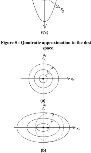
One can gain an understanding of how poor scaling might affect the convergence of the optimization algorithm by considering a simple geometric representation of the problem. Consider a system with two design variables. In the SQP algorithm, at each step the design space is modeled as a quadratic objective with linear constraints. If we were to plot the objective versus each of the design variables, we would obtain a paraboloid as shown in Figure 5. If the design variables are perfectly scaled so that the Hessian matrix has a condition number of unity, then the cross-sectional slices of the paraboloid are circles. If one (or both) of the variables is badly scaled, then the cross sections of the paraboloid are elliptical. In fact, the relative lengths of the major and minor axes of the ellipse are described by the minimum and maximum eigenvalues of the Hessian matrix.

Figure 6 demonstrates how the algorithm might be adversely affected by poor scaling. In both diagrams, the optimum is located at the origin. In the well-scaled case (a), the objective contours are circles and the line search moves the solution in the correct direction. Now consider the case in Figure 6(b) where variable x1 is

well scaled, but x2 is badly scaled. The line search will

choose a direction that captures the correct behavior for

x1, but very little improvement in x2. If the scaling

problem is bad enough, the optimizer will converge to a sub-optimal solution represented by the star in Figure 6(b) where the remaining improvement in x2 cannot be

achieved. Figure 6(b) describes the BWB example very closely. One could consider x1 as representing all design

variables for Plane 1 and x2 as representing all those for

Plane 2. Because x2 was poorly scaled, the optimizer

achieved the true minimum-weight solution for Plane 1, but converged to a sub-optimal solution for Plane 2.

Example 2: Optimizing a Two-Plane Common Family

We now present results for the two-plane family with commonality. The planes are constrained to have completely common wings (inner wing, outer wing and winglet in Figure 3), but different centerbodies. The interface between the inner wing and the centerbody is also common. The results will be used to assess the value of the new, simultaneous design approach.

The two-plane family was first designed using a conventional, sequential technique. The larger plane was optimized for minimum take-off weight as if it were a point design. The smaller plane was then optimized to achieve its minimum take-off weight, but constrained to have an identical wing to its pre-determined larger

F(x)

x

1

x

2

Figure 5 : Quadratic approximation to the design space. (a) (b) x x x 1 x 2 x 1 x 2

Figure 6: Geometric interpretation of QP line search. Well scaled (a) and badly scaled (b) cases.

6 mate. This resulted in what we refer to as the sequential

family design. The new optimization framework was

used to design the two planes simultaneously by minimizing the sum of the take-off weights, resulting in the simultaneous family design. Table 1 summarizes the results for the simultaneous optimization. The total take-off weight for the simultaneous family is 3395 lb less than that of the sequential family. This weight reduction is achieved by a small increase in the weight of Plane 1, which allows a significant decrease in the weight of Plane 2, resulting in an overall better solution.

Table 1: Optimization results for simultaneous family design. Changes are relative to the sequential

design solution. Total MTOW MTOW Plane 1 MTOW Plane 2 -3395 lb +573 lb -3968 lb

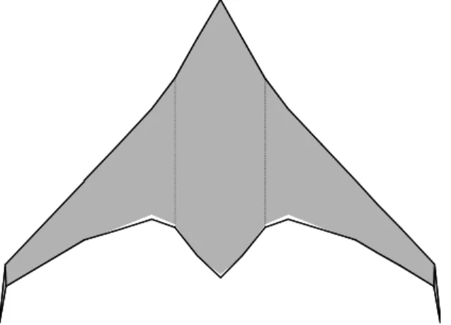
Further interrogation of the solutions shows how the optimizer has made trade-offs to achieve this weight reduction. The wing area (and hence structural weight) of Plane 1 has been slightly reduced at the expense of aerodynamic efficiency. A decrease in structural weight of 0.45% is traded for a reduction in average cruise lift to drag ratio of 0.35%. Although this means that the take-off weight for Plane 1 is slightly greater than the point-optimum solution, the reduced wing area has very positive benefits for Plane 2. In the sequential design, the constrained wing area for Plane 2 is significantly larger than is actually required. Reduction of the area lowers the structural weight without compromising aerodynamic efficiency, which means that a further cut in weight is achieved via a lowered fuel requirement.

Figure 7 depicts the two different planforms for Plane 2. The comparison shows how the diminished wing area has been achieved: reduced chords and slightly increased sweep.

Choice of Objective

When designing more than one plane, the objective should be chosen by careful consideration of the problem at hand. As mentioned previously, commonality between family members results in a trade-off between increased operating cost (weight) and reduced acquisition cost (manufacturing/development). Ultimately, we plan to incorporate a cost model to the MDO framework and to optimize the family by maximizing profit rather than by minimizing weight. Development of a suitable cost modeling framework is underway. In this expanded framework, the appropriate objective will be clear: maximize the overall profit associated to the family. In the current model where we consider take-off weight, it is necessary to choose an appropriate objective that includes a weighted contribution from each family member. For a family with Nf members, the objective takes the form

min













∑

W

s

where 0<si<1 is a weighting factor for the ith plane and

Wi is its take-off weight. In many cases, simply

minimizing the sum of the family take-off weights will be a suitable approach (si=1/Nf, i =1...Nf). If other

factors are taken into consideration, such as relative market demands or competing aircraft, then an objective should be chosen which favors the most critical family members.

Investigation into the effect of objective choice was performed for the two-plane common-wing family. Three optimizations were carried out with varying weighting factors, si, on the take-off weights of each

plane. The results are summarized in Table 2.

Table 2: Optimization results for different objectives. Changes are relative to the sequential

design solution. s1 s2 MTOW Plane 1 MTOW Plane 2 Total MTOW 0.5 0.5 +584 lb -1545 lb -961 lb 0.1 0.9 +1800 lb -2282 lb -482 lb 0.9 0.1 +298 lb -405 lb -107 lb

While the first optimization provides the lowest total take-off weight, the weight of the smaller plane can be further reduced by biasing the objective function in its

Figure 7: Planforms for Plane 2: wings common with Plane 1, centerbody optimized. Sequential (black line) and simultaneous (grey shade) designs.

7 favor. Again, a reduction of the aerodynamic efficiency of the large plane is traded for reduced wing area. With a large weighting placed on Plane 1, the simultaneous design begins to approach its point-optimal solution. Within the simultaneous optimization framework, the objective choice can be used to rigorously balance the compromise between family members. It would be extremely difficult to identify these trade-offs when working with a sequential design method.

Conclusions

Simultaneous optimization of multiple aircraft offers considerable benefit to the design process. By designing family members with common characteristics, substantial savings can be realized in manufacturing and development costs. The simultaneous optimization methodology presented here not only ensures that a common design can be found which satisfies all constraints on each family member, but also determines the best overall family solution by applying appropriate trade-offs between aircraft. The results presented demonstrate that a common solution can be found even when mission requirements differ significantly between family members. Substantial weight savings can be achieved by designing family members simultaneously and allowing the optimizer to make apt trade-offs. The next stage in this work is to develop a cost model that can capture the benefits of commonality. Preliminary cost analysis indicates that the weight penalties incurred by the common design are more than offset by savings in manufacturing and development cost. A detailed cost modeling framework is currently under development, which will allow the benefits of common design to be assessed more accurately.

References

1 Murman, E.M., Walton, M. and Rebentisch, E., “Challenges in the Better, Faster, Cheaper Era of Aeronautical Design, Engineering and Manufacturing”,

The Aeronautical Journal, October 2000, pp 481-89.

2 Fujita, K., Akagi, S., Yoneda, T. and Ishikawa, M., “Simultaneous Optimization of Product Family Sharing System Structure and Configuration”, Proceedings of ASME Design Engineering Technical Conference, September 1998, Atlanta, GA.

3 Liebeck, R. H., Page, M. A., Rawdon, B. K., “Blended-Wing-Body Subsonic Commercial Transport,” AIAA Paper 98-0438, Jan. 1998.

4 “Blended-Wing-Body Technology Study,” Final Report, NASA Contract NAS1-20275, Boeing Report CRAD-9405-TR-3780, Oct. 1997.

5 Wakayama, S., Kroo, I., “Subsonic Wing Planform Design Using Multidisciplinary Optimization,” Journal

of Aircraft, Vol. 32, No. 4, Jul.-Aug. 1995, pp.746-753.

6 Wakayama, S., Lifting Surface Design Using

Multidisciplinary Optimization, Ph.D. Thesis, Stanford

University, Dec. 1994.

7 Wakayama, S., Page, M., Liebeck, R., “Multidisciplinary Optimization on an Advanced Composite Wing”, AIAA Paper 96-4003, Sep. 1996. 8 Wakayama, S., Kroo, I., “The Challenge and Promise of Blended-Wing-Body Optimization”, AIAA Paper 98-4736, Sep. 1998.

9 Wakayama, S., “Multidisciplinary Optimization of the Blended-Wing-Body”, AIAA Paper 98-4938, Sep. 1998.

10 Wakayama, S., “Blended-Wing-Body Optimization Problem Setup”, AIAA Paper 2000-4740, Sep 2000. 11 Gill, P.E, Murray, W. and Wright, M.H., Practical