Knowledge management for collaborative design and multi-physical optimization of mechatronic systems

(1)

HAL Id: tel-02463955

https://tel.archives-ouvertes.fr/tel-02463955

Submitted on 2 Feb 2020

Knowledge management for collaborative design and

multi-physical optimization of mechatronic systems

Mehdi Mcharek

To cite this version:

Mehdi Mcharek. Knowledge management for collaborative design and multi-physical optimization of mechatronic systems. Mechanical engineering [physics.class-ph]. Université Paris Saclay (COmUE), 2018. English. �NNT : 2018SACLC098�. �tel-02463955�

(2)

Gestion des connaissances pour la

conception collaborative et

l’optimisation multi-physique de

systèmes mécatroniques

Thèse de doctorat de l'Université Paris-Saclay Préparée à CentraleSupélec École doctorale n°573 approches interdisciplinaires, fondements, applications et innovation (Interfaces) Spécialité de doctorat: Sciences et technologies industrielles

Thèse présentée et soutenue à Saint Ouen, le 12/12/2018, par

Mehdi Mcharek

Composition du Jury :

Jean Bigeon

Directeur de recherche à l’INP Grenoble Président Marc Budinger

Maître de conférences HDR à l’INSA Toulouse Rapporteur Nadine Piat

Professeur à l’ENSMM Besançon Rapporteuse

Jean-Marc Faure

Professeur à Supméca Paris Examinateur

Stanislao Patalano

Associate professor à l’unviversité Frederico II Naples Examinateur Jean-Yves Choley

Profeseur à Supméca Paris Directeur de thèse Cherif Larouci

Maître de conférences HDR à l’Estaca Co-directeur de thèse Moncef Hammadi

Maître de conférences à Supméca Paris Invité Toufik Azib

Maître de conférences à l’Estaca Invité

N N T : 20 18 S A C LC 09 8

(3)

Title: Knowledge management for collaborative design and multi-physical optimization of

mechatronic systems

Keywords: Knowledge Management (KM), Collaborative design, Design process,

Multidisciplinary Design Optimization (MDO), Mechatronic systems, Electronic Throttle Body

Abstract: Mechatronic products are complex

and multidisciplinary in nature. The requirements to design them are often contradictory and must be validated by the various disciplinary engineering (DE) teams. To address this complexity and reduce design time, disciplinary engineers need to collaborate dynamically, resolve interdisciplinary conflicts, and reuse knowledge from previous projects. In addition, they need to work seamlessly with the Systems Engineering (SE) team to have direct access to requirements and the Multidisciplinary

We propose to use Knowledge Management techniques to structure the knowledge generated during collaboration activities and harmonize the overall design cycle. Our primary contribution is a unification approach, elaborating how SE, DE, and MDO complement each-other and can be used in synergy for an integrated and continuous design cycle. Our methodology centralizes the product knowledge necessary for collaboration. It ensures traceability of the exchange between disciplinary en-gineers using graph theory. This

Titre: Gestion des connaissances pour la conception collaborative et l’optimisation multi-physique

de systèmes mécatroniques

Mots clés: Gestion des connaissances, conception collaborative, processus de conception,

optimisation multidisciplinaire, systèmes mécatroniques, boitier papillon

Résumé: Les produits mécatroniques sont

complexes et multidisciplinaires par nature. Les exigences pour les concevoir sont souvent contradictoires et doivent être validées par les différentes équipes d'ingénierie disciplinaire (ID). Pour répondre à cette complexité et réduire le temps de conception, les ingénieurs disciplinaires ont besoin de collaborer dynamiquement, de résoudre les conflits interdisciplinaires et de réutiliser les connaissances de projets antérieurs. De plus, ils ont besoin de collaborer en permanence avec l’équipe d’ingénierie systèmes (IS) pour avoir un accès direct aux exigences et l’équipe d’optimisation multidisciplinaire (OMD) pour valider le système dans sa globalité.

Nous proposons d'utiliser des techniques de gestion des connaissances pour structurer les connaissances générées lors des activités de collaboration afin d'harmoniser le cycle de conception. Notre principale contribution est une approche d'unification qui explique comment IS, ID et OMD se complètent et peuvent être utilisés en synergie pour un cycle de conception intégré et continu. Notre méthodologie permet de centraliser les connaissances nécessaires à la collabora-tion et au suivi des exigences. Elle assure également la traçabilité des échanges entre les ingénieurs grâce à la théorie des graphes. Cette connaissance formalisée du processus de collaboration permet de défi-nir automatiquement un problème OMD.

(4)

(5)

Acknowledgements

I dedicate this work to my parents for their unconditional love and support.

I would like to thank my supervisors Moncef Hammadi and Toufik Azib. You always were present for me and this work could not exist without your contributions. I really enjoyed work-ing with you and sharwork-ing with you these nice three years!

I address my thanks to my directors Jean-Yves Choley and Cherif Larouci for welcoming me and providing me the appropriate conditions. You have always encouraged and guided me throughout this adventure, thank you!

I would like to thank Nadine Piat and Marc Budinger for accepting to review my PhD manu-script, for the quality of their reports, and their interesting questions. I address my thanks to Jean Bigeon for presiding the defense, as well as Stanislao Patalano and Jean-Marc Faure to examine this thesis. I appreciated your comments and valuable advice. Special thanks to Su-zanne Thuron for the organization.

I express my gratitude to the members of the MIMe project, for their motivation and the con-structive meetings that have enriched my work. Special thanks to Simon Midrier, Antoine Na-varro, Abdoulaye Sow, Antoine Munck, Matthieu Bricogne, Kevin Maquin, Harvey Rowson, Françoise Caron, and Joseph Aracic. It was really a pleasure to collaborate with you. The ex-perimental validations, industrial requirements, beta-testing, interviews were crucial in this work and all the members have made their best to achieve these goals, thank you!

I am grateful to the members of Quartz Laboratory for all the moments that we shared together. Thanks to Christelle, Amel, Régis, Reda, Olivia, and Faida for your support, availability and kindness. I would like to thank Lionel who've left us this year and who delighted us with his smile, enthusiasm and helpfulness. I am also grateful to the members of Estaca’Lab for wel-coming me and for the stimulating discussions. Thanks to Sandrine, Georges, Amine, Adriano,

(6)

(7)

Figure 0-1. MIMe project organization ... 23 Figure 0-2. Organization of the manuscript chapters ... 25 Figure 1-1. Mechatronic applications (Karnopp, Margolis et al. 2012) ... 30 Figure 1-2. Mechatronic system architecture (adapted from (Krause, Jansen et al. 2007)) ... 31 Figure 1-3. Examples for mechatronic components (Hehenberger and Zeman 2007) ... 32 Figure 1-4. Electronic throttle body environment (Nentwig and Mercorelli 2008) ... 33 Figure 1-5. Electronic Throttle Body composition ... 33 Figure 1-6. Mechatronic sequential process (Shetty, Manzione et al. 2012)35 Figure 1-7. Design cycle of mechatronic systems (adapted from VDI Guideline) ... 37 Figure 1-8. SE, DE, and MDO activities in mechatronic design ... 38 Figure 1-9. Diagrams of SysML language (Friedenthal, Moore et al. 2014)40 Figure 1-10. Black box-white box approach (Mhenni, Choley et al. 2014) 40 Figure 1-11. Integration modeling approach (Abid, Pernelle et al. 2015) ... 41 Figure 1-12. Functional architecture of the ETB (Ammar, Hammadi et al. 2017) ... 41 Figure 1-13. Two architectures of the ETB ... 42

(14)

Figure 1-18. Modelica model of ETB in open loop ... 48

Figure 1-19. System response with 90° as an initial position to illustrate springs effects ... 49

Figure 1-20. The All At Once problem formulation (Lambe and Martins 2012) 51 Figure 1-21. XDSM of a multidisciplinary analysis (MDA) process to solve a three-discipline coupled system ... 52

Figure 1-22. Examples of PIDO frameworks ... 54

Figure 1-23. Pareto front in multi-objective optimization ... 54

Figure 1-24. Robust vs local vs global optimum ... 55

Figure 1-25. The three steps of the surrogate modelling process ... 56

Figure 1-26. Space mapping principle ... 56

Figure 1-27. Modelica model for optimization ... 58

Figure 1-28. Optimization between modelica and ModelCenter software .. 58

Figure 1-29. Pareto Front solution ... 59

Figure 1-30. Comparison between the initial and the optimized set ... 60

Figure 1-31. Research problematic ... 63

Figure 2-1. PLM functions in the entire product process (Matta, Ducellier et al. 2013) ... 66

Figure 2-2. Design knowledge and freedom related to the design cycle (Verhagen, Bermell-Garcia et al. 2012) ... 67

Figure 2-3. Spiral conversion of knowledge (Nonaka 1991) ... 68

Figure 2-4. Classifying knowledge in three axes (Chandrasegaran, Ramani et al. 2013) ... 70

Figure 2-5. Knowledge representations throughout the product lifecycle (Ali 2016) ... 71

Figure 2-6. Overview of KM, KE and KBE (Chandrasegaran, Ramani et al. 2013) ... 73

Figure 2-7. MOKA methodology process (MOKA Group, 2000) ... 74

(15)

Figure 2-9. Conceptual architecture of SLIM (Bajaj, Zwemer et al. 2011) 78 Figure 2-10. SysML-PIDO connection using MagicDraw and ModelCenter

software (Kaslow, Soremekun et al. 2014) ... 79

Figure 2-11. Multiviewpoint concept (Törngren, Qamar et al. 2014) ... 80

Figure 2-12. PROXIMA framework ... 81

Figure 2-13. Knowledge Management Model ... 82

Figure 2-14. COLIBRI concept (Kleiner, Anderl et al. 2003) ... 83

Figure 2-15. Design and Engineering Engine process (La Rocca 2012) ... 85

Figure 2-16. FabK Methodology (Toussaint, Demoly et al. 2010) ... 86

Figure 2-17. KADMOS methodology overview (van Gent, Ciampa et al. 2017) 87 Figure 3-1 Knowledge Configuration Model principle ... 91

Figure 3-2 UML meta-model of KCM (Monticolo, Badin et al. 2015) ... 94

Figure 3-3. KCM-PLM connection (Penciuc, Durupt et al. 2014) ... 95

Figure 3-4. SE-DE connection using KCM ... 97

Figure 3-5. MDO - KCM connection ... 99

Figure 3-6. Siemens VDO model ... 100

Figure 3-7. ETB architecture in closed loop ... 101

Figure 3-8. Modelica model of the ETB in closed loop ... 101

Figure 3-9. Hysteresis behavior of the ETB ... 102

Figure 3-10. KARREN platform dashboard ... 104

Figure 3-11. Karren - Isight connection ... 104

Figure 3-12. Sequential diagram of the collaboration ... 105

(16)

Figure 4-4. System and interdisciplinary conflicts management in CDPPK118

Figure 4-5. Exchange graph between DE models ... 120

Figure 4-6. KADMOS platform overview (van Gent, Ciampa et al. 2017)122 Figure 4-7. Design Product Knowledge in Python demonstrator ... 123

Figure 4-8. Collaborative Design Process in the Python demonstrator ... 124

Figure 4-9. Graph generation in Python ... 125

Figure 4-10. Connection between design product and process knowledge 126 Figure 4-11. Knowledge management in CDPPK ... 127

Figure 5-1. Multi-physical model of the ETB using Modelica ... 129

Figure 5-2. Control model of the ETB using Simulink software ... 130

Figure 5-3. Fluid model of the ETB using Ansys ... 131

Figure 5-4. Experimental test bench of the ETB ... 132

Figure 5-5. ICEs definition in DPK ... 134

Figure 5-6. UPCs involved in the collaboration ... 136

Figure 5-7. The different users involved in the collaborative scenario ... 137

Figure 5-8.Collaboration graph generated by Python demonstrator ... 138

Figure 5-9. The system response to the complete profile reference ... 139

Figure 5-10. 3D model to estimate the airflow section of the ETB ... 141

Figure 5-11. Collaborative process generated by CDPPK ... 142

Figure 5-12. XDSM of the IDF architecture applied to the ETB problem 143 Figure 5-13. Automatic MDO problem generation in RCE environment . 144 Figure 5-14. Airflow section estimation ... 145

Figure 5-15. Discharge coefficient for each throttle angle ... 145

Figure 5-16. Optimized mass flow model ... 146

Figure 5-17. Rising time, return time and the maximum current of the ETB147 Figure 5-18. Step function response of ETB ... 147

(17)

(18)

(19)

List of Tables

Table 1-1. Example of stakeholders and their roles in the automotive domain (Navet

and Simonot-Lion 2008) ... 45

Table 1-2. ETB initial parameters ... 48

Table 1-3. Optimization problem ... 57

Table 1-4. Four selected solutions ... 59

Table 2-1. Criteria for KM mechatronic platform ... 75

Table 2-2. SysDICE framework evaluation ... 77

Table 2-3. SLIM framework evaluation ... 78

Table 2-4. SysML-PIDO framework evaluation ... 79

Table 2-5. Multiviewpoint framework evaluation ... 80

Table 2-6. PROXIMA framework evaluation ... 81

Table 2-7. KCM framework evaluation ... 82

Table 2-8. COLIBRI framework evaluation ... 84

Table 2-9. DEE framework evaluation ... 85

Table 2-10. FabK framework evaluation ... 86

Table 2-11. KADMOS framework evaluation ... 87

Table 2-12. Summary of frameworks evaluation ... 87

Table 3-1. List of parameters and ICEs ... 102

Table 5-1. The list of crucial parameters and the values found by users ... 134

(20)

Introduction

A. General introduction

Recent advances in design methods promote the development of concurrent engineering to reduce the time and cost of the design cycle. This is particularly necessary for mechatronic design which is involving several disciplines. But companies have also to address associated challenges related to collaboration and reuse. For instance, designers from different disciplines need to collaborate instan-taneously and access to the right information at the right moment (Maranzana, Gartiser et al. 2008). Mechatronic systems encompass a variety of disciplines, including control, electrical and software. They need to be combined to accomplish the entire requisite functionality (Zheng, Bricogne et al. 2014). Each discipline independently focuses on a particular aspect of the system and exploits differ-ent Disciplinary Engineering (DE) tools for technical analysis. Such multiplicity of tools and methods renders the mechatronic design quite complex and knowledge intensive. Systems Engineering (SE) approach was proposed to manage this issue. It provides a common communication platform between different stakeholders at the system level, ensuring that each discipline meets the system require-ments. Despite these efforts, a benchmark report about mechatronic design challenges shows that 44% of the manufacturers have a problem with understanding and fulfilling requirements (Jackson 2006). To attain the full benefit of SE in concurrent engineering, there is a critical need to create links between system engineers and disciplinary engineers. Research reports a gap between SE and DE, resulting in costly failures to meet system requirements (Gausemeier, Gaukstern et al. 2013). Solu-tions must support the collaboration between the two levels, allowing system engineers to manage changes in requirements and access dynamic decisions, made during the design cycle, and discipli-nary engineers to solve their conflicting objectives and to stay consistent with the system level. Mul-tidisciplinary Design Optimization (MDO) was proposed as a solution to this issue. It provides useful instruments and methodologies to deal with complex design problems. Nevertheless, MDO is chal-lenging to implement in an industrial environment and cannot handle for itself the complexity of the dynamic collaboration and complex reuse of project results (Simpson, Toropov et al. 2008).

In our manuscript, we will study the links between SE, DE and MDO and how to merge them for an integrated and continuous mechatronic design cycle.

B. Research context

(21)

This thesis is a part of a collaborative French project entitled FUI19-MIMe (Model d’Intégraton et de Simulation Mécatronique), which brings together industrials and academics:

- Small and medium-sized enterprises: DPS, Deltacad, Soyatec, and Eiris - Manufacturers: PSA and Valeo

- Academics: Supmeca, Estaca, and UTC

The MIMe project aims to enable structured and instantaneous collaboration in mechatronic design. PSA and Valeo are two major French automotive manufactures. Many meetings were conducted in the context of this project to identify the industrial requirements and the problems relative to mecha-tronic design. While each work package of the MIMe project focuses on specific objectives, the meet-ings were valuable to exchange our views and converge in our research.

b. Project objectives

The MIMe project is divided into 5 work packages. Our Ph.D. thesis is situated in the WP4. The different WPs meet regularly to keep the coherence of the global project.

(22)

WP2: UTC - DeltaCAD

Determines how to capitalize multidisciplinary knowledge from exchanges made during collabora-tion to integrate them into a knowledge management structure. This concerns in particular two types of sources: the existing data (in the information systems of companies) and the data generated during the collaboration (emails, meetings..)

WP3: Eiris - DPS

Considers the capitalization of quantified requirements that are critical for tradeoff analysis. This is done by traceability between the system architecture and analysis models

WP4: Supmeca – Estaca - Soyatec

Our WP focuses on the mechatronic design workflow. Our objective is to formalize the collaborative design process and reuse this process efficiently.

WP5: PSA - Valeo

The objective of this WP is to present collaborative intra-company use-case (design teams) and inter-company use-case (suppliers, clients, and partners). The industrial use-cases will focus on the design process of the ETB (Valeo) and its integration into the air loop of a gasoline engine (PSA).

C. Objectives and manuscript organization a. Research objectives

The discontinuity between Systems Engineering (SE), Disciplinary Engineering (DE) and Multidis-ciplinary Design Optimization (MDO) creates difficulties during the collaboration and the reuse phases. The originality of the proposal is to adopt a Knowledge Management approach bringing to-gether knowledge from the different views, as simple as possible, in a single coherent framework with the following characteristics:

- Understanding the viewpoints of engineers in SE, DE , and MDO to collaborate efficiently - Reusing efficiently results and decisions made in previous projects

- Automating repetitive design tasks when it is possible

The problematic and the expected contributions are detailed at the end of the Chapter 1. a. Outline of the manuscript

(23)

Figure 0-2. Organization of the manuscript chapters

- Chapter 1: This chapter introduces the mechatronic design and the difficulties that the design-ers encounter. We define SE, DE, and MDO with illustrative examples.

- Chapter 2: This chapter is a state of the art concerning existing solutions to support SE, DE, and MDO. Accordingly, our problematic and approach are positioned.

- Chapter 3: The Knowledge Configuration Model (KCM), outlined in chapter 2, is analyzed in detail in this chapter. We propose a methodology to use KCM in mechatronic design.

- Chapter 4: Based on the limits of KCM, our new model is presented in this chapter. Collabo-rative Design Process and Product Knowledge (CDPPK) model and associated methodology are explained to answer the research problematic.

(24)

(25)

lifecy-Abbreviations

AAO: All At Once

CAD: Computer Aided Design CAE: Computer Aided Engineering CDP: Collaborative Design Process

CDPPK: Collaborative Design Process and Product Knowledge CE: Concurrent Engineering

CFD: Computational Fluid Dynamics CM: Configuration Management

CSCD: Computer Supported Collaborative Design DA: Design Analysis

DE: Disciplinary Engineering DE: Disciplinary Engineering DoE: Design of Experiment DPK: Design Product Knowledge DV: Design Variable

ETB: Electronic Throttle Body FEM: Finite Element Method ICE: Information Core Entity

(26)

KC: Knowledge Configuration

KCM: Knowledge Configuration Model KM: Knowledge Management

LH: Limp Home

MDO: Multidisciplinary Design Optimization PDM: Product Data Management

PIDO: Process Integration and Design Optimization PLM: Product Lifecycle Management

SDM: Simulation Data Management SE: Systems Engineering

SysML: System Modeling Language UML: Unified Modeling Language UPC User Process Configuration

(27)

Mechatronic systems design

In this chapter mechatronic design is introduced. We focus in this work on Systems Engineering (SE), Disciplinary Engineering (DE), and Multidisciplinary Design Optimization (MDO). Based on their limits, the research problematic emerges. The Electronic Throttle Body (ETB) is an example of mech-atronic systems that will be used for illustration.

(28)

1.1 Mechatronic systems

1.1.1 Definition of mechatronics

The term “mechatronics” originally emerged from the Yaskawa Electric Corporation in Japan (Kyura and Oho 1996). It combines the two words “mechanics” and “electronics”. The French Standard Or-ganization AFNOR, normalized the definition of the mechatronics (NF E01-010):”a synergistic com-bination of mechanical, electrical, control and computer” as illustrated in Figure 1-1. The design of mechatronic systems is complex because of the increasing integration level and the wider range of collaborators involved (Tomizuka 2000). Mechatronics can be considered as a philosophical ap-proach to design performant devices through a mechanism of simulating interdisciplinary ideas. The performance of mechatronic products results from the combination of precision mechanical and elec-trical engineering and real time programming integrated into the design process (Shetty, Manzione et al. 2012).

Figure 1-1. Mechatronic applications (Karnopp, Margolis et al. 2012)

1.1.2 Mechatronics system structure

There is a need to understand the fundamental working principles of mechatronic systems before approaching the design procedure of a mechatronic product. The general scheme (Figure 1-2) presents the architecture of a mechatronic system.

(29)

Figure 1-2. Mechatronic system architecture (adapted from (Krause, Jansen et al. 2007))

The basis of mechatronic systems is the physical structure. Information on the state of the mechanical product has to be obtained by measuring energy flow and/or information flow. Together with the reference variables (coming from man-machine interface), the measured variables are the inputs for an information processing, which controls the system. The generated signal is converted to an analog signal for the actuator. Mechatronic systems make new functions possible that could not be possible

(30)

1.1.3 Mechatronic products

Mechatronic products are divided into micro-mechatronics and macro-mechatronics. Micro-mecha-tronics deals with miniaturization and precision applications like piezoelectric components, micro-actuators, and micro-sensors. Macro-mechatronics are shown in Figure 1-3, they are components pre-sent in daily products, machinery, transport…

Figure 1-3. Examples for mechatronic components (Hehenberger and Zeman 2007)

Mechatronics has a high impact on the automotive area. In our project, PSA and Valeo gave as their point of view on this subject and how they collaborate to design mechatronic systems.

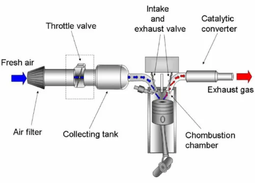
These systems improve the drivability and reduce the emissions. They introduced functionalities in automobiles that were not feasible with purely mechanical systems. All mechatronics management remains invisible for the customer and allows correction of systems in real time (engine management, stability control, braking control…). The modern Spark Ignition (SI) engines are equipped with mech-atronic components that control air-to-fuel ratio (George and Pecht 2014). The process of varying air intake into the engine cylinder is accomplished employing the Electronic Throttle Body (ETB). As shown in Figure 1-4, the throttle valve varies the quantity of air flow into the engine and thereby cylinder charge, which determines the engine torque (Rossi, Tilli et al. 2000). The ETB offers in acceleration maneuvers, a smoother vehicle behavior and ensures security by controlling the engine operation range (engine speed limitation, idle speed...) (Corno, Tanelli et al. 2011).

(31)

Figure 1-4. Electronic throttle body environment (Nentwig and Mercorelli 2008)

The ETB encompasses the aspects of a mechatronic system by containing mechanical parts, electric power, electronic sensor and a control system. Figure 1-5 details the composition of the ETB. A typical ETB includes a DC motor that actuates a gearbox and a valve. A potentiometer is generally used to measure the angle for control feedback. A failsafe system with two springs is used when the control system fails, it keeps the valve at the Limp Home position (between 10 deg and 14 deg) in order to provide the necessary flow to keep the engine running (Rossi, Tilli et al. 2000).

(32)

As reported by PSA and Valeo, the design of such system creates new challenges for the industrials because of its multi-physical aspect and the implication of different design teams (control, mechanic, electric, thermal, and fluid). Moreover, the nonlinearities of the system bring challenges in the design and the verification phases. A successful design requires a successful collaboration between multi-disciplinary teams. The ETB example will be used in this manuscript in the different chapters with different levels of maturity to concretize the design process of such components and validate our approach. The next section details the design process of mechatronic systems.

1.2 Design process for mechatronic systems

The ABET (Accreditation Board for Engineering and Technology, Inc.) definition of engineering design: “Engineering design is the process of devising a system, component, or process to meet de-sired needs. It is a decision-making process (often iterative), in which the basic sciences, mathematics, and engineering sciences are applied to convert resources optimally to meet these stated needs (Com-mission 1999)”. Like any design, the mechatronic design is an iterative procedure with defined steps. However, it is more complex than mono-disciplinary processes because it requires continuous inte-gration and collaboration. In this section, the main design cycles are analyzed.

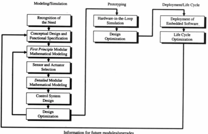
1.2.1 Sequential cycle

It is not uncommon to find companies that consider that mechatronics system design as a sequential cycle (Figure 1-6). This cycle consists of three consecutive phases: modeling and simulation, proto-typing and deployment. First, the requirements are analyzed and the conceptual design starts based on customer needs. The conceptual design aims to define the optimum configuration of the whole system without going into detail on its subsystems. The main functions are identified and an archi-tecture is created for the system. Then, a first modular mathematical model is created with the funda-mental behavior of the subsystems. After, a detailed model which is an extension of the first one provides more functions and accuracy for analysis. The control system is developed and the final step of this phase consists in the optimization of the system with its controller. If the requirements are designer can move the prototyping phase otherwise a new iteration is necessary to adjust the model.

(33)

Figure 1-6. Mechatronic sequential process (Shetty, Manzione et al. 2012)

The complexity of multidisciplinary design showed the limits of this approach. Downstream tasks are penalized because they are more and more constraints by the choices made during upstream tasks. In fact, the multidisciplinary optimum cannot be reached by successive monodisciplinary calculations. Moreover, the duration of the process is not optimal because the tasks are carried out one after an-other. Therefore, V-model which is more adapted for concurrent engineering was widely adopted by industrials (Shetty and Kolk 2010). Then, it was standardized for mechatronics in VDI 2206 guideline that will be presented in the next paragraph.

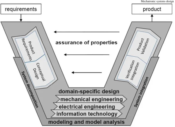
1.2.2 VDI 2206 cycle

The VDI 2206 guideline provides a design process which is more integrated than the sequential de-sign process. This cycle is divided into two phases: A top-down phase for system decomposition and a bottom-up for system integration (Figure 1-7). Even if the base of this process is sequential, the V-form highlights the continuous feedback connections between the two phases. The disciplines are

(34)

The customer requirements are identified in this step. A good understanding of customer requirements is the key to provide a suitable system (Wiesner, Freitag et al. 2015). Requirements should be clear and concise because this step is essential to have a first estimation of the resources and time allocation. Step2: Conceptual Design

Based on the requirements, system engineers identify the different functions of the system. This pro-vides a greater understanding of the system complexity. For each function, a functional subsystem is defined (Peluso 2015). Therefore, we can obtain different architectures depending on the chosen func-tional subsystems. Funcfunc-tional and architectural design can be combined into conceptual design (Kellner, Hehenberger et al. 2015). This step is important because it has a direct impact on the main parameters, properties, and cost.

Step3: Domain-specific Design

The detailed design step is between the two phases. The previously defined architecture is trans-formed into technical solutions with associating physical components to the functional subsystems. The architecture needs then to be modelled using embodiment tools. In this step, the system begins to take shape and first analyses are made to model the system (Törngren, Qamar et al. 2014).

Step4: Verification & Integration

Several analyses and simulations are made in this step to test the system against physical laws. The goal is to recompose the system and evaluate the integration of the different components (Petty 2009). The properties depending on the nature of the components (thermodynamic, vibration, dimensions...) and the requirements are verified and analyzed.

Step5: Product Validation

In this final step, the requirements related to the global system are validated. This validation can be experimental or virtual using analysis tools and multidisciplinary design optimization (Hammadi, Choley et al. 2012).

(35)

Figure 1-7. Design cycle of mechatronic systems (adapted from VDI Guideline)

1.2.3 Mechatronic design cycle in the industry

The VDI 2206 is, in practice, a spiraling process between decomposition phase and integration phase. We have initially incomplete requirements which gain completion during the decomposition phase. Also, conflicts in the integration phase lead to changes in the architecture defined by system engi-neers. The principle is to carry out in parallel different activities related to the product design. To study the mechatronic design cycle from an industrial perspective we decompose into SE, DE, and MDO (Figure 1-8). The predominant field in the first phase is SE which manages the decomposition activities (Requirements management, Functional modelling…). For the second phase, the field of DE is predominant. By DE we mean all the formal analyses and calculations made on CAD tools in the different disciplines involved in the mechatronic design (Embodiment, simulation…). Finally,

(36)

Figure 1-8. SE, DE, and MDO activities in mechatronic design

1.3 Systems Engineering (SE)

International Council on Systems Engineering (INCOSE) defines SE as “An interdisciplinary ap-proach and means to enable the realization of successful systems. It focuses on defining customer needs and required functionality early in the development cycle, documenting requirements, then proceeding with design synthesis and system validation while considering the complete problem. It integrates all the disciplines and specialty groups into a team effort forming a structured development process that proceeds from concept over production to operation. SE considers both the business and the technical needs of all customers with the goal of providing a quality product that meets the user needs” (Friedenthal, Griego et al. 2007). In this section, we will explore this field and its implication in the definition and decomposition phase.

1.3.1 Definition and decomposition phase

SE was developed to address the challenges of coordinating and managing the design cycle. It is typically viewed as a separate branch of engineering addressing both technical and management ac-tivities with the goal of balancing all project objectives. The system engineer intervenes concretely in the first part of the design cycle to define the system based on the requirements (Lightsey 2001). Therefore tools belonging to SE are tools for creating a common system model that integrates all partial models and their relationships (Biahmou 2015). SE focuses more on the process of designing a system rather than on the solutions to the design problem itself. It focuses on the system-level to

(37)

evaluate the properties of the system under consideration in order to ensure that the final system meets the design requirements.

There are various languages for SE (SysML, eFFBD, ISM…). Only the SysML language will be considered in this chapter because it is one of the most commonly used in industry.

1.3.2 SysML Language

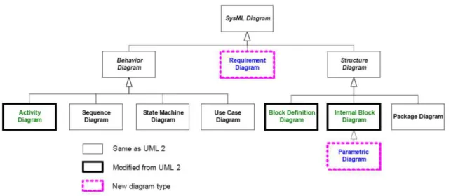
The System Modelling Language (SysML), comes from an effort from the International Council on Systems Engineering (InCoSE) and the Object Management Group (OMG) to integrate languages of different disciplines into one interdisciplinary language. SysML is the most widespread system mod-eling language in the industry and it derived from UML2.0 (Friedenthal, Moore et al. 2014). This language offers nine different diagram types representing various aspects of the system.

- Requirement diagrams are used to model the requirements, their organization and their re-lationships with the elements of the system.

- Activity diagrams allow modelling the chronological order of activities and decisions to model a process for example.

- Sequence diagrams are used to model the flow of control between actors and systems (blocks) or between parts of a system.

- State machine diagrams describe the states of a system and their changes in response to events.

- Use case diagrams describe the usage of a system by its actors (environment) and high-level services or features that the system has to offer.

- Block definition diagrams represent the structure of the system and provide an option for modelling the system hierarchy. The system consists of various blocks (modular units of the system), which are interconnected by connectors, which specify relationships between model elements, both within and across the boundary of the system.

- Internal block diagrams Represent the internal organization of a block and of its sub-blocks, and in particular the interconnections between the ports.

(38)

Figure 1-9. Diagrams of SysML language (Friedenthal, Moore et al. 2014)

The modelling of a system does not require the use of all the SysML diagrams, it depends on the type of study. To use this language efficiently in mechatronic design, we need methods to use the right diagram at the right moment.

1.3.3 Methods for SE in mechatronic design

As explained before, SysML language contains several diagrams that are linked to each other. A methodology is then needed to use them efficiently during the design cycle of mechatronic systems. “Black box” and “White box” approach was proposed for this purpose (Mhenni, Choley et al. 2014). In the first phase (Black box), the system is specified but not described by keeping an external point of view. The second phase (White box), the system is described in detail which corresponds to the conceptual phase. This methodology improves the traceability in the decomposition phase and pro-motes the diagrams reuse.

Figure 1-10. Black box-white box approach (Mhenni, Choley et al. 2014)

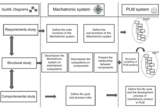
An integration modelling approach was also proposed in three steps (Abid, Pernelle et al. 2015). The first step is to define the system requirements with the external environment, main functions and link it to the PLM system. The second step is to study in detail the structure of the system with its subsys-tems and components. Finally, the behavioral study of the system allows defining the development process of the mechatronic system and its life cycle from PLM data (Figure 1-11)

(39)

Figure 1-11. Integration modeling approach (Abid, Pernelle et al. 2015)

1.3.4 ETB definition example

To illustrate the SE approach. Two diagrams of the ETB system will be presented here. The functional diagram as explained before shows the different functions of the system and the links between them (Figure 1-12). This diagram shows also the input and output of the system and its environment.

(40)

Figure 1-13. Two architectures of the ETB

In this manuscript, we will work with the standard architecture using a DC motor and a gearbox as shown in the BDD (Figure 1-14).

Figure 1-14. BDD of the standard ETB architecture

The decomposition of the system exposed in this paragraph is one of the main goals of the SE meth-odology. It gives a system level view of the product and organizes it in clear diagrams so that the disciplinary designers can refer to them. The next paragraph explains the current challenges of SE in industry.

1.3.5 SE challenges

These diagrams are only used to communicate between stakeholders and do not allow to make calcu-lations or to be simulated. The integration of simulation and analysis capabilities within SE is one of the most challenging and promising research activities. Such interest is also highlighted by the recent creation of “Systems Modeling & Simulation Working Group” (SMSWG) between the “International

(41)

Council on Systems Engineering” (INCOSE) and the “International Association of the Engineering Modelling, Analysis and Simulation Community” (NAFEMS). This recent cooperation highlights the fact that the integration between system level and multidisciplinary level environments is currently one of the most investigated areas of research (Cencetti 2016). The current lack of integration between them generates several problems during concurrent engineering. Iterations between system level and detailed level are difficult and design changes (which are more and more present) cannot be solved easily by disciplinary designers. The next section explains more this issue from the DE point of view.

1.4 Disciplinary Engineering (DE)

1.4.1 Integration and verification phase

DE is a technical and detailed work to create models and simulate the mechatronic system using mathematical and physical laws. This rigorous approach aims to optimize the system in its entirety and to generate all the necessary data to produce the mechatronic system. Design teams are brought to work together and to develop new ways of working to deal with conflicts that emerge during the integration. In each discipline, designers are working with specific tools and methods but they have to merge their work to verify the global system functionalities. Therefore, the main disciplines (me-chanic, electronic and control) are integrated depending on design maturity. This integration can be virtual by combining disciplinary tools or real by testing the control system with its structure (Figure 1-15). The main integration approaches in industry are:

- Model in the Loop (MiL): the plant model is connected to the controller model

- Software in the Loop (SiL): the plant model is connected to the controller translated C-code - Hardware in the Loop (HiL): the plant model interacts with the controller hardware

- Rapid Control Prototype (RCP): where the real plant is operated together with the simulated controller

(42)

Figure 1-15. Combining real and simulated parts in the mechatronic design (Isermann and Müller 2003)

The system integration comprises the spatial integration of the hardware components (actuator, trans-mission, cables, ECU…) and functional integration of software algorithms (control system, fault di-agnostic, HMI...). To sum up, integration in mechatronics means integration across traditional bound-aries. In the following, we detail the tools used in this phase.

1.4.2 DE tools

The tool landscape for developing mechatronic systems is large and diverse, consisting of a number of multi-domain tools and mono-domain tools. In one hand, multidomain tools take into account the functional and physical coupling between components. This level of modelling is usually done using 0D/1D models, represented by algebraic equations, ordinary differential equations (ODE) or differ-ential algebraic equations (DAE). These are some examples: Dymola, Open-modelica, Mobile VHDL-AMS, AMESIM, 20 SIM. On the other hand, Monodisciplinary tools are based on a 3D geo-metric representation. The monodomain phenomena are generally represented through partial differ-ential equations (PDE) and by using numerical approximations such as finite element methods (FEM). Here are some Mono-domain DE tools:

• In mechanical design, dimensions, shapes, and materials that correspond to the physical objects are the main interest. These are some examples: Solid Edge, SolidWorks, Catia.ProE

(43)

• Electronics deals with the physical implementation of the controller. The software packages for electronic design support predictions of behavior and execution time through logical and physical simulations.

• Electrical engineering commonly designs components to link electronic and mechanical domains like Synopsys, OrCad

• For specific physical phenomena, like thermal, fluid and magnetic effects, FEM tools based on mesh calculations are used. We can cite: Ansys, Abaqus, SiemensNX

• Test benches: Because no single model can ever flawlessly reproduce reality, there will always be an error between the behavior of a product model and the actual products. A test bench offers a real environment to verify the product in various conditions.

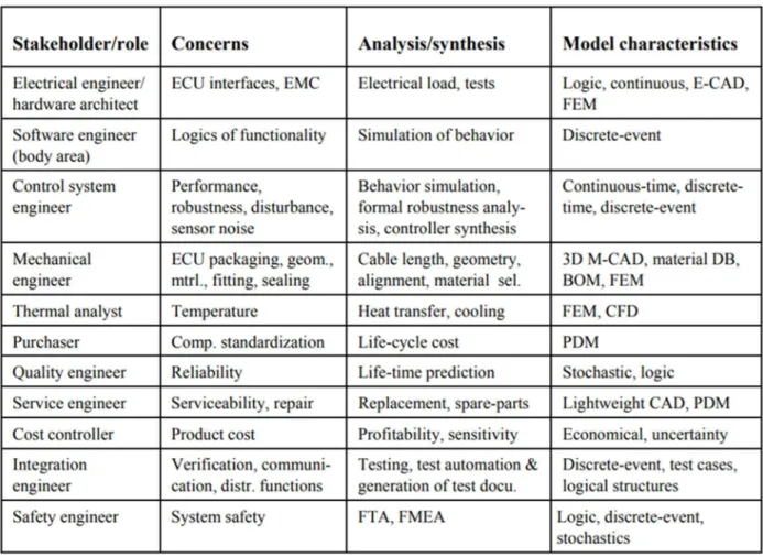
In this context, Table 1-1 summarizes the DE tools used in an automotive project.

(44)

Mono-domain tools perform well within their domains but cannot consider all the aspects of the mechatronic system. Multi-domain tools can cover different aspects of the mechatronic system but they are not accurate enough to perform the various steps of the design cycle and need enrichment from more accurate tools. Therefore, interoperability is necessary between these tools to realize the integration and the validation of the mechatronic system.

1.4.3 DE and interoperability

A multidisciplinary system is a source of complexity because designers from different teams struggle to communicate and find agreement on design decisions, each with their business constraints and conflicting objectives. Moreover, if a significant number of tools is proposed for multi-domain design mechatronic systems, these do not integrate all the stages of the design cycle (Cabrera, Foeken et al. 2010).

One possible solution to support communication is through data exchange standards. For instance, within the CAD community, a number of international standards have been developed to make prod-uct data exchange possible. Among these standards, the STEP standard (Pratt 2001) is the most re-nowned. Some key issues, such as errors in exchanged data and loss of data when using a standardized neutral model, are still not resolved (Gielingh 2008). As a result, organizations tend to rely on tools from a single vendor (which can be costly), or stick to documents and meetings for data exchange (which can be time-consuming).

Another solution is the Functional Mock-up Interface (FMI) which is an open standardized interface for co-simulation and model exchange between simulation tools (Nouidui, Wetter et al. 2014). The purpose of the standard is to allow models to be interchanged between different vendors, departments or modelling disciplines. Each sub-part can then be modelled in the most appropriate tool.

Finally, XML is a well-known exchange standard. The goal of XML is to enable the automated ex-change of content between heterogeneous information systems and thus to answer an interoperability problem. An XML document is a self-describing text file with tree-structured data. It is usable by any application but cannot support dynamic collaboration.

1.4.4 ETB open loop example

A simple example is presented in this paragraph to show some tools used in mechatronic multidisci-plinary design. The task is to improve an existing ETB (Bosch). The first model is an embodiment model in Catia (Figure 1-16).

(45)

Figure 1-16. 3D model of the ETB

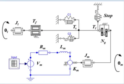
The architecture of the ETB and the involved parameters are detailed in Figure 1-17. The inertia of the valve, the gearbox as well as the gearbox ratio are calculated with the embodiment model to be used in the 0D model. The 0D model of the ETB is created using components from Modelica library (Figure 1-18). Initial values are given for the unknown parameters like the stiffness of the springs or the motor parameters. The list of the initial values is given in Table 1-1.Our goal is to understand the behavior of the system in open loop.

(46)

Figure 1-18. Modelica model of ETB in open loop Table 1-2. ETB initial parameters

Parameter Unit Description Initial value Motor

Km N.m/A Motor constant 0.02

Ke N.m.s/rad Back emf 0.02

Rm Ohm Resistance 1.5

Lm H Inductance 0.0015

Jm Kg.m² Inertia 4.8e-6

im A Current variable

Vm V Voltage variable

θ_m deg Motor angle variable

Gear

Ng - Ratio 20

Stop deg Angle interval [0,90] Load

(47)

Ts N.m Springs torque variable

Tf N.m Friction torque variable

Tl N.m Torque after reduction variable

C1 N.m/rad Main spring stiffness 0.3

C2 N.m/rad Limp home spring stiffness 0.6

θ_l deg Throttle angle variable

A simulation is made to understand the failsafe functionality. The failsafe system works when the control system of the ETB fails. It brings the valve to a pre-defined angle (limp home position), in order to provide the necessary air flow to keep the engine running. This position is between 10 deg and 15 deg depending on models. The limp home spring is connected to the lever and the sector gear, it works only when the lever is in contact with the stop limit. The main spring is connected to the sector gear and the mass. The role of the main spring (stiffness C1) is to bring the valve from open positon to limp home position. And the role of the second spring (stiffness C2) is to bring the valve from the closed position to the limp home position. In the two cases the equilibrium position is reached at the limp home position. The Figure 1-19 shows an example done with a throttle initially positioned at 90° with 0V supply voltage. The two springs reach the equilibrium position at 10deg.

(48)

This model gives us a first idea about the behavior of our system. We can understand how friction and springs work. However, this model needs optimization because the return time is too long. Opti-mizing such a model is difficult because we have conflicting parameters, if we reduce the main spring stiffness, the rising time will be shorter but the return time will be longer. Therefore, we need to use specific optimization methods. This challenge and others will be explained in the next paragraph. 1.4.5 DE challenges

Given the multidisciplinary nature of mechatronic design, engineers need diverse and heterogeneous DE tools. To integrate their work, engineers need communication means between these tools:

- The current interoperability solutions partially solve this need. They do not support the dy-namic exchange in concurrent engineering (Van 2006).

- The network-based Workflow Management (WfM) have until now been more used for man-aging business processes, documents flow, and much less engineering process (van der Aalst 2012).

- The Computer Supported Collaborative Work (CSCW) tools focus on communication fea-tures (messaging) and co-ordination (approval forms, workflow tools, videoconference tools) but few of them are interested in collaboration among actors (Pawlak 2010).

Besides, current engineering problems are increasingly characterized by a wide set of conflicting objectives that must be properly approached. The MDO was proposed for this purpose.

1.5 Multidisciplinary Design Optimization (MDO)

Multidisciplinary Design Optimization is “a methodology for a design of complex engineering sys-tems that are governed by mutually interacting physical phenomena and made up of distinct interact-ing subsystems (suitable for systems for which) in their design, everythinteract-ing influences everythinteract-ing else” (Sobieszczanski-Sobieski 1995). This methodology and its impact on mechatronic design are ex-plained in this section.

1.5.1 Problem formulation

In mechatronic design, problems are non-linear, have many constraints and require minimization of one or more criteria. Optimization algorithms have been developed to help the design team in this quest. The optimization is an important tool in decision science and in the analysis of physical sys-tems. To use this methodology, we must first identify the objectives to optimize and the constraints to respect. They depend on specific parameters, called Design Variables (DV). The aim is to find the

(49)

values for the DV that maximizes and minimizes the objective function with respecting the con-straints.

In mechatronic design, multidisciplinary models are involved in the design cycle with a strong inter-action between them. Therefore, optimizing a model without taking into account the others will gen-erate integration problems. The optimal design may even tend to converge on an absurd solution for the system (Chapman and Pinfol 2001). Given this state, MDO has been recognized as a promising solution to optimize globally the mechatronic system (Alexandrov 2005).

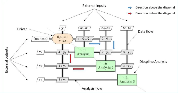
To express the MDO problem we use the All-At-Once formulation (AAO). This formulation contains all the coupling variables, their copies, state variables, consistency constraints and residual equations. The formulation of the other problems derive from this definition (Figure 1-20). For more details, readers can refer to (Cramer, Dennis et al. 1994).

(50)

presented in different manners. An interesting survey is provided in (Martins and Lambe 2013) where clear algorithms of these architectures are proposed to basically describe MDO architectures in uni-fied diagrams called XDSM (Figure 1-21). To read the diagram correctly, we have to follow the indicated numbers step by step. The directions of exchanging the parameters are illustrated in the Figure 1-21. The components consist of the discipline analyses represented by rectangles and a spe-cial component (driver) that controls the iteration which is represented by a rounded rectangle. The data flow is shown as thick gray lines. The components take data inputs from the vertical direction and output data in the horizontal direction. Thus, the connections above the diagonal flow from left to right and top to bottom, and the connections below the diagonal flow from right to left and bottom to top. The off-diagonal nodes in the shape of parallelograms are used to label the data. External inputs and outputs are placed on the outer edges of the diagram. The thin black lines show the driver process flow. Loops are represented by j → k with j < k. It means that if in the j step convergence condition is not reached we repeat again from the k step.

Figure 1-21. XDSM of a multidisciplinary analysis (MDA) process to solve a three-discipline coupled system

Two kinds of architecture can be found in the literature (Tedford and Martins 2010):

Monolevel approaches - The whole system is optimized using a single optimization process: • Multidisciplinary Design Analysis (MDA)

(51)

• Individual Discipline Feasible (IDF) • All-At-Once (AAO)

Multilevel approaches - Monodisciplinary optimizations are first conducted, before optimizing the whole system:

• Collaborative Optimization (CO)

• Concurrent SubSpace Optimization (CSSO) • Bi-Level Integrated Systems Synthesis (BLISS) • Analytical Target Cascading (ATC)

1.5.3 MDO tools

Unlike traditional optimization method, MDO is a multidisciplinary methodology (data analysis, vis-ualization, sensitivity analysis, optimization architecture…). MDO is accomplished by several types of software tools. Some CAD tools (Ansys, Matlab, Dymola..) can perform MDO. For instance, An-sys workbench proposes an MDO tool to optimize models in its environment. These MDO tools are limited because they cannot integrate external DE models and do not provide enough algorithms and features (meta-modelling, sensitivity, architectures…).

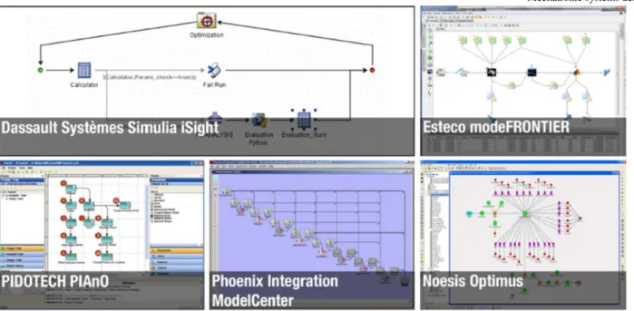
MDO can also be done by Process Integration and Design Optimization (PIDO) tools. They are spe-cialized in MDO and workflow management and offer various features to integrate DE tools in a common framework. Some examples are illustrated in Figure 1-22 (iSIGHT, modeFRONTIER, PAnO, ModelCenter, Optimus). They have relatively the same process: Optimization problem for-mulation, creating links between DE models involved in the loop and finally running the optimization algorithm and analyzing the results. Some associated techniques will be explained in the next para-graph.

(52)

Figure 1-22. Examples of PIDO frameworks

1.5.4 Associated techniques

When the MDO problem involves conflicting objectives, the algorithm identifies several solutions that are optimal considering the objective functions, they are called Pareto solutions. Figure 1-23 shows a Pareto front defining the solutions for two objectives (F1 and F2). The multi-objective opti-mization becomes more difficult with increasing number of objectives (Hammadi, Choley et al. 2012).

Figure 1-23. Pareto front in multi-objective optimization

Due to the presence of uncertainty, in real life optimization, it is often required to determine less sensitive solutions as robust designs (Figure 1-24). Robust solutions are areas in the search space

(53)

where significant changes in design variables produce only insignificant changes in the performance of the design. The challenge is to identify robust regions in the design space. Global and local opti-mums have to be taken into consideration in algorithm choice (gradient-based algorithms are sensitive to local optimums). The design space should be enlarged if the local optimum is not sufficient.

Figure 1-24. Robust vs local vs global optimum

In all the domains of engineering, designers use computationally expensive numerical models. The integration of such models in an optimization process can take a long time due to the significant number of iterations. Surrogate modeling is used in this case to make an approximation of the expen-sive model and then use it in the optimization process. In the field of surrogate modeling, three steps are required as we can see in Figure 1-25. An initial set of sample points is generated using a statistical method of Design of Experiment (DoE). These points are then used as inputs to run the simulation model and get function evaluations. Finally, a surrogate model type is selected to represent the re-sponse surface of the simulation model (Gaussian process (GP), polynomial regression, multi-variate adaptive regression splines (MARS)). If the precision of the model is not sufficient, new points are generated to adapt the model (Barton and Meckesheimer 2006).

(54)

Figure 1-25. The three steps of the surrogate modelling process

Another Surrogate modelling method appeared recently, called Space Mapping. The difference with the first approach is that we assume the existence of two models for the same system: a fine model (precise and expensive) and coarse model (cheaper and less accurate). The idea is to use the coarse model in the optimization process and to update it with the fine model to improve the accuracy (Figure 1-26). The algorithm establishes a mapping between the two models using Broyden updates (Bandler, Biernacki et al. 1994). The critical part of the process is the mapping function. Many techniques exist depending on the mapping function (Intput Space Mapping, Manifold Space Mapping, Agressive Space Mapping, Output Space Mapping).

Figure 1-26. Space mapping principle

1.5.5 ETB optimization example

The ETB model presented previously in paragraph 2.4.4 was not optimal. In this paragraph we try to optimize it following these specifications:

(55)

• The rising time (0° to 90°) should be lower than 150 ms (12V supply voltage)

• The return time with the failsafe system (90° to 10°) should be lower than 300ms (0V supply voltage and open circuit)

• The maximum torque of the throttle should be between 2N.m and 3.5N.m

The optimization problem presented contains two contradictory objectives because if we want to de-crease the return time we should use a spring with high stiffness and this will delay the rising time. Therefore, a multi-objective optimization is applied by combining Modelica with ModelCenter soft-ware. The optimization details are presented in Table 1-3.

Table 1-3. Optimization problem

Unit Lower bound Start value Upper bound Objectives to minimize Rize_time s - 0.24 0.15 Return_time s - 3.38 0.30 Problem Constraints Tl_max N.m 2 1.8 3.5 θ_max deg 89 90 91 Design Variables Km N.m/A 0.01 0.02 0.08 Rm Ohm 1 1.5 4 Ng - 15 20 30 C1 N.m/rad 0.1 0.3 1

(56)

Figure 1-27. Modelica model for optimization

To carry out the optimization, Modelica was combined with ModelCenter software (Figure 1-28). From the algorithms available in ModelCenter, we have chosen the NSGA II algorithm (Nondomi-nating Sorting Genetic Algorithm).

Figure 1-28. Optimization between modelica and ModelCenter software

Since the problem is multi-objective, the solution is not unique but we obtain a set of Pareto solutions. The Pareto Front is presented in the Figure 1-29. After 990 iterations, the solutions found present good performances and respect the torque constraint. The rising time can attend 118ms, the return time can attend 150ms and the designer should make the compromise between these two objectives. The torque value is in the range between 2N.m and 3.5N.m and this is sufficient to overcome the resistive torques (Mcharek, Hammadi et al. 2016).

(57)

Figure 1-29. Pareto Front solution

Four points are selected with the associated design variables in the Table 1-4.

Table 1-4. Four selected solutions

Unit 1 2 3 4 Objectives values Rizing_time ms 128 118 120 131 Return_time ms 206 302 190 250 Constraints values Tl_max N.m 2.0 2.8 2.1 2.3 θ_max deg 90 90 90 90 Design Variables

(58)

The solution 2 is then compared with the initial set for illustration as shown in Figure 1-30.

Figure 1-30. Comparison between the initial and the optimized set

1.5.6 MDO challenges

MDO is essential to the design and operation of a complex system. It has been successfully applied in the designs of many complex systems such as aircrafts, automobiles, shipbuilding, and civic infra-structures. However, industrial are still facing problems applying MDO due to:

- The difficulty of formalizing real problems into MDO problems. If the optimization problem is poorly defined, the goal will not be reached

- The difficulty to apply MDO on the integration phase due to the complexity of DE tools - The lack of human decision-making support and collaboration means in MDO as reported in

the NSF workshop

- The difficulty to integrate MDO to the design cycle

Regarding MDO challenges and those of SE and DE, we propose in the next section our research problematic.

(59)

1.6 Research problematic

1.6.1 Literature review

Design cycle is recognized as the primary contributor to the final product form, cost and reliability. The major opportunities for cost savings occur in this phase. There is a need to rapidly conduct design analyses involving multiple fields communicating together (Törngren, Qamar et al. 2014). Torry-Smith argues in his survey that the most reported challenges in mechatronic design are related to how information linked to the product concept can be shared across engineering disciplines (Torry-Smith, Qamar et al. 2013). We cannot share correctly the information across the design cycle or reuse effi-ciently previous works if SE, DE, and MDO are separated.

The fragmentation between SE and DE can be explained by:

- The nature of the results is different between the two fields (qualitative vs quantitative) (Simpson and Martins 2011).

- Different views and perspectives about the system (hierarchical decomposition vs disciplinary decomposition) (Zheng, Le Duigou et al. 2016).

- Incompatible tools used by system engineers (UML, SysML..) and disciplinary engineers (CAD, CAE, FEM..) (Borches and Bonnema 2010).

- Different capabilities between SE and DE (non-technical vs technical) (Price, Raghunathan et al. 2006).

The fragmentation between DE and MDO can be explained by:

- Different coupling methods between the analysis tools (semi-formal and manual vs formal and automatic) (Hiriyannaiah and Mocko 2008).

- Different strategies between DE and MDO (exploration vs optimization) (Simpson and Martins 2011).

- DE tools are tightly associated with a specific discipline but MDO are more generic and cut across disciplines (specific vs generic) (Simpson, Toropov et al. 2008).

(60)

and academic experts. It enables the industrial problems and requirements to be identified and dis-cussed. My research activities have always been linked to the meetings of MIMe projects and the feedbacks of the involved industrials. Here is a summary of the reflections constructed with the dif-ferent work packages:

WP1 – IT expertise

- Issues related to the database should be considered early in the conceptual phase of a collab-orative framework.

- The traceability of the exchanges during the collaboration is important for reuse. WP2 – KM expertise

- Traditional means of collaboration (emails, phone, visio…) are inadequate for concurrent en-gineering and reuse

- The semantic mismatch between stakeholders generates problems during collaboration phase. WP3 – SE expertise

- Communication between SE and DE is crucial for trade-offs and cannot be performed with the current tools.

- The need for dynamic verification of requirements during concurrent engineering. WP5 – Design process expertise

- When synchronizing MDO with the design cycle activities, how can we obtain the right results at the right moment?

- How can we ensure the collaboration between two companies having different PLM systems? - How can we reduce the design efforts in reuse phases?

All these points raise serious problems. The next paragraph presents our research problematic in this context.

1.6.3 Research problematic and objectives

The main goal of the design cycle is to realize in a short time a high-quality design solution that satisfies the customer requirements. Disciplinary engineers are at the center of this cycle, they use various heterogeneous tools. As we explained before, the collaboration between disciplinary engi-neers is not efficient and it is disconnected from SE and MDO (Figure 1-31). The problematic of this work can be summarized in two questions:

(61)

- Q1: How can we ensure a dynamic collaboration at the disciplinary level while remaining coherent with the system level?

- Q2: How can we formalize the knowledge generated during the collaborative design to facil-itate reuse and multidisciplinary design optimization?

(62)

(63)

Product Lifecycle Management

and Knowledge Management Solutions

The topic of knowledge management and the technologies associated are nowadays receiving ample attention, especially in mechatronic design. This chapter is devoted to the description of knowledge based solutions to support SE, DE, and MDO. This state of the art will be followed by a work positioning.