Constrained H̳₂ design via convex optimization with applications

Constrained 7t2 Design via Convex Optimization

with Applications

by

Beau V. Lintereur

B.S., Aeronautics and Astronautics Purdue University, 1996

SUBMITTED TO THE DEPARTMENT OF AERONAUTICS AND ASTRONAUTICS

IN PARTIAL FULFILLMENT OF THE REQUIREMENTS FOR THE DEGREE OF

Master of Science

at the

Massachusetts Institute of Technology

June, 1998

( 1998 Beau V. Lintereur. All rights reserved.

Signature of Author

Department of Aeronautics and Astronautics May 8, 1998

Approved by

Dr. Brent D. Appleby Charles Stark Draper Laboratory Thesis Supervisor

Certified by

Professor Eric Feron Assistant Professor of Aeronautics and Astronautics Thesis Advisor Accepted by MASSAC SETT an OFTECHNOL GY

JUL 8 1998

LIBRARIES

Professor Jaime Peraire Department Graduate Committee

nWaC#r

pea , ev 6s to reprodceaond to dbtftte pubcly pcper and

ekxfatrn coptes 1 thb Ws*

Constrained 7i

Design via Convex Optimization with

Applications

by

Beau V. Lintereur

Submitted to the Department of Aeronautics and Astronautics on May 8, 1998 in partial fulfillment of the

requirements for the degree of Master of Science

Abstract

A convex optimization controller design method is presented which minimizes the closed-loop 712 norm, subject to constraints on the magnitude of closed-loop transfer functions and transient responses due to specified inputs. This method uses direct parameter optimization of the closed-loop Youla or Q-parameter where the variables are the coefficients of a stable orthogonal basis. The basis is constructed using the recently rediscovered Generalized Orthonormal Basis Functions (GOBF) that have found application in system identification. It is proposed that many typical control specifications including robustness to modeling error and gain and phase margins can be posed with two simple constraints in the frequency and time domain. With some approximation, this formulation allows the controller design problem to be cast as a quadratic program.

Two example applications demonstrate the practical utility of this method for real systems. First this method is applied to the roll axis of the EOS-AM1 spacecraft attitude control system, with a set of performance and robustness specifications. The constrained 72 controller simultaneously meets the specifications where previous model-based control studies failed. Then a constrained 712 controller is designed for an active vibration isolation system for a spaceborne optical technology demonstration test stand. Mixed specifications are successfully incorporated into the design and the results are verified with experimental frequency data.

Thesis Supervisor: Dr. Brent D. Appleby Title: Senior Member of the Technical Staff

Thesis Advisor: Professor Eric Feron

Acknowledgments

Without a doubt, Lawrence McGovern deserves my greatest expression of gratitude and acknowledgment for the success of this work. From the earliest conceptual stages of this research to the final drafts of this thesis, Larry selflessly contributed his talents and time, and assumed a role equivalent to an academic advisor. Most remarkable is that Larry is a student himself with his own research interests and obligations. Although Larry is only a year my senior, he exhibits a combination of theoretical maturity and practical engineering know-how that is truly exceptional. His collabo-ration was paramount in developing and trouble-shooting the work presented in this thesis. As a bonus, Larry also turned me on to Jazz music which I will no doubt derive a lifetime of enjoyment.

I would like to thank Dr. Brent Appleby and Timothy Henderson at the Charles Stark Draper Laboratory. I always felt that Brent believed in this work and supported my interests. His ideas and contributions where timely and appropriate. It was Brent's idea to use the EOS-AM1 precision pointing attitude control problem as an design example. Tim Henderson encouraged the inclusion of the constrained 7i2

methodologies into the SCTB tools and provided the technical information required for the AVIS system identification and design example.

I thank Professor Feron at MIT for giving me the freedom to explore my research interests at Draper. His endless enthusiasm toward control and his research philoso-phies were always uplifting.

I want to thank the SCTB software development team which included Timo-thy Henderson, Michael Piedmont, Lawrence McGovern, and Jiann-Woei Jang for responding to my suggestions. Their work made my research more enjoyable and relevant.

I would like to thank my MIT/Draper friends Chris, Gordon, Rudy, Tony, George, Lisa, Larry and Steve (to name a few) for making every day in Cambridge seem like a Seinfeld episode.

Finally, I would like to thank my parents and my brothers Louis, Sam, Barry, Max, and Ross for their continued love, understanding and support. I owe a special thanks to my brother Louis who provided countless encouragement and advice through my engineering studies. His example has been inspirational.

This thesis was prepared at The Charles Stark Draper Laboratory, Inc., under Draper IR&D funding. Publication of this thesis does not constitute approval by Draper or the sponsoring agency of the findings or conclusions contained herein. It is published for the exchange and stimulation of ideas. Permission is hereby granted by the Author to the Massachusetts Institute of Technology to reproduce any or all of this thesis.

Contents

1 Introduction

1.1 Linear controller design overview . . . . 1.1.1 Classical methods ...

1.1.2 Traditional model-based methods 1.1.3 Parameter optimization methods 1.2 Scope and Contribution ...

1.3 Organization ...

2 Constrained "72 Design

2.1 Youla Parameterization ...

2.1.1 State-Space Model of the Youla Parameterization 2.1.2 Parameterization of Q(z) . . . . 2.2 7i2 Performance Objective ... 2.3 Closed-loop Specifications . . . . 2.3.1 Time-Domain Constraints . . . . 2.3.2 Frequency-Domain Constraints . . . . 2.4 Additional Topics ...

2.4.1 Constrained Augmentation Design . . . .

2.4.2 Quadratic Frequency Domain Constraints . . ..

2.4.3 Peak-to-Peak Constraints . . . . 2.4.4 A Phase Constraints ... 15 . . . . . 16 . . . . 16 . . . . . 17 . . . . . 18 . . . . 25 . . . . . . .. . . 26 29 . . . . . 31 . . . . . 32 . . . . . 34 . . . . . 35 . . . . . 36 . . . . . 36 . . . . . 37 . . . . . 39 . . . . . 39 . . . . . 41 . . . . . 43 . . . . . 44

3 Design Model and Linear Controller Design

3.1 The Design Model ...

3.2 Robustness to Modeling Uncertainty . . . .

3.3 Compensator Roll-off . ... 3.4 Loop Gain Roll-off ...

3.5 Gain and Phase Margin Constraints ...

Specifications

4 Generalized Orthonormal Basis Functions

4.1 Transfer Function Construction . . . . 4.1.1 _{Example Impulse and Frequency Response . . . .} 4.2 State-Space Realization: Direct Approach . . . . 4.2.1 _{First Order Pole Representation . . . .} 4.2.2 _{Second Order Pole Representation . . . .} 4.2.3 Series Interconnection . . . .

4.2.4 _{Special Case I.: Real Pole State-Space Representation . . .} 4.2.5 _{Special Case II.: Complex Pole State-Space Representation} 4.3 _{State-Space Realization: Balanced Approach . . . .}

4.3.1 _{Laguerre Function Balanced Realization . . . .} 4.3.2 Kautz Function Balanced Realization . . . . 4.3.3 State-Space Construction . . . . 4.4 Pole Selection for Design ...

4.5 System Identification Examples . . . . 4.5.1 Model-Matching with the GOBF . . . . 4.5.2 _{Frequency-Domain System Identification . . . .}

5 Graphical User Interface Tool

5.1 M ain Panel ... .. ... ... .... .. .. 5.2 Constrained Optimization Controller Design GUI . . . .

5.2.1 Objective Function Specification Mode . . . . 5.2.2 _{Basis Function Specification Mode . . . .} 5.2.3 Frequency-Domain Constraint Specification Mode

47 .. 47 .. 50 .. 51 53 54 61 63 65 65 67 68 69 71 71 72 74 75 75 76 78 78 82 87 .... . 88 . . . . . 88 . . . . . 89 . . . . . 89 . . . . . 91

5.2.4 Time-Domain Constraint Specification Mode . . . .

6 EOS-AM1 Precision Pointing

6.1 Classical Design... 6.2 Design Objectives ... 6.3 Design Model ... 6.4 Constrained 72 Design ... 6.5 Basis Selection ...

6.6 Compensator and Results . 6.7 Conclusion ... Attitude .,o°,. Control Example ... ... ... ... ... ...

7 AVIS Disturbance Rejection Control Example 7.1 Design Objectives ...

7.2 Design Model ... 7.3 Constrained 712 Design ...

7.4 Basis Selection ...

7.5 Compensator and Results . . . . 7.6 Conclusion ... 8 Conclusions 8.1 Future W ork . .. . . . . .. . . . . Bibliography 95 97 98 99 99 101 105 108 110 113 . . . . . 113 . . . . . 115 . . . . . 118 . .. .. 121 . . . . . 123 . ... . 125 129 131 133

List of Figures

1.1 Typical classical control loop. . ... ... 17

1.2 Traditional model-based method closed loop ... 17

1.3 Convex set ... 19

1.4 Convex function f. ... 19

1.5 Nonconvex, disconnected constraint set in controller optimization. .. 21

1.6 Intersection of convex constraint set and set of achievable closed loops in closed-loop optimization. ... 22

1.7 Convex constraint set in Q-parameter optimization. . ... 24

1.8 Organization of thesis. ... 27

2.1 Youla Parameterization. ... 31

2.2 All stabilizing compensators. . ... ... .. 33

2.3 T and Q interconnection ... 34

2.4 Exact magnitude constraint on H(w). . ... 38

2.5 Approximate magnitude constraint on H(w) with 8 linear constraints. 38 2.6 Nominal closed-loop system. ... ... . 40

2.7 Peak to peak constraint. ... 44

2.8 Phase change in lightly damped mode compared to damped mode... 45

3.1 Design m odel ... ... ... .... .. .. . . .. ... . . ... 48

3.2 Lower linear fractional transformation. . ... . 48

3.3 Disturbance rejection block diagram. . ... 49

3.4 Equivalent disturbance rejection block diagram. . ... 49

3.6 3.7 3.8 3.9 3.10 3.11 3.12 3.13 3.14 4.1 4.2 4.3 4.4 4.5 4.6 4.7 4.8 4.9 4.10 4.11 M ain panel. .. . .. . . . .. . . . ... Objective function control panel - 72 minimization.. . . . . . Basis function control panel ...

Frequency-domain constraint transfer function selection panel. Frequency-domain constraint tool . . . . .

Automatic constraint generator . . . . .

Roll-off constraint tool ...

Gain and phase margin constraint tool . . . . .

Multiplicative uncertainty (at plant output) . . . . .

Divisive uncertainty (at plant output) . . . . ...

Mixed uncertainty (at plant output) . . . . .

M ap of (1 + A)/(1 - A) ...

Guaranteed margins from constraints on mixed uncertainty . . . . .

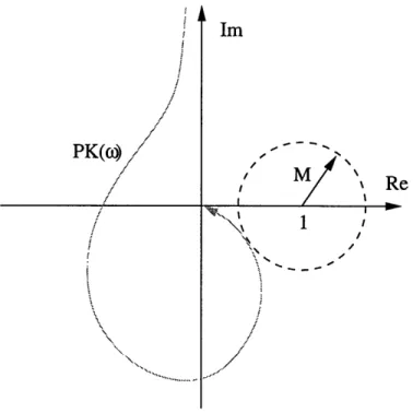
Guaranteed margins from constraints on multiplicative uncertainty. Guaranteed margins from constraints on divisive uncertainty . . . . . M-circle on Nyquist plot assuming positive feedback . . . . .

Example constraint on (1 + PK)/(1 - PK) at crossover frequencies. .

Example impulse response of the GOBF . . . . .

Example frequency response of the GOBF . . . . .

Series connection structure . ... First order pole block diagram ...

Second order pole block diagram . . . . ...

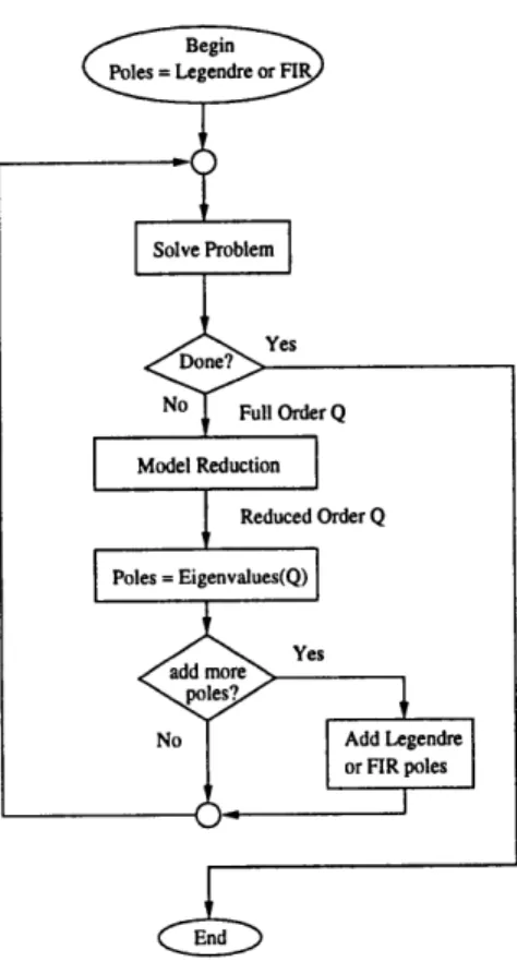
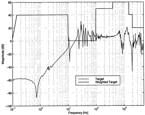
Recursive process for finding efficient GOBF for design . . . . Comparison of FIR, Laguerre, and GOBF approximations of H(z). Illustration of the 72 error vs. basis order with FIR, Laguerre, Random Real and Complex GOBF, and Recursive GOBF approximations of H(z). AVIS system identification example with GOBF.. . . . .. AVIS FRF magnitude and weighted magnitude . . . . .

AVIS system identification example with weighted GOBF ... .

5.1 5.2 5.3 5.4 5.5 5.6 5.7 5.8 ... . 89 . . . . 90 . . . . 91 . . . . 92 . . . . 93 . . . . 94 . .. . 94 . . . . 95

5.9 Time-domain constraint tool - Disturbance specification. ... 96

5.10 Time-domain constraint tool - Constraint specification. ... . 96

6.1 EOS-AM1 Spacecraft . ... .. .. 98

6.2 EOS-AM1 Design Model ... ... . 100

6.3 Orbital rate disturbance rejection constraint. . ... 102

6.4 Closed-loop transient response constraints. . ... . 102

6.5 Guaranteed gain and phase margins for bound on I(1+PK)/(1-PK)(w).103 6.6 Gain and phase margin constraints. ... ... 104

6.7 Robust stability constraints. ... 105

6.8 Legendre pole locations. ... 106

6.9 FIR pole locations. ... . ... 107

6.10 GOBF pole locations. ... ... 107

6.11 EOS-AM1 full and reduced order Legendre compensators compared to the classical design ... .... 108

6.12 Nichols chart of reduced Legendre and classical controllers. ... 109

6.13 Gain and phase margins of reduced Legendre controller... 109

7.1 Structural Test Model. ... ... 114

7.2 Strut #1 FRF data and plant model. . ... 116

7.3 Strut #1 system identification error at expected crossover range . ... 116

7.4 AVIS design model ... ... 117

7.5 AVIS frequency weights ... 118

7.6 AVIS disturbance isolation constraints and closed-loop performance.. 119

7.7 AVIS gain and phase margin constraints. . ... 120

7.8 Gain and phase crossover frequencies with reduced constrained 7-2 design.120 7.9 AVIS 20 dB/decade compensator roll-off constraints. . ... 121

7.10 Pole locations for 22nd and 27th order GOBF. . ... . 122

7.11 High frequency spiking in K/(1 - PK) with 100 order FIR basis. . . 124

7.12 Comparison of full and reduced order constrained 712 controllers with classical . . . . 126

7.13 Disturbance isolation comparison of classical and reduced order con-strained 7W2 design. ... 126 7.14 Gain and phase margins corresponding to 5 dB and 200 constraints

with reduced constrained 1i2 design; actual FRF based margins are 3

Chapter 1

Introduction

The linear controller design problem can be stated as follows: given a linear time invariant (LTI) model of a plant, find a controller that simultaneously meets a set of design specifications (and perhaps optimize a design metric) or determine that one does not exist. Historically, classical control methods have played a dominant role in practical control applications while model-based methods have been the focus of vigorous theoretical research. However, as many engineers have discovered, achieving a particular set of performance and robustness specifications with these methods can often be indirect. In recent years, the advancement in computer technology and efficient convex optimization algorithms has led to the reformulation of many control problems into general convex optimization problems [3, 4, 5, 60]. Some of the earliest related work is observed in the sequence of publications starting in 1964 by Fegley et. al. [6, 18, 19, 20, 44] where some control problems are shown to have linear and quadratic programming formulations. The result is that the most typical controller design constraints and objective can be cast as a convex optimization problem (frequently as a simple quadratic program) which can be solved efficiently. This ideology provides a nice foundation for developing general purpose Computer-Aided Design (CAD) software. The aim of this thesis is to develop a new CAD tool that extends the work of Boyd et. al. [3, 4], and Polak [60] which demonstrates through example the practical benefits of designing linear controllers with convex

1.1

Linear controller design overview

A brief overview and historical account of some analytic and optimization based linear controller design approaches are now discussed to add perspective to the current research. This overview also incorporates preliminary background material regarding mathematical programs, convexity, and optimization.

1.1.1

Classical methods

Traditional classical methods of solving the linear control design problem adopt the strategy of designing the loop gain, the plant and compensator serial combination

PK, and inferring the closed-loop performance. Often times the compensator is

as-sumed to have some fixed structure, such as a Proportional Integral Derivative (PID) or lead-lag structure, with corresponding gains that can be tuned through estab-lished rules, engineering intuition, or previous experience. Root-locus techniques, Nyquist diagrams, Bode plots, and Nichols charts are used to design the loop gain, analyze stability margins, and infer the closed-loop performance. This framework is especially suited for single-input/single-output (SISO) systems. Application of the classical methods to multiple-input/multiple-output (MIMO) systems is limited by the interplay or cross-coupling between the input/output channels.

A typical simplified control loop diagram used for classical synthesis is shown in Figure 1.1 where r, d, n, y, u, and e are various inputs and outputs that could represent the reference, disturbance, noise, measurement, control, or error signals respectively. Although there are multiple input/output locations in the typical clas-sical closed-loop diagram, each SISO closed-loop, for example from d to e, is treated separately. The designer must simultaneously consider the effects on all of the closed-loop transfer functions of interest when adjusting the compensator gains. Meeting multiple design objectives often becomes indirect and difficult because of the global influence of each gain. Furthermore, formulating the gain selection into an optimiza-tion problem results in a non-convex search space, as discussed in Secoptimiza-tion 1.1.3 under controller optimization methods, and has inherent practical limitations.

H

'U P y

KI

---_{I K r} I

- - - - - - - - - -

-Figure 1.1: Typical classical control Figure 1.2: Traditional model-based

loop. method closed loop.

1.1.2

Traditional model-based methods

Traditional model-based approaches such as the Linear Quadratic Gaussian (LQG, or

72) or '7o focus on finding analytic solutions to certain classes of problems. These

methods generalize the notion of the plant and closed loop as shown in Figure 1.2 so that closed loop H is a linear fractional transformation (LFT) of the plant P with the compensator K. This leaves the map H between the signals w and z open for minimization in terms of some metric or norm. Usually frequency weights or shaping filters are appended to these signals, for example W, and Wz in Figure 1.2, as a means of penalizing particular frequency bands or shaping the closed-loop response.

The optimal weighted 72 controller is found by

K = arg min JWzHW.1_{K 2},

where 11 112 is the system 2-norm. Similarly, the optimal W7. weighted controller is

found by

K = arg min IWzHW,, ,,

K

where 11- , is the system oo-norm. These problems are easily solved through two closed-form Riccati equations or by iterating over modified single parameter Riccati equations. The design variables are now the frequency weights or shaping filters W, and W,., and must be adjusted until the desirable closed-loop performance is achieved. One important advantage of this design framework is that MIMO systems are easily handled. However picking the correct set of weights or filters to simultaneously achieve

1.1.3

_{Parameter optimization methods}

The difficulties and limitations of traditional model-based and classical methods and the development of cheap and fast computers have motivated research in direct pa-rameter optimization design methods. The idea is to cast the linear controller design problem as a mathematical program of the form

min 4((w)

subject to w E 2

where ( is the objective function, w is the decision variables and Q is the feasible set. One important preliminary notion when considering parameter optimization methods or mathematical programs, is the nature of the feasible set and objective function. Most important is the notion of convexity.

A set Q is said to be convex if

Ax+(1-A)y E , Vx,yE Q, and0< A< 1.

This definition says that if the two points x and y are in the convex set, then any point on a line segment connecting x and y is also in the set as illustrated in Figure 1.3. A function f : f -+ R is said to be convex on a convex set Q if

f(Ax + (1 - A)y) _ Af(x)+ (1- A)f(y), Vx, y E , and 0 < A < 1.

This definition says that a line connecting two points f(x) and f(y) on a convex function lies above the function between the two points x and y as illustrated in

Figure 1.4.

A mathematical program is called convex if 4) is a convex function and Q is a con-vex set. One nice property of a concon-vex program is that the local optimal solution is also the global optimal solution. Two important special cases of convex mathematical programs are the linear and convex quadratic programs. In these special cases, the constraints that define the feasible set, also referred to as the constraint set, are linear scalar inequalities of the decision variables, while the objective function is either a linear or quadratic (positive definite) function of the decision variables respectively.

Xf(x)+(1- X)f(y)

Figure 1.3: Convex set Q. Figure 1.4: Convex function f.

Celebrated optimization algorithms used to solve the linear program are the Simplex Method [27] and the more recently developed interior point methods (for a survey of interior point methods see [22]). Reliable optimization algorithms to solve the quadratic program are readily available and described in [24]. More recent develop-ments in convex mathematical problems write the constraint set in terms of Linear Matrix Inequalities (LMI) [5] in which interior-point optimization methods have been developed to solve [51].

Non-convex optimization problems describe a class of problems where the objec-tive function and feasible set can be non-convex and even disconnected. In this case the nature of the objective function, feasible set, and the existence of local minimum can make these optimization problems NP-hard (A problem is NP-hard if solving it in polynomial time would make it possible to solve all other problems in the class of nondeterministic polynomial time problems in polynomial time).

The purpose of this section is to examine some of the proposed parameter opti-mization methods, and analyze their objective function and feasible set in terms of convexity and numerical tractability. The parameter optimization methods are cat-egorized into three classes determined by the design variable that is parameterized. The three most common choices are the compensator K, the closed loop H, or the Youla-Parameter Q. Similar survey discussions can be found in the work of Boyd et. al. [3, 4] and Polak [59].

Controller optimization methods

Possibly the most direct parameter optimization approach is to parameterize the com-pensator itself. This gives the designer maximum control over the comcom-pensator order and structure. In the work of Polak and Stimler [62], Davison and Ferguson [12], Ly et. al. [42] and Jacques and Ridgely [36], optimization-based design methods are derived where the compensator is parameterized directly. For example, one possi-ble parameterization for a discrete compensator could represent a partial fraction expansion

N bok + blk Z-1

K(z) , 1 + az - 1 _{+ a2k} - 2'

where the decision variables would be the coefficients bol, b02, ... , a2N. Similarly, the

compensator state-space could be parameterized in minimum-realization modal form as suggested in [42].

Now consider constraining a particular closed-loop transfer functions assuming a plant of the form,

P

P

P21 P22

with inputs w and u and outputs z and y as shown in Figure 1.2. The compensator appears in the closed loop in a linear fractional way

H = P11 + P12K(I - P22K)-'P21,

or in shorthand H = 7j(P, K). Hence a mathematical program constraining the set

closed-loops would be,

(P1) min 4(K)

KEICK

K = {K I P1 1 + P12K(I - P22K)-1P2 1 E CH}

where H is the closed-loop constraint set, IK is set of compensators that produce

closed loops inside the constraint set, and K is the compensator, parameterized in a finite dimensional space. Because of the linear fractional dependence of the closed loop on the compensator, convex constraints on the closed loop in general do not result in convex constraints on the compensator [4]. Figure 1.5 gives a graphical

Constraint Set on K Constraint Set on H

KK KH

LFr-K-Space H-Space

Figure 1.5: Nonconvex, disconnected constraint set in controller optimization.

interpretation of a possible constraint set on the compensator resulting from convex constraints on the closed loop. It is not hard to imagine why constrained optimization problems of this form quickly become numerically intractable. Never the less, some

CAD software exists to solve the linear controller design problem with controller

optimization formulations (it may be more relevant to solve the control problem this way for some systems). One example is the SANDY code of Ly [42]. There are many examples where these methods have been applied to controller design problems and compared to other parameter optimization methods. See for example [2, 37, 41, 47,

67, 69, 70].

Closed-loop optimization methods

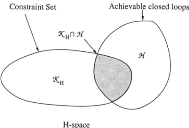
Another class of linear controller design problems treat the closed loop H as the design variable. Now a convex constraint set ICH of the closed loop avoids the complicated LFT map because the constraints and the design variable H are in the same space. Switching the design variable to the closed loop does not come free and requires ad-ditional interpolation conditions to ensure that closed loops in the constraint set are also achievable by some stabilizing compensator. The interpolation conditions ap-pear as additional linear scalar equality constraint in a mathematical problem [9]. In general, the interpolation conditions may result in an infinite number of equality con-straints. Figure 1.6 illustrates the convex intersection of the constraint set and set of

closed loops

H-space

Figure 1.6: Intersection of convex constraint set and set of achievable closed loops in closed-loop optimization.

achievable closed loops. The mathematical program associated with this formulation is

(P2) _{min 4(H),}

HEICHiti

where KfH _{is the closed-loop constraint set and 7- is the set of achievable closed loops.} ICH f w is an infinite dimensional space which is usually parameterized in a finite

number of dimensions.

Closed-loop optimization methods are proposed by Dahleh [9, 10] to solve the lI control problem, Elia to solve multi-objective control problems [16] and by McGov-ern [45] to solve the constrained 11 and -W2 _{problems. McGovern applied his method}

successfully to a real hardware system in [46]. The advantage of this method is that the constraints and the design variables are in the same space so the designer has max-imum insight into picking a good finite dimensional approximation for H. One disad-vantage of this method is that once a desirable closed loop is found, finding the com-pensator that achieves it relies on an inverse map through the Youla-Parameterization (described in the Q-parameter optimization methods section) , which could be nu-merically ill-conditioned. Furthermore, the addition of interpolation constraints adds complexity to the optimization problem, especially for multiblock problems [14].

Q-parameter optimization methods

The Q-parameter optimization method exploits the Youla or Q-parameterization of the close loop, eliminating the need for interpolation conditions. The Q-parameterization is an affine parameterization of the set of closed loops achievable with stabilizing com-pensators,

H = {T + T2QT3 I Q stable},

where T1, T2, and T3 are stable systems that are derived from the plant and Q is any stable realizable system. This parameterization was first recognized by Youla et. al. [71, 72] in 1976 and further developed in the 80's; see for example Desoer et. al. [13], Pernebo [57, 58], Nett et. al. [52], Doyle [15], Francis [21], and Vidyasagar [66]. With this formulation, a convex closed-loop constraint set is mapped to convex constraints on Q as illustrated in Figure 1.7. An important result of this parameterization is that every stabilizing compensator is related to Q through a bilinear map. Unfortunately general constraints on the compensator will result in non-convex constraints on Q. The mathematical program associated with this formulation is

(P3) min 4(Q)

QECQ

IQ, = {

QI

D(Q)

=

'(T + T2QT3),

where IC is the loop constraint set, KCQ is the set of Qs that produce closed-loops inside the constraint set, I) is the same objective function as in P2, and Q is the infinite dimensional design variable to be approximated with a finite dimensional parameterization.

Q-parameter optimization methods of design are proposed by Gustafson and Des-oer [25, 26], Hu and Loewen [30], Boyd et. al.[3, 4] and Polak and Salcudean [60]. In the work of Gustafson and Desoer and Hu and Loewen, convexity is sacrificed by assuming a general parameterization of Q where the design variables describe the loca-tion of the poles and zeros of Q. The CAD tool DELIGHT.MIMO [61] was developed

Constraint set on Q Constraint set on H

Affine map

Q-space H-space

Figure 1.7: Convex constraint set in Q-parameter optimization.

based on the non-convex formulation of Gustafson and Desoer while Hu and Loewen demonstrate their method using the MATLAB's Optimization Toolbox. By sac-rificing convexity, the designer has maximum control over the order and structure of Q and the resulting compensator. However in general, non-convex mathematical programs can quickly become intractable.

The approach proposed by Boyd et. al. and Polak uses a fixed denominator series expansion model to parameterize Q which preserves the convexity between the

Q-space and the parameter space defined by the decision variables. For example, assuming a SISO Q, a finite dimensional approximation of Q would have the form

N-1

Q(z) E F (z)0,,

n=O

where Fn(z) are some fixed denominator stable maps also known as basis functions,

N is the total number of basis functions and the Os are the decision variables. For

sufficiently large N this provides a good approximation for the space of Q but also results in high order compensators. Of course the choice of basis plays a significant role in approximating Q(z) with small N. Typically Q(z) is approximated with a Finite Impulse Response (FIR) basis. The CAD tool QDES [4] was developed based on this methodology and controllers designed with QDES have been demonstrated on a real hardware system [56]. Often times the resulting compensators are reduced using model reduction methods [48] before implementation.

1.2

Scope and Contribution

The goal of this thesis is to examine the impact of Q-parameterization optimization methods on practical control problems. The aim is to bridge the gap between theory and practice by developing a methodology that is accessible to the practicing design engineer. The method proposed in this work attempts to boost productivity by simplifying the problem formulation and user interface while employing proven and efficient optimization algorithms. Exploring more advanced formulations, for example using LMI's, which require more sophisticated optimization algorithms such as semi-definite programming is outside the scope of this work.

The main contribution of this thesis is a reduction in the control system design cycle time. The design cycle time is reduced by combining an easy to use problem specification interface with an efficient problem solution methodology. A more natural expression of many design specifications is proposed using two types of constraints in the frequency and time domain that are easily placed with the aid of a Graphical User Interface tool. The efficiency of the problem solution is increased by approximating the optimization problem with an easily solved quadratic program with a minimum number of basis functions (that are found through an ad hoc method developed in this work). A significant factor in realizing this contribution was incorporating the newly rediscovered Generalized Orthonormal Basis Functions (GOBF) into the Q approximation. The GOBF have mostly been studied for system identification appli-cations, however this work proposes that the GOBF are useful in the design problem as well. An ad hoc method for selecting the GOBF poles is proposed which is shown to produce lower order compensators while further improving the speed of finding an acceptable solution. This work demonstrates that Q-parameterization optimiza-tion methods are applicable to a variety of real controller design problems such as precision pointing attitude control of a flexible spacecraft or vibration isolation of a flexible space structure.

1.3

Organization

This thesis is organized into eight chapters as shown in Figure 1.8. The second through fourth chapters presents the developmental material for the constrained W-₂ design

methodology. In Chapter 2, the Youla parameterization of the closed loop is presented and the 72 _{objective function and closed-loop specifications in the frequency and time}

domains are formulated. Chapter 3 discusses how to build a good model for design and constrain it to achieve robustness to modeling uncertainty, compensator roll-off, loop gain roll-off, and gain and phase margins. Finally, Chapter 4 presents the Generalized Orthonormal Basis Functions (GOBF) that are used to approximate Q. Chapter 5 gives a brief overview of the Graphical User Interface (GUI) panels developed under subcontract for the Structural Control Toolbox (SCTB) [32] to illustrate how this methodology can be used in a general purpose linear controller design tool. Chapters 6 and 7 present real control applications where the constrained 712 method was used effectively. The GUI panels described in Chapter 5 were used to design the controllers in these chapters. Finally the conclusions and recommendations for future work are presented in Chapter 8.

Motivation, historical background, and preliminaries.

Design Model and Line; Design Specificat ~I ar Controller ions al _{- -} -Developmental material for contrained H 2 design.

Software description.

6 _{EOS-AM1 Precision Pointing} Attitude Control Example

---

-Design examples.

Conclusions and future work.

Figure 1.8: Organization of thesis.

2

3 4

Chapter 2

Constrained

'-12

Design

There are many variations to the constrained optimization problem that combine a particular objective function with a variety of meaningful constraint sets. In [4], the

W2, oo, and 11 objectives are considered with constraints such as asymptotic tracking,

decoupling, and regulation; overshoot, undershoot, and settling-time limits; bounds on closed-loop signal peaks; bounds on transfer function peak magnitudes; classical single-loop gain/phase margin (M-circle) constraints; and other miscellaneous bounds. Further variations on the constrained optimization design theme include methods that systematically incorporate a nominal controller into the formulation, which is necessary if the plant is unstable. The following discussion explores the marriage of the 7t2 (or LQG) design methodology and objective with two simple types of constraints in the frequency and time domain.

A constrained optimization method based on a nominal WH₂ design is appealing

for several reasons:

* The WU₂ objective function is easily constructed as a quadratic function of the

free parameters.

* A state space model for the Youla parameterization can be directly obtained from the controller and filter gains of a LQG design.

* An l12 design guarantees nominal stability of the plant given that the 72 design assumptions are met.

* Much research has been invested in designing 7-2 or LQG controllers.

The question often arises whether W'2 optimization is the best approach to use

if some nominally stabilizing controller already exists that exhibits marginal perfor-mance. The concern is that the constrained 7-2 formulation would start from scratch rather than exploit the good qualities of the nominal controller. The constrained augmentation method is developed in this chapter to deal with this issue.

To some extent, the objective function is less important than meeting a set of design constraints. A typical list of design specifications are usually constraints on the closed-loop and the compensator. Rarely are the specifications concerned with minimizing a closed-loop objective. Most design specifications are based on two simple types of constraints:

1. Time Domain. Constraints on the transient response z(t) to a specified com-mand or disturbance to remain within an envelope, i.e.,

Zmin(t) < z(t) Zmax (t) for a given w(t)

2. Frequency Domain. Constraints on the closed-loop gain at a particular fre-quency, i.e.,

IH(w)I < 7(w)

For example, frequency-domain constraints can be used directly or through small gains arguments for loop shaping, gain and phase margin constraints, and robustness to modeling uncertainty.

This chapter develops a powerful convex optimization controller design method to minimize the closed-loop 12 norm, subject to frequency and time domain constraints on the closed-loop system. Explicit equations are derived for the objective function and constraints. In addition, formulations for the controller augmentation design, quadratic frequency domain constraints, peak-to-peak constraints and A phase con-straints are included at the end of this chapter.

Figure 2.1: Youla Parameterization.

2.1

Youla Parameterization

The Youla parameterization of a closed-loop system is shown in Figure 2.1, where the closed-loop system H(z) = .7e(P, K) is a nz x n, system and K = Y(Ks, Q) is a nu x n, compensator. Furthermore, K, is a stabilizing controller with an observer-based state-space realization and Q is realizable and stable [43].

Typically, K, is derived from an observer based formulation where the output e is the measurement residual, and the input v is added to the actuator command signal. A well known result of observer theory is that the closed-loop transfer function from

v to e is zero. Because of this fact, an affine representation of all achievable H is:

H = {T + T2QT3 IQ stable}.

where T1, T2 and T3 are stable systems with sizes n, x nw, nz x nu, and ny x n, [72]. This powerful parameterization represents all stabilizing controllers as K = e(K,, Q) for some stable Q.

2.1.1

State-Space Model of the Youla Parameterization

State-space representations for K, and T are found in [3, 11, 43] and their derivations are reviewed here for completeness. Consider the plant:

P x[k] w[k] u[k] x[k + 1] A B1 B2 z[k] C, Dll D21

y [k] C2 D21 D22

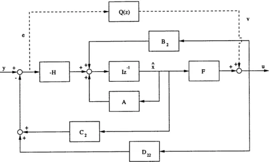
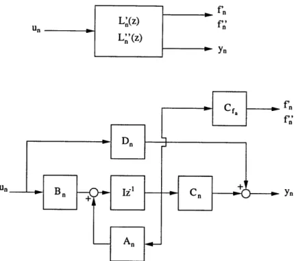
Figure 2.2 shows the structure of every linear, realizable, stabilizing compensator

K for plant P. The blocks connected by the solid line show the familiar

model-based controller structure of K, where F and H are the controller and filter gains respectively. When solving the discrete 7-2 control problem, these gains are computed

from the solutionI _{of two algebraic Riccati equations [73]. In Figure 2.2, the Youla}

parameter Q(z) is a proper and stable system with realization (Aq, Bq, C,, Dq). A derivation of K, is obtained directly from Figure 2.2 by adding the input v to the actuator command signal before the observer tap and tapping the output measurement residual to obtain e,

u[k] = Fi[k] + v[k],

e[k] = y[k] - C24 [k] - D22u[k].

In addition, a modification to the state estimate equation is needed to include the contribution of the signal v,

1[k + 1] = (A + B2F + HC2 + HD22F):[k] - Hy[k] + (B2 + HD22)v[k]. Combining these three equations, the state-space representation for K, immediately follows,

K, x[k] y[k) v[k]

x[k+l] A+B ₂F + HC₂+ HD₂₂F -H B₂+ _HD22

u[k] F 0 I

e[k] -(C2 + D22F) I -D22

1With the following assumptions: i) (A, B2, C2) must be stabilizable and detectable ii) Dll must

Q(z)

---I B 2

I I . +- : . A I +

Figure 2.2: All stabilizing compensators.

A realization for T is obtained by algebraically eliminating u and y in a lower linear

fractional transformation of P and K,,

T x[k] ,[k] w[k] v[k]

x[k +1] A + B2F -B 2F B1 B2 i[k + 1] 0 A+HC2 B1 + HD21 0

z[k] C1 + D12F -D 12F Dll D12

e[k] 0 C2 D21 0

where = x - &. Notice that the state estimate error , is uncontrollable from v while the state x is unobservable from the measurement residual e, hence the transfer function from v to e is zero. Figure 2.3 shows the interconnection between T and Q where the transfer function matrix T is a two by two matrix of the form,

T= .

ST

The closed loop from w to z is simply H(z) = .Fe(T, Q),

H(z) = T₁ + T2Q(I - T4Q 1T3.

Because the map from v to e (T4) is zero, H(z) is affine in

Q,

w z

Q(z)

Figure 2.3: T and Q interconnection.

with, ([A + B2F -B 2F B1 T = A+H 2

'

2.1.2

Parameterization of

Q(z)

An infinite-dimensional affine representation of Q(z) is given by:

nu ny oo

Q(z) = E

E

p=l q=1 n=O

where the Epq's are n, x ny matrices with the (p, q) entry 1 and all other entries zero,

{F,(z)} is a complete sequence of basis transfer functions, and the Opqn's are the free coefficients. A set of basis functions {Fn(z)} is complete if it spans the space of all stable realizable transfer functions, and is orthonormal if ECo fi[k]fj[k] = Jij, where

f,[k]

The above infinite-dimensional representation of Q(z) is approximated by the following finite-dimensional representation for optimization:

nu ny N-1

Q(z)

p=1 q=1 n=O

where N is the total number of basis functions. The basis functions have less impact on the approximation as n increases, hence good approximations can be achieved with sufficiently large N.

The FIR, Laguerre, and Kautz basis functions are examples of commonly used orthonormal basis functions, and have all been generalized by the following basis function model [54]:

(

z - G

k=0

-k

This construction allows for arbitrary placement of poles within the unit circle, rather than restricting pole placement to a single location as is the case with the FIR, Laguerre, and Kautz models. In [34], these functions are referred to as the Generalized Orthonormal Basis Functions (GOBF). The GOBF are discussed in Chapter 4 and explicit state-space realizations are provided.

2.2

7-2

Performance Objective

One of the most commonly used objective function in model-based control is the system 7t2 norm. The 7-2 norm of a MIMO system is defined as

I|H(z) 112 (Tr-

J

This system norm can be interpreted as the root mean squared value of the system output given a white Gaussian input. By Parseval's theorem, the 12 norm squared is approximately

nz nw L

i=1 j=1 k=O

where h[k] is the closed-loop impulse response and L is a finite but large number of time steps. The 7W2 norm of the closed loop is constructed from the Youla parame-terization in terms of the closed loop impulse response:

nu ny N-1

hij[k] = ti,ij [k]

+

=1 q=1 n=O

where f, is the basis function impulse response for Q, tl,ij, t2,ij, and t3,ij are the

number of basis functions. The 7W-2 suboptimal objective can now be written as a

quadratic function of qpq (a vectorization of ,pqn):

nu nly minimize

+

[

2.3

Closed-loop Specifications

2.3.1

Time-Domain Constraints

Specifications on the transient response of a system due to a specified input can be posed as a set of linear scalar constraints on Q. Consider a MIMO closed-loop transfer function H(z) in which a SISO transfer function Hij(z) is to be constrained. The output zij due to a specific disturbance wj is found by the convolution zij[k] =

(hij * wj)[k], where hij[k] is the impulse response of Hij(z). A constraint on the

transient response gl,ij[k] _ zij[k] _ gu,ij[k] can be written as

nu ny

E E(wj

p=l q=1

flu ny

Z

p=l q=1

where gl[k] and gu[k] are the lower and upper bounds of z[k]. This set of constraints is simply the linear inequality Atime 5 btime, where q is a vectorization of the Opq

2.3.2

Frequency-Domain Constraints

Consider the magnitude bound on the frequency response of a SISO transfer function in the MIMO system H(z):

with

n, ny N-1

H 3(z) = Tji + EEE T2,ipFqpqnT3,qj.

p=1 q=1 n=O

This constraint is equivalent to

R[Hij(w)]cosO + Q[Hij(w)] sinO < 'ij VO E [0,27r).

In [9], a magnitude constraint in this form is approximated by a finite number of linear constraints on the real and imaginary parts of Hij(w) by only considering a discrete number of angles 0_{n,N evenly spaced between 0 and 2r,}

7 2nr

R[Hij(w)]cos n,N+[Hij(w)] sin0 ,,N < Yij cos where On, = N ,n= 1, ... , N.

N N

The approximate constraint is easily visualized on a Nyquist plot of the constrained transfer function Hij(z). Figure 2.4 shows the exact constraint on the magnitude of

Hij(z). The approximation shown in Figure 2.5 corresponds to picking 8 discrete

lin-early spaced angles between 0 and 27r. Hence, in this example, 8 linear constraints are used to approximate a single frequency-domain constraint at a particular frequency.

This approximation has the property that the intersection of the linear constraints are contained within the exact constraint set. Define the compact set

S-_ {Hij(w) I Hij(w)j yjj(w)},

and the halfspace

2o,, - {Hij(w)

I

_![Hij(w)]

_<5

N

n

Re

Figure 2.4: Exact magnitude con-straint on H(w).

Figure 2.5: Approximate magnitude constraint on H(w) with 8 linear

con-straints.

as seen in Figure 2.5 for N = 8. It is easy to show that in the limit as N -+ oo

N

lim

n

The approximate magnitude constraint translates to a finite number of linear scalar constraints on q:

1 E(R[Sipqj(w)] cos On,N + .[Sipqj()] sin On,N)pq < Lij(w)

p=l q=1

where

Sipqj(w) = T2,ip(W)[ F0 (w) ... FN-1(W) _]T3,qj(W) and

Lij(w) = 7ij(w) cos - R[T,ij (w)] cos n,N - .,[Tij (w)] sin On,N.

This is simply the linear inequality Afreq¢ 5 bfreq, where q is a vectorization of the ,pq vectors.

2.4

Additional Topics

This section discusses alternate approaches to the constrained optimization problem. These topics represent ongoing ideas for further research, and will not be used in the examples.

2.4.1

Constrained Augmentation Design

In some cases an augmentation to an existing controller is preferred over a complete redesign. An example of this is a controller that operates in two modes where one is a low performance classical control mode and the other is a high performance aug-mented classical mode. For this case, the augmentation would simply provide the necessary correction to the nominal controller to meet the design specifications. A constrained augmentation approach is developed in this section so that augmenta-tions to existing nominally stabilizing compensators can be designed with the convex optimization framework.

The constrained augmentation design method is similar to the constrained 7-2

design method in that they both begin with a baseline stabilizing controller that is augmented with a stable Q parameter to satisfy some constraints set. The constrained augmentation approach departs from the traditional assumption that the baseline controller is observer based and exploits the Youla parameterization such that any stabilizing controller can be used. It is proposed that the objective function for the constrained augmentation method is constructed in a way that penalizes modifications to the baseline controller so that the desirable qualities of the baseline controller are preserved.

Modification to the Youla Parameterization

Frequently in control system development, a nominal controller has been designed which stabilizes the plant and achieves a modest level of performance or robustness. By exploiting the Youla parameterization, the nominal controller can be used as a starting point for an augmented control design. If the nominal controller is observer

Umodl U 1 I

I

I

L -I - n-o- - I

Figure 2.6: Nominal closed-loop system.

based (e.g., developed using LQG or Woo Riccati formulations), then the Youla pa-rameterization is simple as described in Section 2.1. On the other hand, if the nominal controller is not observer based, a Youla Parameterization can still be constructed as follows. Given the open loop plant:

z1

P11

P12

y P21 P22 U

add a modified control input to the actuator signal, and close the loop with the nominal controller, as shown in Figure 2.6. Then this "nominal" closed-loop can be

written as z T11 T12 yi T2 1 T2 2 Umod where T-1 = P1 1 + P12Knom(I- P22)-1P21 T12 = P 2 + P12Knom(I - P22Knom)- 1P22 T2 = (I - P22Knom)- 1 P21 T22 = (I - P22Knom) P22.

Because this new system is stable, an observer-based Youla parameterization can be constructed where the observer and state feedback gains are zero matrices (the feedback gains are no longer needed to stabilize the system). Defining this "sta-bilizing" controller with zero gain to be K,mod, the augmented controller is then

K = Knom + e(Ks,mod, Q). In this case, it can be shown that the Youla

Parameteri-zation reduces to:

H(z) = T11 + T12QT21

Q Minimization Performance Objective

It is not clear which objective function is best for constrained augmentation design. It is assumed that the designer has a good nominal controller and desires to modify it slightly while preserving its good qualities. In this case, it makes sense to penalize

modifications to the nominal controller. Minimizing the unweighted 72 norm of Q is one naive but simple way of implementing this strategy. That way, in the limit as IIQ(z)l1 goes to zero, the augmented controller converges to the original nominal controller. If the selected set of basis functions are orthonormal, the 712 norm of Q(z) is found by

n, ny N-1

IIQ(z)ll

Z Z

The 7-2 suboptimal Q objective can now be written:

minimize T

where q is a vectorization of Oi j

k-Design Specifications

The frequency and time-domain constraints are unchanged by the constrained aug-mentation design method.

2.4.2 Quadratic Frequency Domain Constraints

Some designers may prefer to write frequency-domain constraints exactly instead of using the approximation presented in Section 2.3.2. This section shows that a frequency-domain constraint can be written exactly as one quadratic constraint. The advantages of representation over the linear approximation are obvious: (1) it is

exact, (2) each frequency constraint can be represented by a single quadratic con-straint. However, it is unclear whether one quadratic constraint will perform better than N approximate linear constraints in the optimization algorithm. MINOS uses a projected augmented Lagrangian algorithm [24] to solve problems with nonlinear constraints. MINOS becomes more efficient solving nonlinear constrained problems if the gradient2 of the constraint equations are provided, otherwise they are computed numerically at additional computational cost. For this reason, both the quadratic constraints and the gradients are provided in this section.

The frequency-domain constraint, JHij(w)l 7ij(w) is most naturally written as

a single quadratic constraint. Define the scalar values a and /,

a Re[Hij(w)] P Im[Hij(w)].

Then the exact frequency-domain constraint shown in Figure 2.4 is,

a+2 + 2 < 2.

This constraint translates to a quadratic constraint on € by the following procedure.

nu ny N-1

a = Re [TI,ij(w)] + Re E T2,ip(w)Fn(w)T3,qj(w) Opqn

[p=1 q=1 n=O nl ny N-1

3

E E

where [1,1,0o 1,1,1 ... on,ny,N-1 _]T and

ba = Re [T,j (w)]

An - Re[(W T2,ip(wFn 3(wT,qj ) T

bo ' Im [T,ij(w)]

A Im

[

Now the quadratic constraint on 0 can be written,

T ( T + A3A T o +2T +2

(AA, + ApA ) + 2¢T(AabQ + Apb,) + be + bo < '2 and the gradient d( 0 + 2) is easily computed by,

(a2 2) _{= 2ATa + 2AP.}

Experience using quadratic constraints in the constrained 7i2 problem is limited. In the few examples that quadratic constraints were tried, MINOS was less robust in

terms of finding an initial feasible solution than when solving the problem with the linear approximation constraints.

2.4.3

Peak-to-Peak Constraints

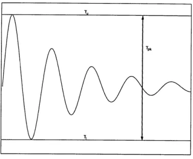
Peak-to-peak constraints on transient responses due to specified inputs are a compact way to write some time-domain specifications. A more attractive application of these constraints is the potential for optimizing the peak-to-peak value. For example, a specification that wishes to minimize the excursion of a state from the origin, as in a disturbance rejection or tracking error problem, would be easily posed as a peak-to-peak constraint, where the constraint value is actually included in the objective function for minimization.

A peak-to-peak constraint on the transient response to a fixed input as shown in Figure 2.7 is easily formulated with the addition of two variables 7, and 71. The response zij and the variables are constrained in the following way:

zij < Yu

zij > 'Yi

N- Y1 < 7pk,

where zij[k] = (hij * wj)[k] and Ypk is the peak-to-peak constraint value which can be fixed or a variable. To implement this in the optimization problem, the first two inequalities are treated like time-domain constraints with the exception that y, and

Figure 2.7: Peak to peak constraint.

-y are decision variables like 0 instead of constants but are not represented in the

objective function. The last inequality is in the correct form for the optimization problem. It is up to the designer to determine whether 7pk is best defined as a fixed value or a variable that is included in the objective function.

2.4.4

A Phase Constraints

A constraint on the phase change between two frequencies is one way to increase

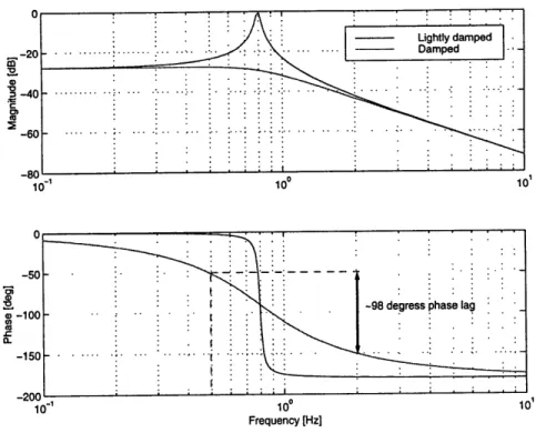
damping in a closed-loop mode. The phase change of a lightly damped mode is much more dramatic in the neighborhood of the resonance frequency than in a damped mode. This is illustrated in Figure 2.8 where two modes with a natural frequency of 0.796 Hz but with different damping ratios are plotted. The lightly damped mode has a damping ratio of 0.02 and experiences nearly 1800 of phase lag between 0.5 and 2 Hz, while the damped mode with damping ratio 0.6038 only experiences roughly 980 of phase lag. Hence, constraining the phase lag between two frequencies can be used as a mechanism for constraining the damping. These constraints were motivated as a method to eliminate the spiking effect described later in Section 7.4 and shown in Figure 7.11, where mismatched lightly damped poles and zeros cause large gain and phase changes in the closed-loop.

Lightly damped .... ... . . . .... Damped M -40 . -60--80 10-1 10o 10 50

-S1 -98 degress phase lag

( -100

150

--200

10-1 100 10

Frequency [Hz]

Figure 2.8: Phase change in lightly damped mode compared to damped mode.

The phase change between two frequency points can be written as a quadratic constraint by exploiting the fact that [8],

arg = argz - argz2,

where z E C and argz = tan-1(Im{z}/Re{z}). The change in phase of a closed-loop transfer function Hij(z) between two frequency points is equivalently written,

AO = 01 -2 = Hij(

Hij (W2)

where 0 = LHij(w), Hij(w) = a + iP, and a and 0 assume the same definitions as in Section 2.4.2. After some algebra an inequality constraint can be written,

AO = tan- 1 a,2,- a0f 1 <

1aa2 + /102

-where 7 is the constraint on the change of phase. Finally, the constraint is written,

(al02 - a₂ 1) - (ala2 + 012) tan y < 0,

where a and

/