Deformation-invariant sparse coding

(1)

Deformation-Invariant Sparse Coding

by

George H. Chen

B.S., Electrical Engineering and Computer Sciences, UC Berkeley, 2010 B.S., Engineering Mathematics and Statistics, UC Berkeley, 2010

Submitted to the Department of Electrical Engineering and Computer Science in partial fulfillment of the requirements for the degree of

Master of Science

in Electrical Engineering and Computer Science at the Massachusetts Institute of Technology

June 2012

@

JUL

0 1 2012

LIBRARIES

Signature of Author:

Department of Electrical Engineering and

Certified by:

Associate Professor of Electrical Engineering and

rs George H. Chen Computer Science May 23, 2012 Polina Golland Computer Science Thesis Supervisor Accepted by:

Professor of Electrical Engineering Chair, Committee

Leslie A. Kolodziejski and Computer Science for Graduate Students

I

(2)

(3)

-Deformation- Invariant Sparse Coding

by George H. Chen

Submitted to the Department of Electrical Engineering and Computer Science in partial fulfillment of the requirements for the degree of

Master of Science

Abstract

Sparse coding represents input signals each as a sparse linear combination of a set of basis or dictionary elements where sparsity encourages representing each input signal with a few of the most indicative dictionary elements. In this thesis, we extend sparse coding to allow dictionary elements to undergo deformations, resulting in a general probabilistic model and accompanying inference algorithm for estimating sparse linear combination weights, dictionary elements, and deformations.

We apply our proposed method on functional magnetic resonance imaging (fMRI) data, where the locations of functional regions in the brain evoked by a specific cognitive task may vary across individuals relative to anatomy. For a language fMRI study, our method identifies activation regions that agree with known literature on language processing. Furthermore, the deformations learned by our inference algorithm produce more robust group-level effects than anatomical alignment alone.

Thesis Supervisor: Polina Golland

Title: Associate Professor of Electrical Engineering and Computer Science

(4)

(5)

Acknowledgements

The past two years have been a tumultuous success, thanks to an incredible cast of people who've helped me along the way. At the forefront of this cast is Polina Golland, who has been a phenomenal advisor. Polina has provided me insight into a slew of problems, and I've lost count of how many times I've crashed into a road block, she'd suggest a way to visualize data for debugging, and-voilh-road block demolished! At the same time, Polina has been tremendously chill, letting me toil at my own pace while I sporadically derail myself with side interests divergent from the Golland group. Thanks Polina, and thanks for ensuring that I don't derail myself too much!

This thesis would not have seen the light of day without the assistance of my collab-orators Ev Fedorenko and Nancy Kanwisher. As I have no background in neuroscience, Ev and Nancy were instrumental in explaining some of the basics and offered invaluable comments, feedback, and data on the neuroscience application that drives this thesis. It really was the neuroscience application that led to the main model proposed in this thesis rather than the other way around.

Meanwhile, landing in Polina's group was a culture shock in itself as my background was not in medical imaging. Luckily, members of the group have been more than ac-commodating. Without the patience of former group members Danial Lashkari, Gabriel Tobon, and Michal Depa in answering my barrage of questions on functional magnetic resonance imaging and image registration during my first year, my transition into work-ing in medical imagwork-ing would have taken substantially longer with at least a tenfold increase in headaches, futility, and despair. I would also like to thank the rest of the group members for far too many delightful conversations and for putting up with my recurring bouts of frustration and fist shaking. Numerous thanks also go out to visiting group members Rene Donner, who hosted me in Austria, and Prof. Georg Langs, whose bicycle that I'm still borrowing has immensely improved my quality of life.

(6)

Many students outside of Polina's group have also had a remarkable impact on my education and crusade against grad-student-depressionitis. Eric Trieu has been a repository of great conversations, puns, and medical advice. James Saunderson has been my encyclopedia for math and optimization. As for machine learning, I have yet to meet any grad student who has amassed more machine learning knowledge and big-picture understanding than Roger Grosse, who persistently is rewarding to bounce ideas off of. I also want to thank the rest of the computer vision and Stochastic Systems Group students for all the productive discussions as well as new ways to procrastinate. To solidify my understanding of probabilistic graphical models, I had the fortune of being a teaching assistant for Devavrat Shah and Greg Wornell, who were an absolute riot to work with. Too often, their perspectives on problems led me to all sorts of new intuitions and epiphanies. Many thanks also go to my co-TA's Roger Grosse (again) and George Tucker, who contributed to my project of making Khan Academy style videos for the students. I still can't believe we threw together all those videos and churned out the first ever complete set of typeset lecture notes for 6.438!

Outside of academics, I've had the pleasure and extraordinary experience of being an officer in the Sidney Pacific Graduate Residence. I would like to thank all the other officers who helped me serve the full palate of artsy, marginally educational, and down-right outrageous competitive dorm events throughout the 2011-2012 academic year, and all the residents who participated, not realizing that they were actually helpless test subjects. My only hope is that I didn't accidentally deplete all the dorm funds. I would especially like to thank Brian Spatocco for being an exceptional mentor and collaborator, helping me become a far better event organizer than I imagined myself being at the start of grad school.

(7)

List of Figures

1.1 Toy example observed signals. . . . . 11

1.2 Toy example average signal. . . . . 12

1.3 Toy example observed signals that have undergone shifts. . . . . 12

1.4 Toy example average of the shifted signals. . . . . 13

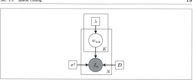
2.1 A probabilistic graphical model for sparse coding. . . . . 19

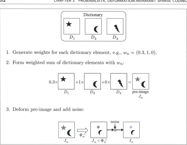
3.1 Illustration of how our generative model produces observed image I for a given dictionary of size K = 3. . . . . 32

3.2 A probabilistic graphical model for our generative process. . . . . 33

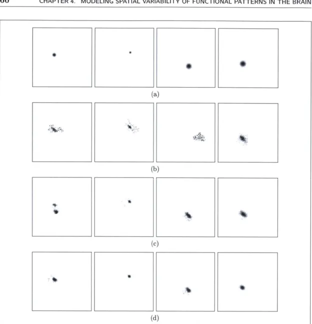
4.1 The synthetic data's (a) true dictionary, and estimated dictionaries us-ing (b) the watershed baseline, (c) the sparse codus-ing baseline, and (d) deformation-invariant sparse coding. . . . . 60

4.2 Synthetic data examples of pre-images and their corresponding observed images. All images are shown with the same intensity scale. . . . . 61

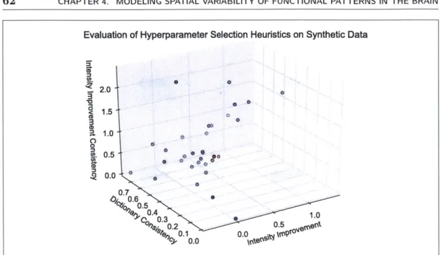
4.3 Synthetic data average of test images (a) without deformations, and (b) aligned with deformations estimated from training data using deformation-invariant sparse coding. Both images are shown with the same intensity scale and zoom ed in. . . . . 4.4 Scatter plot used to evaluate hyperparameter selection heuristics for syn-thetic data. Each hyperparameter setting (a,

#,

-y) is depicted as a single point, where a,

#,

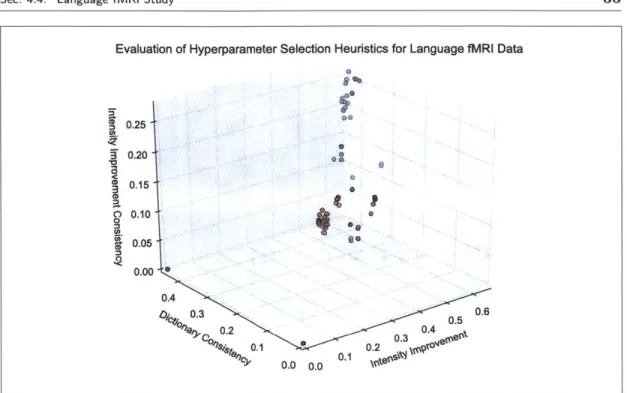
7y E {0, 102, 104, 106}. The top 5 hyperparameter set-tings (some overlap in the plot) according to our group average error on test data are shown in red; all other hyperparameter settings are shown in b lu e. . . . . 62

(10)

4.5 Scatter plot used to evaluate hyperparameter selection heuristics for lan-guage fMRI data. Each hyperparameter setting (a, ,y) is depicted as a single point, where a, 3, -y E {0, 102, 104, 106, 108. Hyperparam-eter settings in red and green have comparable dictionary consistency,

't intensity-improvement-difference < 0.1, and Wintensity-improvement > 0.4.

Hy-perparameter settings in green further achieve Nintensity-improvement > 0.6. 65 4.6 Estimated dictionary. (a) Four slices of a map showing the spatial

sup-port of the extracted dictionary elements. Different colors correspond to distinct dictionary elements where there is some overlap between dictio-nary elements. From left to right: left frontal lobe and temporal regions, medial prefrontal cortex and posterior cingulate/precuneus, right cere-bellum, and right temporal lobe. Dictionary element indices correspond to those in Fig. 4.7. (b) A single slice from three different estimated dictionary elements where relative intensity varies from high (red) to low (blue). From left to right: left posterior temporal lobe, left anterior temporal lobe, left inferior frontal gyrus. . . . . 66 4.7 Box plots of top 25% weighted random effects analysis significance

val-ues within dictionary element supports. For each dictionary element, "A" refers to anatomical alignment, and "F" refers to alignment via de-formations learned by our model. . . . . 66 4.8 Box plots of top 50% weighted random effects analysis significance

val-ues within dictionary element supports. For each dictionary element,

"A" refers to anatomical alignment, and "F" refers to alignment via de-formations learned by our model. . . . . 67 4.9 Box plots of top 1% weighted random effects analysis significance values

within dictionary element supports. For each dictionary element, "A"

refers to anatomical alignment, and "F" refers to alignment via

(11)

Chapter 1 Introduction

F

INDING _{glean high-level features in data. For example, an image may be represented as a}succinct representations for signals such as images and audio enable us to sum of a small number of edges or patches, and the presence of certain edges and patches may be used as features for object recognition. As another example, given a household's electricity usage over time, representing this signal as a sum of contributions from different electrical devices could allow us to pinpoint the culprits for a high electricity bill. These scenarios exemplify sparse coding, which refers to representing an input signal as a sparse linear combination of basis or dictionary elements, where sparsity selects the most indicative dictionary elements that explain our data. The focus of this thesis is on estimating these dictionary elements and, in particular, extending sparse coding to allow dictionary elements to undergo potentially nonlinear deformations.

To illustrate what we seek to achieve with our proposed model, we provide the following toy example. Suppose we observe the two signals shown below:

11

-10 -5 0 5 10 -10 -5 0 5 10

(a) Signal 1 (b) Signal 2

(12)

We imagine these were generated by including a box and a Gaussian bump except that they have different heights and the signal has been shifted left or right. If we don't actually know that the true shapes are a box and a Gaussian bump and we want to estimate these shapes, then a naive approach is to make an estimate based on the average of the observed signals:

1~

1.1

Figure 1.2: Toy example average signal.

For example, we could estimate the two underlying shapes to be the two-box mixture and the two-Gaussian-bump mixture shown above, which unfortunately don't resemble a single box and a single Gaussian bump. We could instead first align the observed signals to obtain the following shifted signals:

1.0 0.8 0.6 0.4 10 -10 -5 0 (b) Shifted Signal 2 5 10

Figure 1.3: Toy example observed signals that have undergone shifts.

0.8-0.6 -0.4 0.2 -10 -5 0 -10 -5 0 5

(a) Shifted Signal 1

(13)

13

Then the average of these shifted signals looks as follows:

1.0 0.8 0.6 0.4 0.2 -10 -5 0 5 10

Figure 1.4: Toy example average of the shifted signals.

From the average of the shifted signals, we can recover the box and the Gaussian bump! Moreover, the peak values in the box and the Gaussian bump are, respectively, higher than the peak values in the two-box mixture and the two-Gaussian-bump mixture in Fig. 1.2, which can be viewed as a result of destructive interference in the case where we don't align the signals before averaging. Generalizing from this toy example, this thesis looks at the problem of taking as input a set of images and producing as output a dictionary (e.g., a box and a Gaussian bump in the above example) and an ensemble of deformations (which could be much more complicated then shifts) to better align the images.

The key motivating application driving this thesis is the fundamental problem in neuroscience of understanding functional organization of the brain. Mapping out where different functions, such as language processing and face recognition, evoke activations in the brain provides insight into how we as a species perform day-to-day tasks and how abnormalities in these functional locations relate to neurological disorders. But arriving at any such population-level theory of functional organization of the brain demands that we find correspondences between activation patterns evoked by a specific function across different people's brains. We cast this problem of finding correspondences between functional activation regions across individuals as a sparse coding problem where we want dictionary elements to correspond to group-level functional units in the brain, which refer to brain regions consistently activated by a specific task across individuals. The problem with just applying sparse coding without incorporating deformations and hoping that the dictionary elements correspond to group-level functional units is twofold. First, people's brains vary anatomically, so images of different people's brains

(14)

don't line up perfectly. However, even if we account for this anatomical variability by first pre-aligning the brains to be in the same common anatomically-normalized space, when given the same stimulus such as a sentence to read, different people's brains will exhibit activations in different locations in the normalized space! This problem of spa-tial variability of functional activation patterns suggests that a possible solution is to model functional units as dictionary elements that deform into the space of each indi-vidual's brain. This leads us naturally to deformation-invariant sparse coding, where we estimate dictionary elements that may undergo deformations, so each dictionary ele-ment is unique up to a deformation. Of course, these deformations can't be too drastic, deforming, say, a disk into any arbitrary shape.

The main contributions of this thesis are as follows:

" We formulate a probabilistic model for deformation-invariant sparse coding and nrovide an accompanying inference algorithm that alternates between estimating

sparse linear combination weights, deformations, and dictionary elements. For estimating each deformation, the inference algorithm can use a broad class of existing image registration algorithms, i.e., algorithms for aligning two different images. We interpret our inference algorithm as a way to align a group of images while applying spatially-adaptive intensity equalization per image.

" We demonstrate deformation-invariant sparse coding on neuroimaging data from a language study. Our method identifies activation regions that agree with known literature on language processing and establishes correspondences among activa-tion regions across individuals, producing more robust group-level effects than anatomical alignment alone.

Outline. We provide background material in Chapter 2. Our probabilistic deformation-invariant sparse coding model is presented in Chapter 3 and is used to find functional units in the brain for language processing in Chapter 4. We conclude in Chapter 5.

(15)

Chapter 2 Background

We begin this chapter by describing how images and deformations are represented throughout this thesis including notation used. We then provide background material on sparse coding, estimating deformations for aligning images, and finding group-level brain activations evoked by functional stimuli in functional magnetic resonance imag-ing (fMRI).

* 2.1 Images, Deformations, Qualitative Spaces, and Masks

To represent images and deformations, we first define the space in which they exist. Consider a finite, discrete set of points Q

c

Rd that consists of coordinates in

d-dimensional space that are referred to as pixels for 2D images (d = 2) and volumetric pixels or voxels for 3D images (d = 3). For simplicity, we refer to elements of Q as voxels when working with signals that are not 3D images.

We represent an image in two different ways: as a vector in RI"| and as a function that maps Q to R. Specifically, for an image I, we write I E RII (vector representation) and use indexing notation I(x) E R to mean the intensity value of image I at voxel x C Q (functional representation). These two representations are equivalent: by associating each voxel x E Q with a unique index in

{1,

2, ... , Qj}, value 1(x) becomes just the value of vector I E RIAI at the index associated with voxel x.

But what if we want to know the value of an image at a voxel that's not in Q? To handle this, we extend notation by allowing indexing into an image I EE RA by a voxel that may not be in Q. Specifically, we allow indexing into a voxel in e, which

is a continuous extension Qc of Q, where formally Qc is a simply-connected open set that contains Q. This means that Qc is a region comprising of a single connected component, does not have any holes in it, and contains the convex hull of Q. Then 1(y) for y E Qc

\

Q refers to an interpolated value of image I at voxel y V Q; e.g.,

(16)

neighbor interpolation would simply involve finding x E Q closest in Euclidean distance to voxel y and outputting 1(y) <- I(X).

Next, we discuss deformations, which use interpolation. We define a deformation D as a mapping from Re to Qc Note that if D only mapped from Q to Q, then -1 would just be a permutation, which is insufficient for our purposes. We work with deformations that are diffeomorphisms, which means that they are invertible and both the deformations and their inverses have continuous derivatives of all orders. We let |Je(x)| denote the Jacobian determinant of D evaluated at voxel x. Crucially, IJD(x)| can be interpreted as the volume change ratio for voxel x due to deformation (D, i.e., |J (x)| partial voxels from the input space of <1 warps to voxel x in the output space of <b. To see this, consider a compactly supported, continuous function

f

: -c - R.

From calculus, we have

fQCJ -jv x))dz = fQ |J ( )|dr.x (2.1)

Observe that voxel x has weight |J4(x)| in image

f

while it has weight 1 in image

f

o <D-1. Thus, due to applying 4D to

f

o <D- 1 to obtain

f,

the "volume" at voxel x changes from 1 to

|J(x)|.

This intuition of volume change will be apparent when we discuss averaging deformed images later in this chapter. Also, as eq. (2.1) suggests, for (D to be invertible, we must have Je(x)| > 0 for all x E Qc

We can interpret deformation 1) as a change of coordinates that may potentially be nonlinear; <D deforms an input space to an output space and while both input and output spaces are Qc, they may have very qualitative meanings! For example, for Qc = R+ (the positive real line) and <D(x) = log(x + 1), if the input space is in units of millimeters, then the output space, while also being R+, is in units of log millimeters. Thus, each image is associated with a qualitative space (e.g., millimeter space, log-millimeter space, the anatomical space of Alice's brain, the anatomical space of Bob's brain).

With an image I and deformation <D, we can define deformed image I o <D E RII

using our functional representation for images:

(1 o D)(x) = I(D(x)) for

x

E Q,

where 4<(x) could be in Qc \ Q, requiring interpolation. Importantly, image I o <D has the interpretation of image I being deformed by <D such that I o 4D now has coordinates defined by the input space of 4.

(17)

Henceforth, when dealing with images, we often omit writing out the voxel space Q and liberally switch between using vector and functional representations for images. We typically use variable x to denote a voxel. In this work, we consider diffeomorphisms and note that by setting Qc = Rd, then translations, rotations, and invertible affine transformations are all examples of diffeomorphisms mapping Qc to Qc.

U

2.2 Sparse Coding

As mentioned previously, sparse coding refers to representing an input signal as a sparse linear combination of dictionary elements. For example, sparse coding applied to natural images can learn dictionary elements resembling spatial receptive fields of neurons in the visual cortex [27, 28]. Applied to images, video, and audio, sparse coding can learn dictionary elements that represent localized bases [12, 23, 25, 27, 28, 40]. In this section, we review sparse coding, its associated optimization problem, its probabilistic interpretation, and its relation to factor analysis.

In sparse coding, we model observations I1,12 ... , IN E RP to be generated from

dictionary elements D1, D2, ... , DK E RP as follows:

K

In = wkDk + en for n = 1, 2,..., N, (2.2)

k=1

where weights wn E RK are sparse (i.e., mostly zero), and noise En E Rd is associated with observation n. For notational convenience, we write eq. (2.2) in matrix form:

I = Dw + E, (2.3)

where we stack column vectors to form matrices I = [1112 ... IN] E RPxN, D =

[DID2 ... DK E PxK , [W1 2 ... IwN] E RKxN, and E = [E1IE2 . ENI E

RPxN. We aim to find dictionary D and sparse weights w that minimize data-fitting

error |I1 - D- Dwn|| , where || -|IF and || -||2 refer to the Frobenius

and Euclidean norms, respectively.

However, as written, finding dictionary D and sparse weights w is an ill-posed problem because scaling weight Wnk by some constant c > 0 for all n while scaling

dictionary element Dk by 1/c results in the same observation I. Thus, we require

a constraint on either the weights or the dictionary elements. Often a constraint is placed on the latter by requiring IIDk||2 < 1 for each k. A less worrisome issue is that

(18)

permuting the dictionary elements and their associated weights also yields the same observed signal; this is addressed by just recognizing that the ordering of estimated dictionary elements is not unique.

Actually finding dictionary elements and sparse weights requires that we prescribe a relevant optimization problem. We begin with one such optimization problem:

N

min ||I - D

lI

+ A ||wn||1 subject to: ||DkII2 < 1 for k = 1, ... , K, (2.4)

w, _n=1

where | - denotes the f1 norm, which encourages sparsity [35], and constant A > 0 trades off minimizing data-fitting error versus sparsity of the weights. Increasing A favors sparser weights at the expense of possibly increased data-fitting error. Note that we could swap the

Li

norm with a different regularizer provided that it encourages sparsity.

Optimization problem (2.4) is block convex but not jointly convex in weights w and dictionary D, so a common strategy for numerical optimization is the following alternating minimization scheme:

1. Hold dictionary D constant and minimize over weights w. We can minimize over each w, separately by solving the following convex optimization problem, referred to as the Lasso [35]:

min ||I, - Dwo|12+ Allwn|1 for n = 1,..., N. (2.5)

wnERK

2. Hold weights w constant and minimize over dictionary D, which involves solving the following convex optimization problem:

min III - Dw||1 subject to: ||DkII2 < 1 for k = 1, ... , K. (2.6)

DERPXK

While both steps are convex and can be solved by general purpose convex program solvers, exploiting structure in the sparse coding problem enables more efficient opti-mization algorithms, such as that of Lee et al. [22].

Optimization problem (2.4) has a probabilistic interpretation. Letting each En

(19)

Sec. 2.2. Sparse Coding 19

Figure 2.1: A probabilistic graphical model for sparse coding.

p(wnk; A) c exp(-Alwnk|), eq. (2.2) implies a probability distribution

N p(I, w; D, A, a2 ) =

J

_{p(wn; A)p(Inlwn; D, a}2 ) n=1 N oc

J

e-AIIWn1hN(In; _Dwn,_cx2 pxp) n=1

oc exp -AZ |wn||i - ||I -

D2lII}

, (2.7)

1 n=1

where 'Ipxp is the P-by-P identity matrix, not to be confused with observed images I.

A graphical model representation is given in Fig. 2.1. Dictionary D and variance a2

are treated as parameters, where we constrain IIDk||2 < 1 for each k. However, these variables can also be treated as random with prior distributions. As a preview, our formulation of deformation-invariant sparse coding treats the dictionary D as a random variable and variance a2 as a constant.

With I observed, maximizing p(w I; D, A, a2

) over (w, D) is equivalent to

mini-mizing negative log p(I, w; D, A, a2) over (w, D), given by the following optimization

problem:

min 2 |I

- DwlIF

+ A

Iwn|

| ₁ subject to: IIDkII2 1 for k = 1,...,K. n=1

(2.8)

This is equivalent to optimization problem (2.4) with A in (2.4) replaced by 2Aa2_.

(20)

We end this section by relating sparse coding to factor analysis. In particular, if the weights were given i.i.d. NP(O, 1) priors instead, then we get a factor analysis model, where D is referred to as the loading matrix and w consists of the factors, which are no longer encouraged to be sparse due to the Gaussian prior. A key feature is that with D fixed, estimating the factors for a signal just involves applying a linear transformation to the signal. Also, the number of factors K per signal is selected to be less than P, the dimensionality of each of I, and so factor analysis can be thought of as a linear method for dimensionality reduction whereby we represent In E RP using a lower-dimensional representation w E RK residing in a subspace of Rp. In contrast, while sparse coding is based on a linear generative model, once we fix the dictionary, estimating weights for an observed signal involves solving the Lasso rather than just applying a linear transformation. Furthermore, sparse coding does not necessarily perform dimensionality reduction since in many applications of sparse coding we have K > P. Thus, we can view sparse coding as nonlinearly mapping

I, E RP to w, E RK, achieving dimensionality reduction only if K < P.

N 2.3 Estimating a Deformation that Aligns Two Images

When extending sparse coding to handle deformations, we need to specify what class of deformations we want to consider, e.g., translations, invertible affine transformations, diffeomorphisms. Many such classes already have existing image registration algorithms for estimating a deformation that aligns or registers two images. For example, we can estimate a diffeomorphism that aligns two images using the diffeomorphic Demons al-gorithm [36]. In this section we briefly describe how image registration is formulated as an optimization problem and outline Demons registration and its diffeomorphic vari-ant, the latter of which is used when applying deformation-invariant sparse coding to neuroimaging data in Chapter 4.

N 2.3.1 Pairwise Image Registration as an Optimization Problem

In general, registering a pair of images I and J can be formulated as finding a defor-mation 4 that minimizes energy

1 1

Epair (; I, J) = 2 Sim(I o 4, J) + 2 Reg(1), (2.9)

(21)

where Sim(., -) measures how similar two images are, Reg(.) measures how complicated a deformation is, and constants of, _ZTo2 > 0 trade off how much we favor minimizing the similarity term over minimizing deformation complexity. Image I is said to be the "moving" image since we are applying the deformation (1 to I in the similarity term whereas image J is the "fixed" image. As an example, for estimating a translation, we could have Sim(I o 4, J) = ||I o 4 - J1|| and Reg(+) = 0 if 4) is a translation and Reg(4) = oc otherwise.

U 2.3.2 Diffeomorphic Demons Registration

For aligning images of, say, two different people's brains, a simple deformation like a translation is unlikely to produce a good alignment. Instead, we could use a deformation with a "dense" description, specifying where each voxel gets mapped to. Intuitively, we would like to obtain a deformation that is smooth, where adjacent voxels in the moving image aren't mapped to wildly different voxels in the fixed image. Moreover, we would like the deformation to be invertible since if we can warp image I to be close to image J, then we should be able to apply the inverse warp to J to get an image close to I. This motivates seeking a deformation that is a diffeonorphism, which is both smooth and invertible. We now review log-domain diffeomorphic Demons [37], which is an algorithm that estimates a diffeomorphism for aligning two images.

The key idea is that we can parameterize a diffeomorphism 4 by a velocity field V4, where 1 = exp(Ve) and the exponential map for vector fields is defined in [2] and can be efficiently computed via Alg. 2 of [36]. Importantly, the inverse of D is given by 4- = exp(-Ve). So if we work in the log domain defined by the space of velocity fields and exponentiate to recover deformations, then we can rest assured that such resulting deformations are invertible.

Parameterizing diffeomorphisms by velocity fields, log-domain diffeomorphic Demons registration estimates diffeomorphism (1 for aligning moving image I to fixed image J by minimizing energy

Epair ((; I, J) min 2 1|| p _ -jI2 + 11 2 + 1 Reg(log(]))

F=exp(Vr) 2 5 2 2 o -T

subject to: 4) = exp(VI), (2.10)

where F is an auxiliary deformation, norm || - ||v for a vector field is defined such that

lull2

E,

Iu(X)||2 (u(x) is a velocity vector at voxel x), constants o2, o-2, o2 > 0 Sec. 2.3. Estimating a Deformation that Aligns Two Images ₂₁

(22)

trade off the importance of the three terms, and Reg(.) is a fluid-like or diffusion-like deformation regularization from [6] that encourages deformation D to be smooth albeit indirectly through auxiliary deformation F. Essentially Reg(.) is chosen so that if we fix 1 and minimize over F, then the resulting optimization problem just involves computing a convolution. In fact, this is possible [5] provided that Reg(.) is isotropic and consists of a sum of squared partial derivatives (e.g., Reg(V) = |IVVH|| ); such a regularization function is referred to as an isotropic differential quadratic form

(IDQF).

Thus, in practice, often Reg(.) is not specified explicitly and instead Gaussian blurring is used to update auxiliary deformation F. Framed in terms of the general pairwise image registration energy (2.9), log-domain diffeomorphic Demons has Sim(I o D, J)

'I o <b - JII and replaces Reg(.) in eq. (2.9) with function

OT

LogDiffDemonsReg(<D) = min

11

log(F-1 0 ,1)||1 + 1 Reg(log(F)) , (2.11)

which still only depends on 4) as o-2 and

(2

are treated as constants.

We sketch the strategy typically used to numerically minimize energy (2.10). For simplicity, we consider the case where Reg(.) is a diffusion-like regularization, which just means that Reg(.) is an IDQF as defined in [5].' A key idea is that we switch between eq. (2.10) and an alternative form of eq. (2.10) resulting from the following change of variables: Denoting 'F = F o exp(u) = exp(Vr) o exp(u), we can rewrite energy

(2.10) as

Epair (<b; I, J) = min _vr 2| 1 o exp(Vr) o exp(u) - J + 2 Reg(Vr)

2o, 0c T )

subject to: <D = exp(Vr) o exp(u). (2.12)

Let <I exp(94) denote the current estimate of <D = exp(V,) and F exp(9r) denote the current estimate of F = exp(Vr) in the inner optimization problem. After specifying some initial guess for Vr, we minimize (2.10) by iterating between the following two steps:

e With f fixed, minimize energy in form (2.12), which amounts to solving:

i <- argmin |llI o exp( r) o exp(u) - J|| 1 ||u| . (2.13)

'A _{fluid-like regularization function, in addition to being an IDQF, depends on incremental changes,}

(23)

By modifying the noise variance to be voxel-dependent with estimate a

)

= I o $ (x) - J(x) 2 (and thus no longer a known constant) and applying a Taylor approximation, we obtain a closed-form solution

[36]:

zL(x) + -

(

J(x)-I(X) 7(x)T, where

Z

I

1o

f. (2.14)

|| - Vi(X)Tl12 +

Then update

94

<- log(exp(9r) o exp(nt)) using the Baker-Campbell-Hausdorff approximation:

9<-Vpr

+ +[Vr, ], (2.15)

where Lie bracket image [-,-] is defined as

[Vr, ft](x) |Jr (xI)ii(x) - |Jn(x)Ir (x) for voxel x. (2.16) Finally update $ <- exp(V4).

With I exp(9j) fixed, minimize energy in form (2.10), which amounts to solving:

Or <- argmin

{

|| log(-1 0 .)1|2 + 2 Reg(log(F))

argmin

I

log(exp(-Vr) o exp(14))||2 + I Reg(V)

V cU2 V\\F -2 RgV

vr 9c2T

argmin

{

||1 - Vr|2 + ₂Reg(Vr)}. _(2.17)

vr cT

As discussed in Section 3 of [5], the solution to the above optimization problem is V1r +- Kdiff * V4, _where"*" _{denotes convolution and Kdiff is some convolution}

kernel.

Importantly, introducing auxiliary deformation F enables the above alternating mini-mization with two relatively fast steps. As shown in [6], to handle fluid-like regular-ization, the only change is that in the first step, after solving optimization (2.13), we immediately set ft <- Kfluid * ft for some convolution kernel Kfluid. Typically, convolution kernels Kdiff and Kfluid are chosen to be Gaussian.

23 Sec. 2.3. Estimating a Deformation that Aligns Two Images

(24)

* 2.4 Estimating Deformations that Align a Group of Images

We now present two approaches to aligning a group of images, referred to as groupwise

registration. One approach is parallelizable across images whereas the other is not. Our

inference algorithm for deformation-invariant sparse coding uses the latter as part of initialization and, beyond initialization, can be viewed as an extension to the former.

Both approaches seek invertible, differentiable deformations 41= {= 11, I2, ... , PN

that align images I = {I1, 12,. . , IN} to obtain average image J, which is "close" to

deformed images I1 o 41, I2 0 42, .. . , IN 0 N. Specifically, they find deformations c1

and average image J by numerically minimizing energy

N

Egroup(P, J; I) = Epair (4n; In, J) (2.18) n=1

suUject to an "average deformation" being identity, which we formalize shortly. in general, without constraining the ensemble of deformations, the problem is ill-posed since modified deformations 41 o F, P2 o

F,...

, ('N o F for an invertible deformation F could result in the same total energy (e.g., let Epair(; I, J) = |I o +||VI||2v, 1-

restrict 4D to be a diffeomorphism, and take F to be any translation). The idea is that the qualitative space of average image J could be perturbed without changing the overall energy! Thus, an average deformation constraint anchors the qualitative space of average image J.

We use the following average deformation constraint on diffeomorphisms 1

I =

exp(Vi), ... ,

GN

= exp(VN): IN

SZ

V(z) = 0 for each voxel x. (2.19)

n=1

If the deformations are sufficiently small, then this constraint approximately corre-sponds to requiring (10(20 .-. 0N to be identity since 1o20 ... ON ~ exp(EN V'). To modify deformations Pi = exp(Vi),... , N = exp(VN) to obtain deformations

1

I = exp(VI), ... , 4)N = exp(VN) that satisfy the above constraint, we compute:

N

Vn(x)

+- Vn(x) - N Vn(x) for each voxel x. (2.20)

m=1

(25)

discuss how to compute average image J if we fix the deformations <b. This computation depends on the form of the pairwise registration energy Epair. We consider two forms of pairwise energy both based on squared f2 cost:

" Average space cost. The similarity is evaluated in the qualitative space of av-erage image J:

Epair(<bn; In, J) = ||I o <Dn -- j||2+ Reg(<N). (2.21)

With deformations (P fixed, minimizing (2.18) with respect to average image J amounts to setting each partial derivative BEgroup/aJ(x) to 0 for each voxel x. A straightforward calculation shows that the resulting average image estimate

j

for fixed <D is given by:

N

J(X) <- I?(<Dn(X)) for each voxel x. (2.22)

n=1

More compactly, we can write j +- 1

E1

n

* Observed space cost. The similarity is evaluated in the qualitative space of each image In:

Epair(<bn; In, J) = |In - J o <b-1 + Reg(<Dn). (2.23)

This form leads to more involved analysis. Letting Q denote the voxel space and Qc a continuous extension of Q, Eq. (2.1) suggests an approximation:

E f(<bn-1(X), f ((bn(z))dz = f (x)|IJ ,n(x)|Idz- Y, |J4 (X)|fz), (2.24)

for which we can take

f

to be x H-4 (In(<b(x)) - J(X)) 2, and so

Epair (n; In, J) E IJn (x)|(In (<Dn(X)) - J(X)) 2 + Reg(<Dn). (2.25)

With this approximation, setting partial derivative DEgroup/DJ(x) to 0 for each

voxel x yields average image estimate J given by:

J(x) n= N for each voxel x, (2.26) n=1 J.n (x)|

(26)

which is a weighted average where the contribution of each In(I(x)) is weighted by the volume change due to (, at voxel x, e.g., if 4 shrinks volume at x, then

|JD(x)| is small.

The average space and observed space costs for pairwise image registration differ in that the fixed and moving images are swapped. Note that function Reg(.) need not be the same for the two different costs and can be chosen so that, in either case, we can apply an existing image registration algorithm. Typically the observed space cost is used in practice because it makes more sense measuring error in the qualitative spaces of observed images, which we can more easily make sense of, rather than in the qualitative space of the average image J, which is essentially a space we're constructing as part of the alignment procedure.

E 2.4.1 Parallel Groupwise Image Registration

The parallel approach optimizes each pairwise energy in eq. (2.18) independently and then enforces the average deformation constraint before computing the average image. The algorithm proceeds as follows:

Algorithm 1: Parallel Groupwise Image Registration Input: Images I = {I1, ... , IN

Output: Aligned image J, deformations <b that align input images 1 Make an initial guess j for average image J, e.g., J - j

EN

2 repeat

3 for n = 1,...,N do

4 Update 4J, by solving a pairwise image registration problem

$)n < argmin Epair(ON; In, J)

-This step can be parallelized across n.

5 Update 4 to satisfy the average deformation constraint using eq. (2.20). 6 Update J by computing average image j based on images I and estimated

deformations

4

using eq. (2.22) for the average space cost or eq. (2.26) for the observed space cost.

7 until convergence

Empirically, initializing j with average image 1

EN

1 In may result in a final av-erage image J that is blurry compared to initializing J to be one of the images In.

Moreover, computing the average image after all the deformations have been updated

(27)

registration in line 4, if we immediately recomputed the average image j, then this could affect what estimate <i2 we obtain and, in practice, can lead to a sharper average image. This leads to the serial approach discussed next.

N 2.4.2 Serial Groupwise Image Registration

We outline in Alg. 2 a serial groupwise registration approach by Sabuncu et al. [31] that essentially recomputes an average image before every pairwise registration and can result in a sharper resulting average image J. Excluding the current image being registered in line 9 is done to reduce bias in pairwise image registration from line 10 and can be thought of as an implementation detail. Without excluding the current image being registered, lines 7-12 of the algorithm can be viewed as doing coordinate ascent for energy Egroup simply in a different order than in the parallel approach.

* 2.5 Finding Group-level Functional Brain Activations in fMRI

To determine what brain regions consistently activate due to a specific task such as language processing or face recognition, we first need some way of measuring brain activity. One way of doing this is to use fMRI, which will be the source of our data in Chapter 4. We provide some fMRI basics before reviewing prior work on finding group-level functional brain activations in fMRI.

FMRI is a widely used imaging modality for observing functional activity in the brain. We specifically consider fMRI that uses the blood-oxygenation-level-dependent (BOLD) magnetic resonance contrast [26]. BOLD fMRI is a non-invasive way to mea-sure the blood oxygenation level in the brain, where local blood flow and local brain metabolism are closely linked [30]. In particular, when neural activity occurs at a cer-tain location in the brain, blood oxygenation level rises around that location, tapering off after the neural activity subsides. As such, f\IRI provides an indirect measure of neural activity.

For this thesis, we treat fMRI preprocessing as a black box, referring the reader to prior work [4, 16] for details on standard fMRI preprocessing and to the first three chapters of [21] for an overview of fMRI analysis. The output of the black box, which we treat as the observed fMRI data, consists of one 3D image per individual or

sub-ject,

where each voxel has an intensity value roughly correlated with the voxel being "activated" by a particular stimulus of interest, such as reading sentences. Assuming the stimulus to be the same across a group of individuals, we seek to draw conclusions 2'7 Sec. 2.5. Finding Group-level Functional Brain Activations in fMRI

(28)

28

Algorithm 2: Serial Groupwise Image Registration Input: Images I = {Ii.... , INJ

Output: Aligned image J, deformations <b that align input images

/*

First pass through data

1 begin

2 Set initial average image estimate j to be one of the images. Without loss of generality, set j - Ii. Set $1 <- Id.

3 for n = 2,...,N do

4 Update j by computing average image j based on images I,. I .1... L_ deformed by

$1,

(2,... ,

$n-1.

5 Update T n by solving a pairwise image registration problem

$)n

<- argmin Epair (@Dn; In, IJ).

6 Update $ to satisfy the average deformation constraint.

/*

Subsequent passes through data

7 repeat

8 for n = 1, ... , N do

9 Update j by computing average image j based on images I

\

{In and estimated deformations

5

\

{$n}.

10 Update $n by solving a pairwise image registration problem

$

n +- argmin Epair (4n; In,

)

11 Update 4 to satisfy the average deformation constraint.

12 until convergence

13 Update

j

by computing average image j based on all images I and all estimated deformations

5.

(29)

about how the group responds to the stimulus.

As mentioned in the introduction to this thesis, two types of variability pose chal-lenges to accurately assessing the group response:

" Anatomical variability. Different subjects' brains are anatomically different. Thus, a popular procedure for obtaining the average group response is to first align all subjects' fMRI data to a common space, such as the Talairach space [32]. This involves aligning each individual's fMRI data to a template brain [7].

" Functional variability. Even if we first aligned each subject's brain into a com-mon anatomically-normalized space so that anatomical structures line up perfectly, when given a particular stimulus, different subjects experience brain activations in different locations within the anatomically-normalized space.

After addressing anatomical variability by aligning images to a template brain, the standard approach assumes voxel-wise correspondences across subjects, which means that for a given voxel in the common space, different subjects' data at that voxel are assumed to be from the same location in the brain. Then the group's functional response at a voxel is taken to be essentially the average of the subjects' fMRI data at that voxel. This approach relies on the registration process being perfect and there being no functional variability, neither of which is true [1, 17, 19].

Recent work addresses functional variability in different ways [31, 34, 39]. Thirion

et al. [34] identify contiguous regions, or parcels, of functional activation at the subject

level and then find parcel correspondences across subjects. While this approach yields reproducible activation regions and provides spatial correspondences across subjects, its bottom-up, rule-based nature does not incorporate a notion of a group template while finding the correspondences. Instead, it builds a group template as a post-processing step. As such, the model lacks a clear group-level interpretation of the estimated parcels. In contrast, Xu et al. [39] use a spatial point process in a hierarchical Bayesian model to describe functional activation regions. Their formulation accounts for vari-able shape of activation regions and has an intuitive interpretation of group-level acti-vations. However, since the model represents shapes using Gaussian mixture models, functional regions of complex shape could require a large number of Gaussian compo-nents. Lastly, Sabuncu et al. [31] sidestep finding functional region correspondences altogether by estimating voxel-wise correspondences through groupwise registration of functional activation maps from different subjects. This approach does not explicitly model functional regions.

(30)

In this thesis, we propose a novel way to characterize functional variability that combines ideas from [31, 31, 39]. We model each subject's activation map as a weighted sum of group-level functional activation parcels that undergo a subject-specific defor-mation. Similar to Xu et al. [39], we define a hierarchical generative model, but instead of using a Gaussian mixture model to represent shapes, we represent each parcel as an image, which allows for complex shapes. By explicitly modeling parcels, our model yields parcel correspondences across subjects, similar to [34]. Second, we assume that the template regions can deform to account for spatial variability of activation regions across subjects. This involves using groupwise registration similar to [31] that is guided by estimated group-level functional activation regions. We perform inference within the proposed model using an algorithm similar to expectation-maximization (EM) [8] and illustrate our method on the language system, which is known to have significant functional variability [14].

(31)

Chapter 3 Probabilistic Deformation-Invariant

Sparse Coding

In this chapter, we present our probabilistic model for deformation-invariant sparse coding and provide an accompanying EM-like inference algorithm. For simplicity, we assume signals we deal with to be 3D images defined over uniformly-spaced voxels. Our framework easily extends to other signals defined over uniformly-spaced coordinates.

* 3.1 Formulation

Let I = {I, 12, .... , IN} C RIK| be the N observed images and Q be a discrete set of voxels our images are defined over; we assume that Q consists of uniformly-spaced voxels aligned in a grid. While images in I all reside in RiQ|, each image has a different qualitative space as discussed in Section 2.1; for example, if

11

and 12 are images of two different people's brains, then voxel x

(-

Q in images I1 and I2 might not correspond to the same anatomical structure such as the hippocampus because different people's brains vary anatomically. In this example, qualitatively, I1 lives in subject l's space and I2 lives in subject 2's space. Thus, each observation n is associated with a different qualitative space.

Denoting Qc to be a continuous extension of Q, we assume each observation n to have an associated deformation #D : Qc-+ Qc that is diffeomorphic and that these deforma-tions <k = {(1, 42, - - - , (N} _{along with a dictionary of K images D = {D}₁_,_D

2,... , DK}

generates the observed images I. Dictionary size K is a fixed constant and can be set to the maximum number of dictionary elements we want to consider. As we show later, model parameters can encourage dictionary elements to be 0, so the number of non-zero dictionary elements could be less than K.

We assume that each observed image I is generated i.i.d. as follows. First, we

(32)

Dictionary

*

Di D2 D3

1. Generate weights for each dictionary element, e.g., w, = (0.3, 1, 0). 2. Form weighted sum of dictionary elements with Wn:

0.3x

*

+1ix ( +Ox ₌

_*

Di D₂ D3 pre-image

Jn

3. Deform pre-image and add noise:

noise

Figure 3.1: Illustration of how our generative model produces observed image In for a given dictionary of size K = 3.

draw weight vector wn E RK where each scalar entry Wnk is independently sampled from distribution pw(-; Ak). Then, we construct pre-image Jn =

E

KWaDk. The

observed image In = J a on 4 1 + En is the result of applying invertible deformation

i1

to pre-image Jn and adding white Gaussian noise En with variance o.2. This generative process is illustrated in Fig. 3.1 and defines the following joint probability distribution over weight vector wn and observed image In for observation n:

KK

p(In, Wn|ID, D; A,

a.2)

= p[(Wnk; Ak) J

W

In; Ewnk (D o 41), 2RIQI1Q)

k=1 .V k=1

(3.1) where A = {A1, A2, -. ,

AK}-Our goal is to infer dictionary D and deformations <b given a training set I of ob-servations so that for future obob-servations that have the same qualitative spaces as our

(33)

Sec. 3.1. Formulation

33

Figure 3.2: A probabilistic graphical model for our generative process.

training observations, we can treat the dictionary and observation-specific deformations as fixed. Thus, the sparse linear combination weights are treated as latent variables dur-ing traindur-ing. Meanwhile, since we don't know A and o2, we find maximum-likelihood es-timates for these parameters. Mathematically, the resulting inference problem amounts to solving the optimization problem

(b, <i >, ,) <- argmin p(l, DII; A, a2). (3.2) D,<b,A,a

For example, in our neuroimaging application, we learn a dictionary and deformations from a training set that comes from N subjects, and we validate on held-out data from the same subjects. At the end of this chapter, we briefly discuss several extensions: (i) estimating sparse linear combination weights w in addition to (D, 4, A, a2), which is an easier problem as the weights are not treated as latent variables; (ii) having deformations be both observation-specific and dictionary-element specific; (iii) handling new observations that have qualitative spaces that aren't in the training observations; and (iv) incorporating ground truth segmentations for supervised learning.

* 3.1.1 Model Parameters

We treat each deformation <D, as a random parameter with prior distribution p4(), which can also be viewed as regularizing each deformation to prevent overfitting. Choice of the deformation prior allows us to leverage existing image registration algorithms; specifically, our inference algorithm described in Section 3.2 works with any registration 33

(34)

algorithm that minimizes an energy of the form

12

E(41; I, J) = 20.2||I 0 ) - J - logp (4), (3.3) for moving image I E RI that undergoes deformation 4' and fixed image J E R , where 4 is restricted to be in a subset of diffeomorphisms mapping Q, to Qc. To prevent spatial drift of the dictionary elements during inference, we add a constraint that the average deformation be identity where we define the average deformation to be 4P1 o (2 0 - - N. The overall prior on deformations - is thus

N'

p(1)) = P- p(4)n) 1{@4i -.. 0 (N = Id}, (3.4)

1n=1 .

where 1{.} is the indicator function that equals 1 when its argument is true and equals 0 otherwise.

Our inference algorithm depends on the following volume change condition on each deformation '4D: Letting IJp,(x)| denote the Jacobian determinant of 4(J evaluated at voxel x, we require

|Jo

(x)| W I max for all x E Q and for some pre-specified

con-stant

#max

> 1. As IJ.,(x)| is the volume change ratio for voxel x due to deforma-tion

@D,

the volume change condition can be thought of as a constraint on how much deformation 4N is allowed to shrink or expand part of an image (e.g., if Gn is identity, then

IJo,(x)|

= 1 for all x E Q). Rather than folding the volume change condition in as a constraint on each deformation 4), we instead just require that prior p, be chosen so that this condition is satisfied. This condition is essentially a regularity condition, showing up in the derivation for the inference algorithm and also resulting in a rescaling of images when estimating a deformation to align them during inference.

We also treat each dictionary element Dk as a random parameter. Similar to the sparse coding setup in Section 2.2, we resolve the discrepancy between scaling Dk and inversely scaling Wnk _{by constraining each dictionary element}Dk to have bounded f2

norm: IDk||2 < 1. To encourage sparsity and smoothness, we introduce f1 and MRF penalties. To encourage each dictionary element to be a localized basis, we require each

Dk to have spatial support (i.e., the set of voxels for which Dk is non-zero) contained within an ellipsoid of pre-specified (maximum) volume Vmax and maximum semi-axis length rmax; notationally, we denote the set of ellipsoids satisfying these two conditions as E(Vmax, rmax).' Finally, to discourage overlap between different dictionary elements,