HAL Id: hal-02476766
https://hal.archives-ouvertes.fr/hal-02476766
Submitted on 12 Feb 2020
HAL is a multi-disciplinary open access
archive for the deposit and dissemination of
sci-entific research documents, whether they are
pub-lished or not. The documents may come from
teaching and research institutions in France or
abroad, or from public or private research centers.
L’archive ouverte pluridisciplinaire HAL, est
destinée au dépôt et à la diffusion de documents
scientifiques de niveau recherche, publiés ou non,
émanant des établissements d’enseignement et de
recherche français ou étrangers, des laboratoires
publics ou privés.
A KINETIC APPROACH OF THE
BI-TEMPERATURE EULER MODEL
Stéphane Brull, Bruno Dubroca, Corentin Prigent
To cite this version:
Stéphane Brull, Bruno Dubroca, Corentin Prigent.
A KINETIC APPROACH OF THE
STÉPHANE BRULL
Univ. Bordeaux, CNRS, Bordeaux INP, IMB, UMR 5251, F-33400 Talence, France.
BRUNO DUBROCA
Univ. Bordeaux, Laboratoire des Composites ThermoStructuraux (LCTS), UMR 5801: CNRS-Herakles(Safran)-CEA-UBx, 3, Allée de La Boétie, 33600 Pessac, France
CORENTIN PRIGENT
Univ. Bordeaux, CNRS, Bordeaux INP, IMB, UMR 5251, F-33400 Talence, France.
Abstract. We are interested in the numerical approximation of the bi-temperature Euler equations, which is a non conservative hyperbolic system introduced in [3]. We consider a conservative underlying kinetic model, the Vlasov-BGK-Poisson system. We perform a scaling on this system in order to obtain its hydrodynamic limit. We present a deterministic numerical method to approximate this kinetic system. The method is shown to be Asymptotic-Preserving in the hydrodynamic limit, which means that any stability condition of the method is indepen-dant of any parameter Á, with Á æ 0. We prove that the method is, under appropriate choices, consistant with the solution for bi-temperature Euler. Finally, our method is compared to methods for the fluid model (HLL, Suliciu).
1. Introduction
Plasma physics is renowned for being a multiscale problem ([11]). Phenomena range from plasma oscillations and charge separation at very small scales to fluid mechanics at macroscopic levels. Different physical models exist in order to describe a plasma according to the scale of in-terest. The kinetic model, constituted of the Vlasov-Boltzmann equations, coupled with Maxwell equations, are well suited for mesoscopic descriptions. In this model, each population of particles
– (in the case of a plasma, these are electrons, ions and neutral atoms and molecules) is
rep-resented via the use of a distribution function f–. This function, defined over the phase space,
denotes the number of particles that, at a given time t at a given point x, possess a velocity v. Via an hydrodynamic limit, equations on the macroscopic conserved quantities (mass, momentum and energy) can be derived. These equations form the so-called bi-temperature Euler system (see [3] for the electrostatic case, and [7] for the transverse magnetic case). From a numerical point of view, these equations are less accurate than the underlying kinetic model, but they are cheaper to solve.
The bi-temperature Euler system is comprised of an equation over mass, an equation over mo-mentum, and one equation over each species energy. These energy equations are non-conservative,
E-mail addresses: [email protected], [email protected], [email protected].
accounting for the fact that, in a plasma, electrons and ions are exchanging energy through col-lisions and via electromagnetic interactions. Contrarily to the usual Euler system, for which the exact solution of any Riemann problem is known, these non-conservative terms prevent the knowledge of such solutions, especially when the solution contains a shock. This is a consequence that these non-conservative terms are written as products of distributions, which does not possess a clear definition. [15] presents a way of defining these products using a theory of paths. It is made clear that a certain amount of arbitrariness is needed in the choice of such paths. A major drawback of this property is that, when attempting numerical resolution of this system, every numerical scheme chooses its own path, and the Rankine-Hugoniot relation holding across shocks will be different for every scheme. This phenomenon is highlighted in [3]. More precisly, different schemes have different numerical viscosity, and the shock relations depend on such viscosities. Several solutions have been proposed in order to derive numerical methods that use the notion of paths to define jump relations ([23], [9]). Other approaches have been proposed for different kinds of non-conservative systems (see [10], [19], [22], [24], [1]). Finally, Bouchut’s book [5] presents an overview of numerical methods for non-conservative Shallow-water equations.
In this paper, the aim is to propose a reference numerical method for such solutions using the underlying kinetic model. This kinetic model is conservative, and hence does not exhibit the drawback of the macroscopic model. Hence, the idea dwells in solving the Vlasov-BGK-Ampère system in the hydrodynamic limit, which will be presented in section 2.3. In order to be able to compare the results with the scheme applied to the bi-temperature Euler system, it is necessary to describe identical scales. By performing a scaling on the kinetic system, dimensionless parameters (scaled Debye length, scaled plasma frequency) are introduced in the system. Taking the hydrodynamic limit then amounts to taking the limit when these parameters tend to zero. In the general case, if a naive numerical approach is used, extremely restrictive stability conditions will appear, rendering the scheme unusable in a decent amount of computation time. Hence, an Asymptotic-Preserving (AP) scheme needs to be derived. Such a scheme possess stability conditions independent of these small parameters and is then able to compute solutions for both cases when parameters are of the order of one and when these parameters are arbitrarily small. The adjective Asymptotic Preserving has been introduced by Shi Jin in [21]. In the study of plasma simulation, numerous several Asymptotic Preserving methods have been proposed for various models, such as Euler-Maxwell, Euler-Poisson, Euler-Lorentz, Vlasov-Poisson ([18], [6], [17], [14], [13], [16], [4]).
The paper is organized as follows. Firstly, the macroscopic and kinetic models relative to our problem are introduced. A reduced 1D3V kinetic model is derived, and the relative properties of moment conservation and entropy dissipation are specified. Subsequently, a scaling of the kinetic model in order to exhibit the limiting behaviour of the system. Then, a Asymptotic-Preserving numerical method is presented. This method is able to compute solutions of the kinetic model in the asymptotic regime. Finally, test cases are presented in order to illustrate the derived method. In particular, the numerical results are compared with an HLL-inspired method and a Suliciu relaxation approach, both derived in [3].
2. Description of the models
2.1. Bi-temperature Euler model. The one-dimensional bi-temperature Euler model describes the behaviour of a two species fluid (constituted of electrons and ions) on a macroscopic scale
(see [12]): Y _ _ _ _ _ _ _ _ _ _ _ ] _ _ _ _ _ _ _ _ _ _ _ [ ˆtfl+ ˆx(flu) = 0, (1a) ˆt(flu) + ˆx(flu2+ pe+ pi) = 0, (1b) ˆt(fli‘i+12fliu2) + ˆx(u(fli‘i+12fliu2+ pi)) + u(ciˆxpe≠ ceˆxpi) = ≠‹ei(Ti≠ Te), (1c) ˆt(fle‘e+ 1 2fleu2) + ˆx(u(fle‘e+ 1 2fleu2+ pe)) ≠ u(ciˆxpe≠ ceˆxpi) = ‹ei(Ti≠ Te). (1d)
Superscripts e and i denote quantities related to electrons and ions, respectively. fl = fle+fli=
mene+ mini is the total density, m– being the mass of a particle of species –, and n– the
corresponding concentration. u is the macroscopic velocity of the fluid. p–, T–and ‘–denote the
partial pressures, temperatures and specific energies. c–= m–
m–+m— denotes the mass fractions.
‹eiis the temperature exchange rate between the two species, that can depend on space and time.
2.2. Macroscopic quantities. Define f–(t, x, v) : R
+◊R3◊R3‘æ R+, the particle distribution
function of species –, where t, x, v respectively denote the time, space and microscopic velocity variables. Integration with respect to v œ R3 will be denoted as follows, for any function g that
depends on v such that (1 + v2)g œ L1(R3):
ÈÈgÍÍ = ⁄
R3gdv.
Macroscopic quantities n–(t, x), u–(t, x) and T–(t, x) are defined as moments of f–as follows:
ÈÈf–ÍÍ = n–,
ÈÈvf–ÍÍ = n–u–,
ÈÈm–v2
2f–ÍÍ =12m–n–(u–)2+32n–kBT–.
Similarly, mixture macroscopic quantities are defined as: ÈÈmefe+ mifiÍÍ = fl, ÈÈv(mefe+ mifi)ÍÍ = flu, ÈÈv 2 2(mefe+ mifi)ÍÍ = 1 2flu2+ 3 2(ne+ ni)kBT.
Finally, we define electromagnetic quantities: E œ R is the electric field along x, q– is the
electric charge of species –. Note that qe = ≠Zqi, with Z the ionization rate. j and fl are
respectively the current and total electric charge, defined as:
ÈÈqefe+ qifiÍÍ = fl, ÈÈv(qefe+ qifi)ÍÍ = j.
(2)
2.3. Vlasov-BGK-Ampère system. Consider the Vlasov-BGK-Ampère model, for t œ R, x œ R, v = (v1, v2, v3) œ R3 and – œ {e, i}:
Y _ _ _ _ _ _ ] _ _ _ _ _ _ [ ˆtf–+ v1ˆxf–+q –E m–ˆv1f–= 1 ·–(M(f –) ≠ f–) + 1 ·–—(M(f –) ≠ f–), (3a) ˆtE= ≠j Á0, (3b) ˆxE= fl Á0, (3c)
where ·–and ·–— are, respectively, the relaxation rate towards intra-species and inter-species
equilibria (·–—= ·—–). Á
The entropy-minimizing distribution function is the local Maxwellian distribution, denoted M(f–), defined by: M(f–)(t, x, v) = n –(t, x) (2fikBT –(t,x) m– ) 3 2 exp (≠| v≠ u–(t, x)|2 2kBT –(t,x) m– ).
M(f–), the exchange Maxwellian distribution, is defined as:
M(f–)(t, x, v) = n –(t, x) (2fikBTm(t,x)– ) 3 2 exp (≠| v≠ u(t, x)|2 2kBTm(t,x)– ). 2.4. Reduced model.
2.4.1. Definition of the reduced distribution functions. The problem is assumed to be one dimen-sional in space and 3 dimendimen-sional in velocity (1D3V). Hence, the distribution functions f–only
depend on x = x1 and v = (v1, v2, v3). This means that the function f– is even in v2 and v3,
which can be expressed as:
Y _ _ _ _ ] _ _ _ _ [ ⁄ R2 f–(t, x, v)v 2dv2dv3= 0, (4a) ⁄ R2 f–(t, x, v)v3dv2dv3= 0. (4b) Denote u–= (u–
1, u–2, u–3), this assumption gives u–= (u–1,0, 0). Hence, the notation u–= u–1
is used. The number of variables is reduced, as in [2]. Define the marginals, for – = e, i, by: Y _ _ _ _ _ ] _ _ _ _ _ [ g0–(t, x, v1) = ⁄ R2 f–(t, x, v)dv2dv3, (5a) g2–(t, x, v1) = ⁄ R2 f–(t, x, v)m –(v2 2+ v32) 2 dv2dv3, (5b)
and denote integration with respect to v1, for any function g that depends on v1, as:
(6) ÈgÍ =
⁄
R
gdv1.
2.4.2. Reduced system of equations and its properties. The idea is to describe the system of equations and the macroscopic quantities using these reduced functions. The system obtained after reduction reads as follows:
Proposition 1. Under the assumptions (4) and (5), the system (3) can be reduced to the following
one, with – = e, i and p = 0, 2:
Y _ _ _ _ _ _ ] _ _ _ _ _ _ [ ˆtgp–+ v1ˆxgp–+ q–E m–ˆv1gp–= 1 ·–(M – p ≠ gp–) + 1 ·–—(M – p≠ g–p), (7a) ˆxE|t=t0= 1 Á0fl|t=t0, (7b) ˆtE= ≠1 Á0j, (7c)
where the different Maxwellian distributions are defined as: Y _ _ _ _ _ _ _ _ _ _ ] _ _ _ _ _ _ _ _ _ _ [ M0–(t, x, v1) = n –(t, x) Ò 2fikBT –(t,x) m– exp (≠(v1≠ u–)2 2kBT –(t,x) m– ), (8a) M2–(t, x, v1) = kBT–(t, x)M0–(t, x, v1), (8b) M–0(t, x, v1) = n –(t, x) Ò 2fikBTm(t,x)– exp (≠(v1≠ u)2 2kBTm(t,x)– ), (8c) M–2(t, x, v1) = kBT(t, x)M – 0(t, x, v1). (8d) Moreover, g–
0 and g–2 satisfy the following relations:
Y _ _ ] _ _ [ n–= Èg– 0Í, (9a) n–u–= Èg–0v1Í, (9b) 3 2n–kBT–+ 1 2m–n–(u–)2= Èg0–m –v2 1 2 Í+ Èg–2Í. (9c)
Proof. Firstly, by integrating equation (3a) with respect to v2and v3, it comes:
ˆt ⁄ R2 f–dv2dv3+ v1ˆx ⁄ R2 f–dv2dv3= 1 ·–( ⁄ R2 M(f–)dv2dv3≠ ⁄ R2 f–dv2dv3) + 1 ·–—( ⁄ R2 M(f–)dv2dv3≠ ⁄ R2 f–dv2dv3). (10) Define M– 0, M–0 : R+t ◊ Rx◊ Rv‘æ R using (8). The definition of g–
0 given in (5a) allows us to rewrite (10) as (7a) with p = 0. We have
obtained an equation on the function g–
0. Let us express the moments using g–0. The 0th-order
moment can be expressed as:
ÈÈf–ÍÍ = Èg–
0Í = n–.
Similarly, the first order moment writes:
n–u–= ÈÈf–vÍÍ = K⁄ R2 f– Q avv12 v3 R bdv2dv3 L .
According to (4a) and (4b), the second and third components of the first order moment are equal to zero. Then, we get, for the first component:
K v1 ⁄ R2 f–dv 2dv3 L = Èv1g–0Í = n–u–.
The third moments reads as: ÈÈf–m–|v| 2 2 ÍÍ = = g– 0m –v2 1 2 > + ÈÈf–m–(v22+ v32) 2 ÍÍ. (11)
Hence, another function g–
2, defined by (5b), is introduced. Rewrite (11) as:
3 2n–kBT–+21m–n–(u–)2= = g–0m –v2 1 2 > + Èg– 2Í .
Finally, in order to close the system, an equation over g–
2 is needed. To obtain it, multiply
(3a) by m–(v2 2+v23)
2 , and integrate with respect to v2 and v3:
⁄ R2 ˆtf– m–(v2 2+ v23) 2 dv2dv3+ ⁄ R2 v1ˆxf– m–(v2 2+ v23) 2 dv2dv3 +q–E m– ⁄ R2 ˆv1f– m–(v2 2+ v23) 2 dv2dv3 = 1 ·–( ⁄ R2 M(f–)m –(v2 2+ v32) 2 dv2dv3≠ ⁄ R2 fm –(v2 2+ v23) 2 dv2dv3). Then we introduce the function M–
2 of (8b) corresponding to: M2–= ⁄ R2 M(f–)m –(v2 2+ v32) 2 dv2dv3.
We get equation (7a) with p = 2. ⇤
Remark 1. Equation (7b) means that, provided that Maxwell-Gauss equation is satisfied at t = 0
and if the Maxwell-Ampère equation is satisfied for all t, so will the Maxwell-Gauss equation.
Regarding the conservation properties of the BGK operators in equations (7a), the following proposition holds:
Proposition 2. The intra-species BGK operators defined by the Maxwellians (8a) and (8b)
conserve the partial masses, momenta and energies according to the following identities, for – = e, i: (12) =(M– 0 ≠ g–0)3 1v1 4> = 0, =(M– 0 ≠ g–0)m –(v 1)2 2 > + È(M– 2 ≠ g–2)Í = 0.
The exchange Maxwellians (8c) and (8d) define inter-species BGK operators that enjoy the following conservation properties:
e M0–≠ g–0 f = 0, ÿ – e (M0–≠ g–0)m–v1 f = 0, ÿ – = (M0–≠ g–0)m –(v 1)2 2 > +ÿ – e M2–≠ g–2 f = 0.
In order to obtain the entropy of the reduced system, consider the following definition of the Maxwellian distribution of the non-reduced system:
H–(M(f–)) = min f–Ø0(H –(f–)s.t.g– 0(v1) = ⁄ R2 f–(v)dv2dv3, g2–(v1) = ⁄ R2 f–(v)m –(v2 2+ v23) 2 dv2dv3), with (13) H–(f–) = ÈÈf–log f–ÍÍ.
The resolution of this constrained minimization problem leads to the following expression of
M(f–): (14) M(f–)(g0–, g2–) = (g – 0)2m– 2fig– 2 exp (≠ g– 0m–(v22+ v32) 2g– 2 ).
H–(g–0, g2–) = = g–0log(g – 0)2 g– 2 ≠ 2g – 0 > .
Hence, define the following notations for the partial entropies of the reduced model: (15) H–(g0–, g2–) = È÷–(g0–, g2–)Í , with ÷–(g– 0, g2–) = g0–log(g – 0)2 g– 2 ≠ 2g – 0,
for – = e, i, and the total entropy
(16) H(g0e, ge2, gi0, gi2) =ÿ
–
H–(g–0, g–2).
Firstly, this entropy is shown to be convex:
Proposition 3. For – = e, i, H–is a strictly convex function. Consequently, H is strictly convex
as well.
Proof. Compute the gradient of ÷–:
(17) Ò÷–= 3 ˆg– 0÷ – ˆg– 2÷ – 4 = A log(g– 0)2 g– 2 ≠g–0 g– 2 B .
Compute the Hessian:
(18) Ò2÷–= A 2 g– 0 ≠ 1 g– 0 ≠g1– 0 g– 0 (g– 2)2 B .
By positivity of the distribution functions, Tr(Ò2÷–) > 0 and det (Ò2÷–) = 1
(g–
2)2 >0. Hence, the Hessian is positive definite and ÷–is strictly convex. Consequently, H–is strictly convex.
⇤ The following property on entropy dissipation holds:
Proposition 4. The reduced system (7) satisfies the H-theorem for the entropy defined by (16):
(19) ˆH
ˆt + ˆG ˆx Æ 0, with G the entropy flux associated to H:
G(ge0, ge2, g0i, gi2) =ÿ
–
G–(g0–, g2–) =ÿ
–
Èv1÷–(g0–, g–2)Í . Proof. Multiply equation (7a) by ˆg–
p÷ –(g–
0, g–2), sum over p and integrate over v1:
ˆH– ˆt + ˆG– ˆx = 1 ·–+(M – 0 ≠ g–0)ˆg– 0÷ –+ (M– 2 ≠ g2–)ˆg– 2÷ –, + 1 ·–— e (M– 0 ≠ g0–)ˆg– 0÷ –+ (M– 2≠ g2–)ˆg– 2÷ –f.
Then, summing over – gives: ˆH ˆt + ˆG ˆx = ÿ – 1 ·–+(M – 0 ≠ g0–)ˆg– 0÷ –+ (M– 2 ≠ g2–)ˆg– 2÷ –, +ÿ – 1 ·–— e (M– 0≠ g–0)ˆg– 0÷ –+ (M– 2≠ g–2)ˆg– 2÷ –f. (20)
Consider every term of the right-hand side consecutively. +(M– 0 ≠ g0–)ˆg– 0÷ –+ (M– 2 ≠ g–2)ˆg– 2÷ –, = +(M– 0 ≠ g–0)(ˆg– 0÷ –(g– 0, g2–) ≠ ˆg– 0÷ –(M– 0, M2–)), ++(M– 2 ≠ g2–)(ˆg– 2÷ –(g– 0, g–2) ≠ ˆg– 2÷ –(M– 0, M2–)), ++(M– 0 ≠ g0–)ˆg– 0÷ –(M– 0, M2–), ++(M– 2 ≠ g2–)ˆg– 2÷ –(M– 0, M2–),. (21)
By convexity of ÷–, the sum of the first two terms of the right-hand side of (21) is negative.
The remaining terms are +(M– 0 ≠ g–0)ˆg– 0÷ –(M– 0, M2–), + +(M2–≠ g–2)ˆg– 2÷ –(M– 0, M2–), ==(M– 0 ≠ g–0) log ((M – 0)2 M– 2 ) > ≠ = (M– 2 ≠ g–2)M – 0 M– 2 > = 1 kBT–È(M – 0 ≠ g0–) log (M0–)Í ≠k 1 BT–È(M – 2 ≠ g2–)Í = 1 kBT– log ( n– (2fikBT – m–) 1 2) È(M – 0 ≠ g–0)Í + K (M– 0 ≠ g–0)( vu – kBT – m– ≠ (u –)2 2kBT – m– ) L ≠k 1 BT– = (M– 0 ≠ g–0)m –(v–)2 2 + (M2–≠ g2–) > = 0,
according to (12). By an analogous computation on the remaining last term in (20), (19) is obtained.
⇤ 2.5. Scaling of the equations. The regime of interest is the hydrodynamic limit of this model, which corresponds to the scale of the phenomena described by the bi-temperature Euler equations (see [3]). To do so, it is necessary to perform a scaling on this model, in order to exhibit the behaviour of the equations when the macroscopic characteristic scale is much larger than the ones involved by the kinetic equations (collisional scale, Debye scale). Denote t0, L, vth, q, m
respectively the reference time, length, velocity, electric charge and particle mass. Denoting with a tilda the dimensionless quantities, it comes:
Ât= t t0, Âx= x L, vÂ1= v1 vth, Êq –= q – q , Ám–= m– m .
From this scaling, define also the following dimensionless quantities: Âgp–= vth n0g – p, EÂ= qt0 vthmE, Âj= j qvthn0, ¯fl = ¯fl qn0, TÂ= kB mv2thT.
Applying this scaling to our model, and removing the tildas for the sake of readability, it comes, for p = 0, 2 and – = e, i:
Y _ _ _ _ _ _ ] _ _ _ _ _ _ [ ˆtgp–+ v1ˆxgp–+ q– m–Eˆv1g–p = 1 Áe(M e p≠ gep) + 1 Áei(M e p≠ gpe), (22a) ˆtE= ≠j —2, (22b) ˆxE= fl —2, (22c) where Á– = ·– t0, Á –— = ·–— t0 and — = ⁄De L , ⁄De = ( Á0kBT0 q2n0 ) 1 2, with T0 = mv2th kB the reference
temperature. ⁄De is the so-called Debye length, which is the characteristic length of charge
separation in a plasma. In the regime of interest, this quantity is extremely small compared to the reference length of the domain L. Similarly, the same-species mean free path related quantities
Á–are small compared to the reference length L. Hence, reaching the hydrodynamic limit consists
in taking the limit of the model when Á–and — tend to 0. Notice that, however, Á–— is finite. In
the limit, the Maxwell equations (22b-22c) become j = 0 and fl = 0, which can be rewritten as:
ue= ui, ne= Zni.
(23)
The equations (23) are called the quasi-neutrality constraints. This form of the system of equa-tions is the singular quasi-neutral limit of our initial model, where two evolution equaequa-tions de-generate into algebraic relations. The purpose of this work is to derive an Asymptotic-preserving (AP) numerical scheme, that is to say with a stability condition that is independant of every non-dimensional small parameters Á–, Á–— and —.
2.6. Entropy inequality for hydrodynamic limits. In [3], the existence of an entropy-flux pair is shown for the bi-temperature Euler system (1). In this section, an entropy dissipation inequality in the limit is derived for the reduced model presented in Proposition 1.
Firstly, denote U = (fl, flu, ‘e, ‘i) the unknowns of the bi-temperature model and
(Hmacro(U), Gmacro(U)) the corresponding macroscopic entropy-flux pair. Note the following
properties regarding the link between kinetic and macroscopic entropies:
(24) H(M0e, M2e, M0i, M2i) = Hmacro(U), G(M0e, M2e, M0i, M2i) = Gmacro(U).
See [3] for further details on these properties.
Proposition 5. Let U be a limit solution of the kinetic model from Proposition 1, i.e moments of
solution distribution functions (g–
0, g–2) in the hydrodynamic limit. Then, the following inequality
on entropy holds: (25) ˆHmacro ˆt + ˆGmacro ˆx Æ ≠ ‹ei kBTiTe(T i ≠ Te)2, with ‹–—= 3kBn –n— 2·–—(n–+ n—).
Proof. Multiply equation (7a) by ˆg– p÷
–(g–
0, g2–), sum over p and integrate over v1. It comes, for
–= e, i: ˆH– ˆt + ˆG– ˆx = 1 Á–+(M – 0 ≠ g–0)ˆg– 0÷ –+ (M– 2 ≠ g2–)ˆg– 2÷ –, + 1 Á–— e (M– 0 ≠ g0–)ˆg– 0÷ –+ (M– 2≠ g–2)ˆg– 2÷ –f.
Using the entropy dissipation properties of the BGK operator shown in Section 2.4.2:
ˆH– ˆt + ˆG– ˆx Æ 1 Á–— e (M– 0 ≠ g0–)ˆg– 0÷ –+ (M– 2≠ g–2)ˆg– 2÷ –f.
By formally passing to limit ‘–æ 0, it comes g–
p = Mg–p, ne= ni and u = ue = ui. Hence,
summing over – and using (24), the inequality becomes
ˆHmacro(U) ˆt + ˆGmacro(U) ˆx Æ 1 Á–— ÿ – e (M– 0≠ M0–)ˆg– 0÷ –+ (M– 2≠ M2–)ˆg– 2÷ –f.
The right hand side reads ÿ – e (M– 0 ≠ M0–)ˆg– 0÷ –(M– 0, M2–) + (M–2≠ M2–)ˆg– 2÷ –(M– 0, M2–) f =ÿ – = (M– 0 ≠ M0–) log ((M – 0)2 M– 2 ) ≠ (M – 2 ≠ M2–)M – 0 M– 2 > =ÿ – = (M– 0 ≠ M0–) log ( M – 0 kBT–) ≠ 1 kBT–(M – 2≠ M2–) > =ÿ – K (M– 0≠ M0–) log ( n – (2fikBT – m–) 1 2) ≠ (M – 0 ≠ M0–)(v ≠ u) 2 2kBT – m– ≠ (M–0 ≠ M0–) log (kBT–) L ≠ÿ – = 1 kBT– (M– 2 ≠ M2–) > .
The first and third term are equal to zero according to the conservation properties. The second term is equal, after computation, to :
≠ÿ – K (M– 0 ≠ M0–)(v ≠ u) 2 2kBT – m– L = ≠ÿ – 1 kBT– = m–(M– 0 ≠ M0–)v 2 2 > .
The total right hand side is then equal to ÿ – e (M– 0 ≠ M0–)ˆg– 0÷ –(M– 0, M2–) + (M–2≠ M2–)ˆg– 2÷ –(M– 0, M2–) f = ≠ÿ – 1 kBT– 3= m–(M–0≠ M– 0)v 2 2 > +eM–2 ≠ M– 2 f4 = ≠32ÿ – n–T ≠ T– T– .
According to the definition of T , it comes:
T≠ T–= n– n–+ n—(T —≠ T–). Hence, ≠2·3–— ÿ – n–T ≠ T– T– = ≠ 3 2·–— n–n— n–+ n— (T—≠ T–)2 T–T— , and we get (25). ⇤ 3. Numerical treatment
In this section, numerical treatment of system (22) is addressed. The method to compute the evolution of the particle distribution is presented. For the sake of simplicity, in the Ampère equation and BGK operator, every non-dimensional quantity Áe, Ái and — are chosen equal to ·.
3.1. Vlasov-BGK equations: general method. A time-splitting method is used on the Vlasov-BGK equations, in order to separate the Vlasov equations from the BGK operators. More precisely, the following equations are going to be consecutively solved:
(26) ˆtg–p + v1ˆxg–p +
q–
m–Eˆv1gp–= 0,
the Vlasov-Maxwell equations for – = e, i, coupled with the Ampère equation:
(27) ˆtE= ≠ j
·2.
Then, the effects of the inter-species collisions are computed:
(28) ˆtgp–=
1
Á–—(M – p ≠ gp–),
and finally, intra-species collisions:
(29) ˆtgp–= 1 ·(M – p ≠ gp–), where · æ 0.
A uniform discretization of the phase space is considered. Concerning the velocity discretiza-tion, in the present case, only static grids are considered, contrarily to [8]. A suitable subset of R that contains the most part of the distribution function has to be chosen in order to perform correct numerical evaluations of the moments.
However, in this model, two particle distributions are considered, in order to follow the dynam-ics of both electrons and ions via a kinetic description. The major difference between these two species is the value of the mass of a particle that can have a ratio of the order of one thousand. Consequently, the distribution functions have very different supports. Thus, if only one velocity grid is employed, then this grid has to be large enough to encompass the largest distribution and has to be fine enough to describe the smallest one, which is numerically very costly. Hence, two velocity grids, one for each species, are considered. The boundaries of the domains are chosen as follows: for a given initial condition, let us denote the initial moments by n–
0, u–0 and T0–. For –= e, i, we have: V–= [min x (u – 0(x)) ≠ l–maxx Ú kB T– 0(x) m– ,maxx (u – 0(x)) + l–maxx Ú kB T– 0(x) m– ], (30)
where l– is chosen to fit the initial maxwellian distribution. Note that this grid is the same
for all points in space and is constant in time.
Notations for the discretization are chosen as follows: x denotes the discretization step of
the domain [Lmin, Lmax] µ R in Nx cells. For – = e, i, the velocity domains [Vmin– , Vmax– ] µ R
are both discretized using Nv cells and the discretization steps are denoted veand vi. Then,
we use indices k and j to denote quantities computed at the k-th cell in space and j-th cell in velocity. Moreover, we denote t the time step and we use a superscript n to denote the quantity computed at time tn= t0+ n t.
Step 1: Computation of g and E
The following discretization is performed, for – = e, i: (31) Âg0,k,j–,n+1= g–,n0,k,j≠ xt(„–,n0,k+1 2,j≠ „ –,n 0,k≠1 2,j) ≠ t 2 v– q–En+1 k m– (g –,n 0,k,j+1≠ g–,n0,k,j≠1), coupled with (32) Enk+1= Ekn≠ t · j n+1 k .
Note that the term ˆv1g0has been discretized using a centred scheme. For the space discretiza-tion, „0 represented the flux function of the spatial discretization which will be specified in the
next section.
Then, the following procedure is applied to obtain Âg–,n+1
2 : (33) Âg2,k,j–,n+1= g2,k,j–,n ≠ xt(„–,n2,k+1 2,j≠ „ –,n 2,k≠1 2,j) ≠ t v–(Â –,n 2,k,j+1 2≠ Â –,n 2,k,j≠1 2), where „–,n2,k+1 2,j = v– j 2 (g2,k+1,j–,n + g–,n2,k,j) ≠|v – j| 2 (g–,n2,k+1,j≠ g2,k,j–,n ), and Â2,k,j+–,n 1 2 = q–En+1 k 2m– (g –,n 2,k,j+1+ g2,k,j–,n ) ≠ |q –En+1 k | 2m– (g –,n 2,k,j+1≠ g2,k,j–,n ).
Equations (31) are stable under the CFL condition :
(34) tÆ min– (||V–|| 1 Œ x + ||q–En+1||Œ m– v– ). Moments of Âge,n+1
p and Âgpi,n+1 are then computed using the midpoint quadrature formula.
’k œ {1, ..., Nx}: Ân–,nk +1= Nv ÿ j=1 Âg–,n0,k,j+1 v–,  u–,nk +1= 1 Ân–,nk +1 Nv ÿ j=1 Âg0,k,j–,n+1vj v–,  Tk–,n+1= 1 3Ân–,n+1 k kB S U Nv ÿ j=1 m–Âg–,n0,k,j+1vj2 v–+ 2 Nv ÿ j=1 Âg–,n2,k,j+1 v–≠ m–Ân–,nk +1u –,n+12 k T V . In order to compute the mixture Maxwellian distribution in the next step, mixture quantities must also be computed:
Ânn+1 k = Ân e,n+1 k + Ân i,n+1 k ,  unk+1= q –  fl–,n+12 k Âu –,n+1 k q – fl –,n+1 k ,  Tkn+1= 1 Ânnk+1kB C ÿ – 1 3 Âfl–,nk +1((Âu –,n+1 k )2≠ (Âu n+1 k )2) + ÿ – Ân–,nk +1kBT –,n+1 k D .
Step 2: inter-species relaxation
We apply a backward Euler method to the equations (28): ˆg–,n+1 p,k,j = 1 t+ ·ei 5 tÊM–,np,k,j+1+ ·eiÂgp,k,j–,n+1 6
which is unconditionnaly stable. ÊM–,np,k,j+1 is the mixture Maxwellian defined by the moments
Ân–,nk +1,uÂnk+1and ÂTkn+1, which are conserved through this step. Hence, the mixture Maxwellian is
known beforehand, which allows this implicitation. Partial velocities and temperatures (denoted in the next section with a hat) are then recomputed using the previous formulae.
Step 3: intra-species relaxation
The next step consists in the relaxation towards Maxwellian equilibrium. Since the BGK operator preserves moments, we have the following properties: ’k œ {1, ..., Nx},
(35) ˆn–,n+1 k = n –,n+1 k , ˆu –,n+1 k = u –,n+1 k , Tˆ –,n+1 k = T –,n+1 k .
Similarly to the previous section, this property allows us to use an implicit scheme, the back-ward Euler method: ’k œ {1, ..., Nx}, ’j œ {1, ..., Nv} and p = 0, 2,
(36) g–,np,k,j+1= ˆg –,n+1 p,k,j + t · (M –,n+1 p,k,j ≠ g –,n+1 p,k,j ), where M0,k,j–,n+1= n –,n+1 k Ò 2fikBT –,n+1 k m– exp (≠(vj≠ u–,nk +1)2 2kB Tk–,n+1 m– ), M2,k,j–,n+1= kBTk–M0,k,j–,n+1,
which are expressed using quantities known at the end of step 2, according to the properties (35). Taking the limit · æ 0 in (36) leads to:
gp,k,j–,n+1= Mp,k,j–,n+1.
In the next section, enforcement of quasineutrality constraints (23) will be adressed. More precisely, specific spatial fluxes will be given and a reformulation of the Maxwell-Ampère equation will be performed in order to derive an Asymptotic-Preserving method, valid in the limit · æ 0. Note that if these constraints are enforced through the hyperbolic step of the scheme (step 1), then they will be trivially preserved by both step 2 and 3. Hence, quasineutrality only has to been enforced through step 1.
3.2. Modified-viscosity upwind scheme. The space divergence is discretized explicitly, via the following modified upwind scheme:
(37) „–,n0,k+1 2,j =
v– j
2 (g–,n0,k+1,j+ g–,n0,k,j) ≠ |Vmax2 |(g0,k+1,j–,n ≠ g–,n0,k,j),
where Vmax= max (|Vmine |, |Vmini |, |Vmaxe |, |Vmine |).
This method is the classical upwind scheme, where the numerical viscosity |vj|, that depends
directly of the microscopic velocity, has been replaced by the smallest velocity that ensures stability for all equations. The discrete system writes as follows:
(38) Âg0,k,j–,n+1= g–,n0,k,j≠ xt(„–,n0,k+1 2,j≠ „ –,n 0,k≠1 2,j) ≠ t 2 v– q–En+1 k m– (g –,n 0,k,j+1≠ g–,n0,k,j≠1), and (39) Enk+1= Ekn≠ t · j n+1 k .
This level of implicitness allows for a reformulation of the equation on the electric field. More precisely, the equation used to compute the electric field in (39) is not valid in the limit · æ 0. To solve this problem, we follow the idea developped in [20]. By multiplying equation (38) by
q–v–
j v– and summing over j, it comes:
q–ÿ j v–jÂg –,n+1 0,k,j v–= q– ÿ j vj–g –,n 0,k,j v–≠ q– t v – x ÿ j v–j(„ –,n 0,k+1 2,j≠ „ –,n 0,k≠1 2,j) ≠ 2tÿ j vj–( (q–)2En+1 k m– (g –,n 0,k,j+1≠ g0,k,j≠1–,n )). (40)
According to the definition of the current jn k = q – q –q j v– jg –,n
0,k,j v–, taking (40) into account
with – = e, i, it comes Âjn+1 k = j n k ≠ t x ÿ – q–ÿ j v–v–j(„ –,n 0,k+1 2,j≠ „ –,n 0,k≠1 2,j) ≠ tE n+1 k 2 ÿ – (q–)2 m– ÿ j v– j(g–,n0,k,j+1≠ g0,k,j≠1–,n ).
By injecting this equation in (39), we get the following expression for the electric field:
Ekn+1= · En k ≠ tjkn+ t 2 x q – q–q j v–v– j(„–,n0,k+1 2,j≠ „ –,n 0,k≠1 2,j) ·≠ t2 2 q – (q–)2 m– q j v– j(g –,n 0,k,j+1≠ g0,k,j≠1–,n ) ,
which is valid for all values of ·. In particular, we are interested in the limit · æ 0, which is:
Ekn+1= 1 x q – q –q j v–v– j(„ –,n 0,k+1 2,j≠ „ –,n 0,k≠1 2,j) q – (q–)2 m– n –,n k ,
where it has been assumed that jn
k = 0. Such a choice for Ekn+1ensures that Âj n+1
k = 0, which
is one of the two quasi-neutrality constraints (23). The choice of „0 (37) that has been made
ensures that the other contraint ¯flnk+1= 0 is also verified. More precisely, compute the discrete
equation on ¯fln+1 k . ’k œ {1, ..., Nx}, provided that ÿ j (–,n 0,k,j+1 2 ≠  –,n 0,k,j≠1 2) = 0, the electric charge is
ÿ j q–g–,n0,k,j+1 v–=ÿ j q–g–,n0,k,j v–≠ xt ÿ j („–,n 0,k+1 2,j≠ „ –,n 0,k≠1 2,j) v –.
So, the following equation on the total electric charge is obtained:
flnk+1= flnk≠ t x ÿ – q–ÿ j („–,n 0,k+1 2,j≠ „ –,n 0,k≠1 2,j) v –. According to (37), we get: (41) fln+1 k = flnk≠ t 2 x ÿ – q–ÿ j (v– j(g0,k+1,j–,n ≠g–,n0,k≠1,j)≠|Vmax|(g0,k+1,j–,n ≠2g–,n0,k,j+g–,n0,k≠1,j)) v–.
By rearranging the terms, we obtain: (42) fln+1 k = fl n k≠ t 2 x(jkn+1≠ jkn≠1) + t 2 x ÿ – q–ÿ j |Vmax|(g0,k+1,j–,n ≠ 2g0,k,j–,n + g0,k≠1,j–,n ) v–
By assuming that fln
k = jkn+1= jnk≠1= 0, it comes:
(43) flnk+1= 2 xt Vmax(flnk+1≠ 2flnk+ flnk≠1) = 0.
Hence, quasineutrality is conserved at all time. However, applying this modification to our scheme amounts to overevaluating the numerical viscosity by its highest value. This will create an important amount of dissipation in the numerical solutions obtained with this scheme. Hence, the discretization of the space domain needs to be very precise to compensate this viscosity, which will result in a longer computation time.
4. Numerical results
In this section, numerical resolution of Riemann problems with our method is presented. Such problems are characterized by initial conditions constituted of two constant states separated by a discontinuity. In the study of such problems, an exact solution can be provided for the conserved quantities (density, momentum and total energy). However, it is not true for non-conserved quantities, and no reference results exist.
Comparative results obtained by an HLL-type scheme and a Suliciu relaxation method on the bi-temperature Euler system are displayed along the solutions from the kinetic scheme that has been derived in this paper (see [3] for more details on these methods).
The spatial domain is chosen as the interval [0,1], supplemented with homogeneous Neumann boundary conditions. Physical constants (kB, Z, qi) are chosen equal to one. All test cases are
done in the hydrodynamic limit · æ 0. Concerning the choice of l– in (30), a convergence test
has been performed on the initial conditions of the test cases in order to obtain a appropriate value that would optimize computational cost. Hence, in all test cases, l–= 8, for – œ {e, i}.
A mass ratio of 10 (me = 0.1 and mi = 1) is considered. The greater the mass ratio, the
greater the value of Vmax in (37). Hence, a high mass ratio implies an important amount of
numerical viscosity. Then, we are restricting ourselves to a mass ratio of 10, which is already demanding in terms of number of discretization points. However, in a proper physical context, mass ratios of the order of 1000 should be considered.
Shock tube with identical initial temperatures. The Riemann problem of the shock tube with identical ionic and electronic temperature is given by the following initial condition:
I n–(t 0, x) = 1, u–(t 0, x) = 0, T–(t 0, x) = 1 if x œ [0, 0.5], n–(t 0, x) = 0.125, u–(t 0, x) = 0, T–(t 0, x) = 1 if x œ [0.5, 1].
Parameters are chosen as Nx = 120000, Nv = 40 and l = 8. The inter-species collision
relaxation time is ·ei = 0.1. Results are computed at time t = 0.1. For fluid methods, 4000
discretization points are used.
The results are provided in figure 1 and 2.
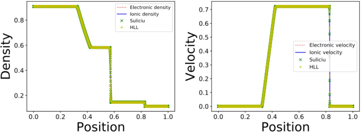
The quantities described by conservative equations (densities and velocities) are consistant with the fluid methods HLL and Suliciu. Moreover, quasi-neutrality is shown to be achieved, since electronic and ionic densities are superposed, as well as electronic and ionic velocities.
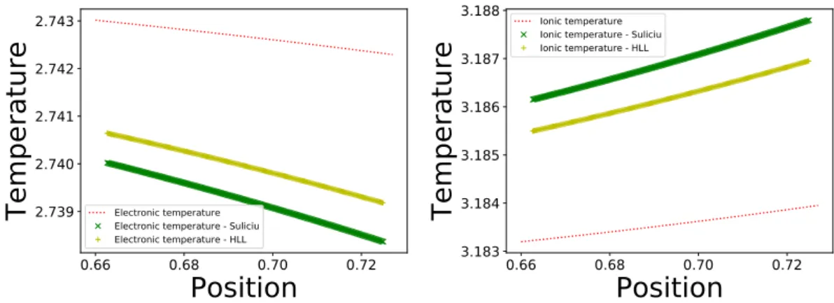
For the partial temperatures presented in figure 2, the intermediate state reached between the rarefaction wave and the contact discontinuity is identical for all schemes, which is expected since this part of the solution is smooth. However, the states obtained between the contact discontinuity and the shock are different for every scheme. Figures 3 display a zoom on this part of the solution. The results can be seen to be different for all three methods. The behaviour of the different schemes should be investigated further.
Shock tube with different initial temperatures. This test case is similar to the previous one, the only difference being the initial left ionic and electronic temperatures. The following initial
Figure 1. Density and velocity solutions of shock tube test case with a mass ratio of 10 with 120000 space points, 40 velocity points and a domain length of 8
Figure 2. Electronic and ionic temperatures of a shock tube test case with a mass ratio of 10 with 120000 space points, 40 velocity points and a domain length of 8 conditions are: I n–(t 0, x) = 1, u–(t 0, x) = 0, T–(t 0, x) = 1 if x œ [0, 0.5], n–(t 0, x) = 0.125, u–(t 0, x) = 0, Te(t 0, x) = 2 Ti(t 0, x) = 3 if x œ [0.5, 1].
Parameters are chosen as Nx = 120000, Nv = 40 and l = 8. The inter-species collision
relaxation time is ·ei = 0.1. Results are computed at time t = 0.1. The result are provided in
figure 4 and 5. The behaviour of the result if very similar to the previous one. Quasi-neutrality is achieved and temperatures exhibit different jump relations across discontinuities for each method. Rarefaction wave. This test case is constituted of two rarefaction waves going in opposite direc-tions. It is given by the following data:
I n–(t 0, x) = 1, u–(t 0, x) = ≠1, T–(t 0, x) = 1 if x œ [0, 0.5], n–(t 0, x) = 1, u–(t 0, x) = 1, T–(t 0, x) = 1 if x œ [0.5, 1].
We have Nx = 120000, Nv = 40 and l = 8. The inter-species collision relaxation time is
Figure 3. Different jump relations through shocks of electronic and ionic tem-peratures for a shock tube test case with a mass ratio of 10 with 120000 space points, 40 velocity points and a domain length of 8
Figure 4. Density and velocity solutions of shock tube test case with a mass ratio of 10 with 120000 space points, 40 velocity points and a domain length of 8
The result are provided in figure 7 and 8. In this test case, the solution is smooth. There are no shock waves, and then, all methods are expected to give the same results. Figure 9 shows that this is what happens.
Shock wave. This test case is constituted of two shock waves. It is given by the following data: I n–(t 0, x) = 1, u–(t 0, x) = 1, T–(t 0, x) = 1 if x œ [0, 0.5], n–(t 0, x) = 1, u–(t 0, x) = ≠1, T–(t 0, x) = 1 if x œ [0.5, 1].
We have Nx = 120000, Nv = 40 and l = 8. The inter-species collision relaxation time is
·ei= 0.1. Results are computed at time t = 0.1.
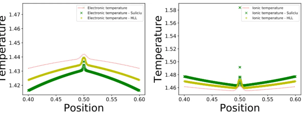
The results are provided in Figure 10 and 11. Quasi-neutrality is achieved on the conserved quantities. The solution contains two shock waves and different jump relations can be observed for each numerical method. In Figure 12, a zoom is performed on the constant values reached by each method between the two shocks. This shows the different behaviour between the three methods.
Figure 5. Electronic and ionic temperatures of a shock tube test case with a mass ratio of 10 with 120000 space points, 40 velocity points and a domain length of 8
Figure 6. Different jump relations of electronic and ionic temperatures for a shock tube test case with a mass ratio of 10 with 120000 space points, 40 velocity points and a domain length of 8
5. Conclusion
In this article, a kinetic numerical method able to provide reference results for a non-conservative hyperbolic system, the bi-temperature Euler system, is proposed. This method is able to enforce all the desired properties that are relevant for comparisons with methods applied directly to the hyperbolic system. Such methods lack an unambiguous definition of the non-conservative prod-ucts and exhibit different Rankine-Hugoniot relation when the solution contains shock waves. However, the proposed method introduces a important amount of numerical viscosity, which ren-ders the method costly. A second-order method able to circumvent such a drawback is a current on-going work, which should be the subject of a subsequent article.
References
[1] R. Abgrall and S. Karni. A comment on the computation of non-conservative products. Journal of Compu-tational Physics, 229(8):2759–2763, 2010.
[2] P. Andries, P. Le Tallec, J.-P. Perlat, and B. Perthame. The Gaussian-BGK model of Boltzmann equation with small Prandtl number. European Journal of Mechanics-B/Fluids, 19(6):813–830, 2000.
Figure 7. Density and velocity solution of a rarefaction wave test case with a mass ratio of 10 with 120000 space points, 40 velocity points and a domain length of 8
Figure 8. Temperature solutions of a rarefaction wave test case with a mass ratio of 10 with 120000 space points, 40 velocity points and a domain length of 8
Figure 9. Zoom on temperature solutions of a rarefaction wave test case with a mass ratio of 10 with 120000 space points, 40 velocity points and a domain length of 8
Figure 10. Density and veloctiy solutions of a shock wave test case with a mass ratio of 10 with 120000 space points, 40 velocity points and a domain length of 8
Figure 11. Electronic and ionic temperature of a shock wave test case with a mass ratio of 10 with 120000 space points, 40 velocity points and a domain length of 8
[3] D. Aregba–Driollet, J. Breil, S. Brull, B. Dubroca, and E. Estibals. Modelling and numerical approximation for the nonconservative bitemperature Euler model. ESAIM: Mathematical Modelling and Numerical Analysis, 52(4):1353–1383, July 2018.
[4] R. Belaouar, N. Crouseilles, P. Degond, and E. Sonnendrücker. An asymptotically stable semi-Lagrangian scheme in the quasi-neutral limit. J. Sci. Comput., 41(3):341–365, 2009.
[5] F. Bouchut. Nonlinear stability of finite volume methods for hyperbolic conservation laws and well-balanced schemes for sources. Birkäuser Verlag, Basel, 2004. OCLC: 928365468.
[6] S. Brull, P. Degond, F. Deluzet, and A. Mouton. Asymptotic-preserving scheme for a bi-fluid Euler-Lorentz model. Kinetic and Related Models, 4(4):991–1023, 2011.
[7] S. Brull, X. Lhebrard, and B. Dubroca. Modelling and entropy satisfying relaxation scheme for the noncon-servative bitemperature Euler system with transverse magnetic field. preprint.
[8] S. Brull and L. Mieussens. Local discrete velocity grids for deterministic rarefied flow simulations. J. Comput. Phys., 266:22–46, 2014.
[9] C. Chalons and F. Coquel. A new comment on the computation of non-conservative products using Roe-type path conservative schemes. J. Comput. Phys., 335:592–604, 2017.
[10] C. Chalons, M. Girardin, and S. Kokh. Large Time Step and Asymptotic Preserving Numerical Schemes for the Gas Dynamics Equations with Source Terms. SIAM Journal on Scientific Computing, 35(6):A2874–A2902, Jan. 2013.
Figure 12. Electronic and ionic temperature of a shock wave test case with a mass ratio of 10 with 120000 space points, 40 velocity points and a domain length of 8
[11] F. Chen. Introduction to Plasma Physics and Controlled Fusion. Number vol. 1 in Introduction to Plasma Physics and Controlled Fusion. Springer, 1984.
[12] F. Coquel and C. Marmignon. Numerical methods for weakly ionized gas. Astrophysics and Space Science, 260(1):15–27, 1998.
[13] P. Crispel, P. Degond, and M.-H. Vignal. An asymptotically stable discretization for the Euler-Poisson system in the quasi-neutral limit. C. R. Math. Acad. Sci. Paris, 341(5):323–328, 2005.
[14] P. Crispel, P. Degond, and M.-H. Vignal. An asymptotic preserving scheme for the two-fluid Euler-Poisson model in the quasineutral limit. J. Comput. Phys., 223(1):208–234, 2007.
[15] G. Dal Maso, P. Le Floch, and F. Murat. Definition and weak stability of nonconservative products. Journal de mathématiques pures et appliquées, 74:483–548, 1995.
[16] P. Degond and F. Deluzet. Asymptotic-preserving methods and multiscale models for plasma physics. J. Comput. Phys., 336:429–457, 2017.
[17] P. Degond, F. Deluzet, and D. Savelief. Numerical approximation of the Euler-Maxwell model in the quasineu-tral limit. J. Comput. Phys., 231(4):1917–1946, 2012.
[18] P. Degond, H. Liu, D. Savelief, and M.-H. Vignal. Numerical approximation of the Euler-Poisson-Boltzmann model in the quasineutral limit. J. Sci. Comput., 51(1):59–86, 2012.
[19] M. Dumbser and D. S. Balsara. A new efficient formulation of the HLLEM Riemann solver for general conservative and non-conservative hyperbolic systems. Journal of Computational Physics, 304:275–319, 2016. [20] S. Guisset, S. Brull, E. D’Humières, and B. Dubroca. Asymptotic-preserving scheme for the M1-Maxwell
system in the quasi-neutral regime. Communications in Computational Physics, 19:301–328, 2016.
[21] S. Jin. Efficient asymptotic-preserving (AP) schemes for some multiscale kinetic equations. SIAM J. Sci. Comput., 21(2):441–454, 1999.
[22] P. G. LeFloch and S. Mishra. Numerical methods with controlled dissipation for small-scale dependent shocks. arXiv:1312.1280 [math], Dec. 2013. arXiv: 1312.1280.
[23] C. Parès. Path-conservative numerical methods for nonconservative hyperbolic systems. In Numerical methods for balance laws, volume 24 of Quad. Mat., pages 67–121. Dept. Math., Seconda Univ. Napoli, Caserta, 2009. [24] K. Xu, X. He, and C. Cai. Multiple temperature kinetic model and gas-kinetic method for hypersonic