Publisher’s version / Version de l'éditeur:
Vous avez des questions? Nous pouvons vous aider. Pour communiquer directement avec un auteur, consultez la première page de la revue dans laquelle son article a été publié afin de trouver ses coordonnées. Si vous n’arrivez pas à les repérer, communiquez avec nous à [email protected].
Questions? Contact the NRC Publications Archive team at
[email protected]. If you wish to email the authors directly, please see the first page of the publication for their contact information.
https://publications-cnrc.canada.ca/fra/droits
L’accès à ce site Web et l’utilisation de son contenu sont assujettis aux conditions présentées dans le site LISEZ CES CONDITIONS ATTENTIVEMENT AVANT D’UTILISER CE SITE WEB.
The Proceedings of the 2007 International Conference onMachine Learning and
Applications (ICMLA '07), 2007
READ THESE TERMS AND CONDITIONS CAREFULLY BEFORE USING THIS WEBSITE. https://nrc-publications.canada.ca/eng/copyright
NRC Publications Archive Record / Notice des Archives des publications du CNRC :
https://nrc-publications.canada.ca/eng/view/object/?id=9a9d977c-faed-4d16-b5aa-c776e6386e2d
https://publications-cnrc.canada.ca/fra/voir/objet/?id=9a9d977c-faed-4d16-b5aa-c776e6386e2d
NRC Publications Archive
Archives des publications du CNRC
This publication could be one of several versions: author’s original, accepted manuscript or the publisher’s version. / La version de cette publication peut être l’une des suivantes : la version prépublication de l’auteur, la version acceptée du manuscrit ou la version de l’éditeur.
Access and use of this website and the material on it are subject to the Terms and Conditions set forth at
Model evaluation for prognostics: estimating cost saving for the end
users
National Research Council Canada Institute for Information Technology Conseil national de recherches Canada Institut de technologie de l'information
Model Evaluation for Prognostics:
Estimating Cost Saving for the End Users *
Yang, C., Létourneau, S.
December 2007
* published in The Proceedings of the 2007 International Conference on Machine Learning and Applications (ICMLA ‘07). Cincinnati, Ohio, USA. December 13-15, 2007. NRC 49867.
Copyright 2007 by
National Research Council of Canada
Permission is granted to quote short excerpts and to reproduce figures and tables from this report, provided that the source of such material is fully acknowledged.
Model Evaluation for Prognostics: Estimating Cost Saving for the End Users
Chunsheng Yang and Sylvain Létourneau
Institute for Information Technology National Research Council Canada
1200 Montreal Road, Ottawa, Ontario K1A 0R6, Canada
{Chunsheng.Yang, Sylvain.letourneau}@nrc.gc.ca
Abstract
Unexpected failures of complex equipment such as trains or aircraft introduce superfluous costs, disrupt operation, have an effect on consumer’s satisfaction, and potentially decrease safety in practice. One of the objectives of Prognostics and Health Management (PHM) systems is to help reduce the number of unexpected failures by continuously monitoring the components of interest and predicting their failures sufficiently in advance to allow for proper planning. In other words, PHM systems may help turn unexpected failures into expected ones. Recent research has demonstrated the usefulness of data mining to help build prognostic models for PHM but also has identified the need for new model evaluation methods that take into account the specificities of prognostic applications. This paper investigates this problem. First, it reviews classical and recent methods to evaluate data mining models and it explains their deficiencies with respect to prognostic applications. The paper then proposes a novel approach that overcomes these deficiencies. This approach integrates the various costs and benefits involved in prognostics to quantify the cost saving expected from a given prognostic model. From the end user’s perspective, the formula is practical as it is easy to understand and requires realistic inputs. The paper illustrates the usefulness of the methods through a real-world case study involving data-mining prognostic models and realistic costs/benefits information. The results show the feasibility of the approach and its applicability to various prognostic applications.
Keywords: Model Evaluation, Data Mining, Machine
Learning, ROC, ROCCH, AUC, Business Gains, Prognostics.
1. Introduction
The need for higher equipment availability and lower maintenance cost is driving the development and integration of prognostic and health management (PHM) systems. Taking advantage of advances in sensor technologies, PHM systems favor a pro-active maintenance strategy by continuously monitoring the health of selected components and warning the
maintenance staff whenever there is a risk for a component failure. These early warnings allow the maintenance staff to devise an optimal repair plan that minimizes both disruption and cost. When sufficient data is available, one may rely on data mining to help build the required predictive models. As an example, we propose in [13] a complete methodology that makes use of classification techniques and existing equipment data to build predictive component failure models. Although this methodology turns out to be highly promising, the problem of model evaluation remains a key practical difficulty limiting the applicability of data mining for prognostics.
Model evaluation is a core topic in data mining and a wealth of approaches and metrics have been proposed. A few examples of traditional approaches include hold-out validation, cross-validation, and bootstrapping. Over the last decade, ROC (Receiver Operating Characteristics) analysis and ROC-based approaches [3, 4, 5 6, 7, 8], including ROCCH (ROC Convex Hull), AUC (Area Under the ROC Curve), and ROC cost curve, have gradually replaced the use of the error-rate measure. The DEA (Data Envelopment Analysis) [9, 10, 11] approach is also gaining popularity in the multi-class problem. Unfortunately, none of these are directly applicable to prognostic applications. There are two reasons. First, these approaches rely on random sampling to select instances during the evaluation process, which is not appropriate whenever there are dependencies between the instances as it is the case in prognostic applications. For example, in prognostic applications one would expect strong dependencies between instances from a given system and between instances with temporal proximity. Ignoring these dependencies during the sampling or the data partitioning process is likely to lead to unrealistic results. Second, these approaches do not take into account the timeliness of the alerts generated by the predictive models and their overall failure detection rate. We proposed a score-based model evaluation approach for prognostics that overcomes some of the limitations discussed above and applied it in various application domains [12, 13]. Although this approach is appropriate for ranking prognostic models, the scores computed do not allow the end user to understand the actual business value of the models built. This paper addresses this
problem by proposing a complementary cost-based method that integrates the various operational costs and benefits involved when making decisions based on prognostic models. From the end user perspective, the formula is practical since it is easy to understand and requires inputs that are usually readily available. The paper illustrates the usefulness of the methods through a real-world case study involving data-mining prognostic models and realistic costs/benefits information.
The following sections of the paper are as follows. Section 2 briefly reviews popular model evaluation approaches for classification tasks and the score-based approach previously proposed for prognostic applications. Section 3 presents the new cost-based model evaluation approach for prognostic applications. Section 4 applies the proposed metric to evaluate data mining-based prognostic models in a real-world application. Section 5 discusses the experimental results, limitations, and future work. Finally, Section 6 concludes the paper.
2. Related Work
In machine learning research, the reliability of a classifier or model is often summarized by either error-rate or accuracy. The error rate is defined as the expected probability of misclassification: the number of classification errors over the total number of test instances. The accuracy is 1 minus the error-rate. Because some errors can be more costly than others, it's sometimes desirable to minimize the misclassification cost rather than the error-rate. For this purpose, several approaches are available, including DEA, ROC analysis, and ROC-based methods. This section briefly reviews these approaches.
2.1 ROC Analysis and ROC-Based Approaches for Model Evaluation
The ROC analysis was initially developed to express the tradeoff between hit rate and false alert rate in signal detection theory [1, 2]. It is now also used to evaluate the performance of classifiers or learning algorithms [3, 4, 5, 6, 7, 8] in machine learning. In particular, ROC is used for performance evaluation of binary classifiers. A binary classifier classifies each instance as “positive” or “negative”. Let us define the true positive (TP) and false positive rates (FP) as follow:
; ; negatives Total classified y incorrectl negatives FP positives Total classified correctly positives TP = =
Using TP and FP as the Y-axis and X-axis respectively, we can plot a ROC space. In this space, each point (FP,
TP) represents a classifier or a model. Given different class distributions and cost-error rates, we plot a curve for a given classifier on the ROC space. This curve is used to determine the performance of a classifier across the entire range of class distributions and error costs. On the other hand, ROC curves alone have limited use for classifier comparison and selection. Several extensions globally referred to as ROC-based analysis have been proposed to address this limitation.
First, let us consider the ROCCH approach [3, 4]. This model selection approach starts by computing a convex hull that encloses the ROC curves for the set of classifiers to be compared. This convex hull represents the best performance that can be achieved from this set of models. Model selection is simply performed by choosing the model(s) that matches the performance of the convex hull for a given class distribution and error cost.
A second approach is the AUC [5, 6, 7], which is more appropriate whenever the class distribution and error cost are unknown. AUC has been shown to be more powerful than accuracy in experimental comparisons of several popular learning algorithms [5]. Precise and objective criteria have also been proposed to demonstrate the superiority of AUC over accuracy [6, 7], in particular with respect to consistency.
A third ROC-based analysis method has been proposed to integrate cost information [8]. This approach relies on cost and normalized cost probability instead of the usual TP and FP rates. Using this approach, the user can assess the expected performance of a model under various costs and event probabilities. Unfortunately, the notion of normalized cost probability, which encapsulates cost and probability information, is often difficult to interpret.
ROC-based approaches are very convenient for the evaluation of models in binary classification tasks but they do not generalize well to multi-class problems. The visualization is specially problematic since the ROC space for a k-class problem has k(k-1) dimensions. And without simultaneous visualization of all the dimensions, the benefits of the ROC approaches are greatly reduced.
2.2 Data Envelopment Analysis
The Data Envelopment Analysis (DEA) method is more effective for multi-class problems. DEA is widely used in decision-making support and management science. It addresses the key issues in determining the efficiencies of various producers or DMUs (Decision Making Units) by converting a set of inputs into a set of outputs [9, 10]. DEA is a linear-programming-based approach, which constructs an efficient frontier (envelopment) over the data and computes each data point’s efficiency related to this frontier. Each data point corresponds to a DMU or a
producer in applications. The task of DEA is to identify the efficiency of the DMUs from the inputs. Z. Zheng, et al. have attempted to apply DEA to model evaluation and combination [11]. They have proved that DEA and ROCCH have the same convex hull for binary classifications. In other words, DEA is equivalent to ROCCH for binary classification tasks. However, DEA can also be used to evaluate models in k-class problems.
2.3 Score-Based Approach for Model Evaluation
The existing ROC-based or DEA-based metrics fail to capture two important aspects for prognostic applications. The first aspect is the timeliness of the predictions. A model that predicts a failure too early leads to non-optimal component use. On the other hand, if the failure prediction is too close to the actual failure then it becomes difficult to optimize the maintenance operation. To take timeliness of the predictions into account, the evaluation method needs to consider the delta time between the prediction of a failure and its actual failure (time-to-failure). The second aspect relates to coverage of potential failures. Because the learned model classifies each report into one of two categories (replace component; do not replace component), a model might generate several alerts before the component is actually replaced. More alerts suggest a higher confidence in the prediction. However, we clearly prefer a model that generates at least one alert for most component failures over one that generates many alerts for just a few failures. That is, the model's coverage is very important to minimizing unexpected failures. Given this, we need an overall scoring metric that considers alert distribution over the various failure cases. We shall now introduce a reward function to take timeliness of predictions into account and then we will present a new scoring metric that addresses the problem detection coverage.
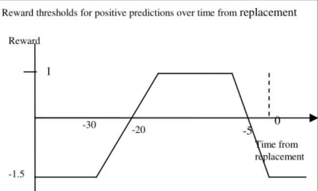
We define a reward function for predicting the correct instance outcome. The reward for predicting a positive instance is based on the number of days between instance generation and the actual failure. Figure 1 shows a graph
of this function. The maximum gain is obtained when the model predicts the failure between five to twenty days prior to a component failure. Outside this target period, predicting a failure can lead to a negative reward threshold, as such a prediction corresponds to a misleading advice. Accordingly, false-positive predictions (predictions of a failure when there is no failure) are penalized by a reward of -1.5 in comparison to a 1.0 reward for true-positive predictions (predictions of failure when there is a failure).
The reward function accounts for time-to-failure prediction for each alert; to evaluate model coverage we must look at alert distribution over the different failure cases. This is taken into account by the following formula to evaluate the overall performance:
where:
• p is the number of positive predictions in the test dataset;
• NbrDetected is the number of failures, which contain at least one alert in the target interval; • NbrofCase is total number of failures in a given
testing dataset; • Sign is the sign of
= p i i sc 1
. When Sign <0 and
NbrDetected=0, score is set to zero; and
• sci is calculated with the reward function above for each alert.
In terms of process, we first adapt the thresholds of the reward function based on the requirements of the prognostic application at hand (rewards, target period for predictions). Then, we run all models developed on the test dataset(s) and compute their score (using Equation 1). The model with the highest score is considered the best model for the application.
3. Evaluating Cost Saving
Although the score-based approach proposed above takes the time-to-failure prediction and problem detection coverage into account for evaluating models, the scores computed do not inform the end users on the expected cost savings of the models. In this section, we propose a new approach that addresses this problem by trying to quantify how much an organization could save by deploying a given prognostic model.
The proposed method is based on the following scenario. The prognostic model is to be implemented in a monitoring system that receives and processes the data
(1) 1 =
= p i i Sign sc NbrofCases NbrDtected Score 1 0
Reward thresholds for positive predictions over time from replacement
Figure 1. A reward function for positive predictions -1.5 Reward -5 -20 -30 Time from replacement
from the equipment in a near real-time manner. Whenever the prognostic model predicts a component failure, an alert is transmitted to the appropriate maintenance staff. After receiving an alert, the maintenance staff will inspect the given component as soon as possible. If the component is found faulty, it would be replaced immediately. Otherwise, the prediction would be considered as a false alert (false positive) and the component will stay in operation.
As with the approach discussed in Section 2.3, the user specifies an optimal target window for the alerts as shown in Figure 2. We use tT and t0 to denote the beginning and then end of this target window. We note that t0also represents the actual failure time. The time at witch the prognostic model predicts a failure (and alert is raised) is noted p. When p <
t
Tthere is a potential for replacing a component before the end of its useful life and therefore losing some component usage. Our approach accounts for this lost of usage by penalizing early alerts proportionally to the difference between p andt
T. By convention, we set t0 =0 and use negative values for times prior to t0 and positive numbers after t0 . Accordingly, we use |p −tT | for the difference betweenp and
t
T. In practice, we use week, day, or hour as time unit.The approach also assumes that the user provides some cost information including the cost of a false alert (an inspection without component replacement), a pro rata cost for early replacement, the cost for fixing a faulty component, and the cost of an undetected failure (i.e., a functional failure during operation without any prior prediction from the prognostic model). The first three costs are generally easy to obtain while the last one is difficult to approximate accurately. This is because failures during operation may incur various other costs that are themselves difficult to estimate. For instance, an operational failure may cause a secondary component to
fail prematurely, it may incur delays in the scheduled operations with potential negative consequences on user’s satisfaction and reputation of the organization, or it may cause a safety hazard and turns into a catastrophe. Although these secondary effects could greatly influence decision regarding the adoption of a prognostic model, the lack of accurate information prevented us from integrating them into the proposed approach. Hence, we adopt a conservative approach and only consider direct costs involved in a functional failure.
To evaluate the cost saving (CS) due to a model, we compute the difference between the cost of operation without the model (Cnm) and the cost with the prognostic
model ( Cpm ). These costs are computed using the following equations: Cnm =c⋅(N+M)+d⋅(M +N) (2) Cpm =a⋅Te+b⋅F+c⋅N+d⋅(M +N) (3) where:
• a is a pro rata cost for early replacement. For example, $10 for each lost day of usage; • b is the cost for a false alert;
• c is the cost for an undetected failure (direct cost for a failure during operation);
• d is the cost for replacing the component (either after a failure or following an alert); • N is the number of undetected failures; • M is the number of detected failures; • Te is the sum of | |
T
t
p − for all predicted failures, i.e., = − = M i T i e p t T 1 | | where pi is the
time of the ith prediction; and • F is the number of false alerts.
As discussed above, the constants a,b,c and d are provided by the end user. Te,F,M and N are computed after applying the given model to an independent testing dataset. The following section presents a real world case study that illustrates the process.
4. A Case Study
The WILDMiner project1 targets the development of data-mining-based models for prognostic of train wheel failures [12]. The objective is to reduce train wheel failures during operation which disrupt operation and could lead
1More information on the WILDMiner project is available at
http://iit-iti.nrc-cnrc.gc.ca/projects-projets/wildminer_e.html time 0 t T
t
Target Alert Failure Alertp
Figure 2, Time relation between alert time and failure time |
to catastrophes such as train derailments. The data used to build the predictive models come from the WILD (Wheel Impact Load Detectors) data acquisition system. This system measures the dynamic impact of each wheel at strategic locations on the rail network. When the measured impact exceeds a pre-determined threshold, the wheels on the corresponding axle are considered faulty. A train with faulty wheels needs to immediately reduce speed and then stop at the nearest siding so that the car with faulty wheels can be decoupled and repaired. A successful prognostic model would be able to predict high impacts ahead of time so that problematic wheels are replaced before they disrupt operation.
For this study, we used WILD data collected over a period of 17 months from a fleet of 804 large cars with 12 axles each. After data pre-processing, we ended up with a dataset containing 2,409,696 instances grouped in 9906 time-series (one time-series for each axle used in operation during the study). We used 6400 time-series for training (roughly the equivalent of the first 11 months) and kept the remaining 3506 time-series for testing (roughly the equivalent of the last 6 months). Since there are only 129 occurrences of wheel failures in the training dataset, we selected the corresponding 129 time-series out of the initial 6400 time-series in the training dataset. We created a relevant dataset for modeling which contains 214364 instances from the selected 129 time-series. Using the obtained dataset and the WEKA package, we built the prognostic models. The model-building process consists of three steps [12,13]. First, we labeled all instances in the dataset by configuring the automated labeling step. Second, we augmented the representation with new features such as the moving average for a key attribute. Finally, we used WEKA’s implementation of decision trees (J48) and naïve Bayes (SimpleNaiveBayes) to build four prognostic models referred to as A, B, C and D. Model A and B were obtained with default parameters from J48 and SimpleNaiveBayes, respectively. In a second experiment, we modified the misclassification costs to compensate for the imbalanced between positive and negative instances and then re-run J48 and SimpleNaiveBayes to generate model C and D.
For evaluation purpose, we ran these four models on the test dataset. The test dataset has 1,609,215 instances. Out of the 3506 time-series contained in the test dataset, 81 comprise a validated wheel failure. We applied the proposed evaluation method to estimate the cost saving from these four models. Since we assumed that the operators will act as soon as they receive an alert (Section 3), we only kept the first alert (prediction of failure) from each time-series. We then extracted the performance parameters N, M, and F by counting the number of time-series for which we did not get any predictions, the number of series for which we did get a prediction followed by an actual failure (true positive), and the
number of time-series for which we got a false alert, respectively. To computeTe, we added the differences
between the time of the prediction and the beginning of the target window (i.e., |p −tT |) for each of the M time-series for which the model correctly predicted a failure. In this application, the time unit for the difference |p −tT | is “day” and tT is set as 20 days prior to failure failure.
For example, when the time-to-failure prediction (p) of an alert is 40 days to an actual failure, its difference,
|
|p −tT , is 20 days (|p −tT |= |-40 – (- 20)| = 20) The cost information (noted a,b,c,and d in Equations (2) and (3)) was provided by an independent expert in the railway industry. These are as follows: a= $2/per day for lost of usage, b=$500/per false alert, c=$5000/per undetected failure and d=$2100/per component replacement. All costs are in US dollars. Using these values and the results for the performance parameters, we obtained the results shown in Table 1.
Table 1, The results of 4 prognostic models on test data.
Model Name T e M+N N F Cost Saving (US$) Model A 357 81 40 245 81,750.0 Model B 812 81 30 178 164,376.0 Model C 647 81 6 161 293,206.0 Model D 1339 81 21 260 167,322.0
5. Discussions and Limitations
The case study illustrates the simplicity and usefulness of the evaluation approach. With this approach, the end user gets a quick understanding of the potential cost savings to be expected from each of the model. Key factors such as timeliness of the alerts and coverage of failures are taken into account, which is not the case with other methods typically used in data mining research. It is worth pointing out that the proposed approach focuses on cost saving and does not tackle the safety issues. It is also interesting to note that, for the case study considered, the results obtained from the proposed method is consistent with the score-based approach described in Section 2.3. It would be interesting to confirm this consistency with additional applications.
The accuracy and applicability of the proposed method is directly linked to the availability and quality of the cost information provided. In the case study
presented, lack of information forced us to adopt a conservative approach by ignoring potential secondary effects of component failures during operation (e.g., cost of derailments, secondary failures, delays in delivery of goods, etc.) Nevertheless, we note from Table 1 that it’s possible to obtain highly positive results even with an overlay conservative approach. Such results could indeed help managers appreciate the values of data-mining-based prognostic models and positively influence their acceptation in real-world applications. We also note that the repair cost is not mandatory in our approach. We could have omitted the corresponding terms in Equations (2) and (3) without changing the results. The other two costs involved: cost for validating an alert and cost due to a false positive prediction should be relatively easy to obtain in many applications.
Finally, it is essential to note that the cost saving analysis proposed fail to capture a number of factors involved in the deployment of prognostic models. For instance, one could assume that there would be some additional costs for the implementation of the model into the existing information system of the organization. Also, accurate prediction of failures may lead to better planning, optimized management of inventory, and increased client satisfaction. All of these improvements would necessarily increase cost saving. Our future work will focus on extending the proposed approach to include such additional factors and therefore improve the precision of the estimated cost saving.
6. Conclusions
In this paper, we first reviewed classical and recent model evaluation methods for classification tasks and then explained their deficiencies for prognostic applications. To overcome these deficiencies, we proposed a cost-based evaluation approach for prognostic models. This novel approach does not only take time-to-failure prediction and problem detection coverage into account, but it also integrates the various costs and benefits information involved in prognostics. From the end user perspective, the formula for computing cost saving is practical as it is easy to understand and requires a minimal amount of information. The experimental results from the case study show that the proposed approach can generate understandable and convincing results that help the end users assess the benefits of prognostic models.
Acknowledgments
Many people at the National Research Council of Canada have contributed to this work. Special thanks go to Bob Orchard, Chris Drummond, George Forester, Jon Preston-Thomas, Richard Liu, David Lareau, and Mike
Krzyzanowski for their support, valuable discussions, and professional suggestions.
References
[1] J. Egan, “Signal Detection Theory and ROC Analysis”, New York Academic Press, 1975
[2] D. Green and J. Swets, “Signal Detection Theory and Psychophysics”, New Your Wiley, 1966
[3] Foster Provost and Tom Fawcett, “Analysis and Visualization of Classifier Performance: Combination under Imprecise Class and Cost Distributions”, Proceedings of International Conference on Knowledge Discovery and Data Mining (KDD1997), 1997
[4] Foster Provost and Tom Fawcett, “Robust Classification for Imprecise Environment”, Machine Learning, 42, pp. 203-231
[5] A.P. Bradley, “The Use of the Area under the ROC Curve in the Evaluation of Machine Learning Algorithms”, Pattern Recognition, Vol. 30, pp. 1145-1159, 1997 [6] Charles X. Ling, Jin Huang, and Harry Zhang, “AUC: a
Statistically Consistent and more Discriminating Measure than Accuracy”, Proceedings of IJCAI 2003, pp. 519-524 [7] Jin Huang, and Charles X. Ling, “Using AUC and
Accuracy in Evaluating Learning Algorithms”, IEEE Transactions on Knowledge and Data Engineering, Vol. 17, NO. 3, March 2005, pp. 299-310
[8] C. Drummond, and R. Holte, “Explicitly Representing Expected Cost: An Alternative to ROC Representation”, Proceedings of the 6th ACM SIGKDD International Conference on Knowledge Discovery and Data Mining (KDD2000), New York, 2000, 198-207
[9] R.D. Banker, A. Chanes and W.W. Cooper, “Some Models for Estimating Technical and Scale Inefficiencies in Data Envelopment Analysis”, Management Science, Vol. 30 No. 9, pp. 1078-1092, 1984
[10] W. Cooper, L. Seiford, and K. Tone, “ Data Envelopment Analysis: A Comprehensive Text with Model, Applications, References, and DEA-solver Software”, Dordrecht, Netherland: Kluwer Academic Publishers, 2002 [11] Z. Zheng, B. Padmanabhan and H. Zheng, “A DEA Approach for Model Combination”, Proceedings of the 10th ACM SIGKDD International Conference on Knowledge Discovery and Data Mining (KDD2004), Seattle, Washington, USA, 2004, 755-758
[12] C. Yang and S. Létourneau, “Learning to Predict Train Wheel Failures”, in Proceedings of the 11th ACM SIGKDD International Conference on Knowledge Discovery and Data Mining (KDD2005), Chicago, USA, August, 2005, 516-525
[13] S. Létourneau, F. Famili, and S. Matwin, “Data Mining for Prediction of Aircraft Component Replacement”, IEEE Intelligent Systems Journal, Special Issue on Data Mining. December 1999. 59-6