HAL Id: hal-01926620
https://hal.archives-ouvertes.fr/hal-01926620v4
Preprint submitted on 7 Jun 2021
HAL is a multi-disciplinary open access
archive for the deposit and dissemination of
sci-entific research documents, whether they are
pub-lished or not. The documents may come from
teaching and research institutions in France or
abroad, or from public or private research centers.
L’archive ouverte pluridisciplinaire HAL, est
destinée au dépôt et à la diffusion de documents
scientifiques de niveau recherche, publiés ou non,
émanant des établissements d’enseignement et de
recherche français ou étrangers, des laboratoires
publics ou privés.
Physically-constrained data-driven inversions to infer
the bed topography beneath glaciers flows. Application
to East Antarctica
Jerome Monnier, Jiamin Zhu
To cite this version:
Jerome Monnier, Jiamin Zhu. Physically-constrained data-driven inversions to infer the bed
topogra-phy beneath glaciers flows. Application to East Antarctica. 2021. �hal-01926620v4�
Noname manuscript No. (will be inserted by the editor)
Physically-constrained data-driven inversions to infer the bed topography beneath
1
glaciers flows. Application to East Antarctica
2
J´erˆome Monnier · Jiamin Zhu 3
4
Received: date / Accepted: date
5
Abstract A method for infering bed topography beneath glaciers from surface measurements (elevation from altimetry 6
and velocity from InSAR) and sparse thickness measurements is developed and evaluated. The method is based on 7
an original non-isothermal Reduced Uncertainty (RU) version of the Shallow Ice Approximation (SIA) equation that 8
natively incorporates the surface measurements. The flow model has a single dimensionless multi-physics parameterg. 9
This parameter takes into account the basal slipperiness and the variable vertical rate factor profiles, thus the vertical 10
thermal variations. The inversions are based on three steps involving: an Artificial Neural Network (ANN) and two 11
Variational Data Assimilation (VDA) processes. The ANN-based stage aims at estimating the multi-physics numberg 12
from the thickness measurements; the resulting estimator is remarkably robust. The full inversion method is valid for 13
half-sheared flows (presenting a moderate basal slipperiness): it can be applied to inland ice-sheets areas. Also these 14
estimates connect continuously with estimates from mass conservation only, i.e. with areas of sliding flows. Numerical 15
results are presented for areas of the East Antarctica Ice Sheet where bed elevation can be very uncertain (Bedmap2 16
values). Estimates are valid for wavelengths longer than ⇠ 10¯h (due to the long wave assumption, shallow flow model) 17
with resolution at ⇠ ¯h (¯h a characteristic thickness value). 18
Keywords Variational data assimilation · reduced flow model · deep learning · inference · topography · glaciers · 19
Antarctica. 20
1 Introduction 21
Bed topography elevation is a necessary input data to set up ice flow models. Also, when combined with surface to-22
pography measurements (e.g. acquired by altimetry), these data directly provide the ice volume. For the Antarctica and 23
Greenland ice-sheets, ice thickness measurements are available along airborne radio-echo sounding tracks e.g. in the 24
CReSIS RDS database1. These measurements are particularly dense in fast flowing areas along the coast. However, the
25
measurements are very sparse or non-existent in the deep land, see [4,14] and references therein. 26
Many satellites have provided (and still provide) accurate measurements of the surface of ice sheets: altimeters provide 27
the surface elevation H at ⇡ ±20 cm for 1 km2pixels see e.g. [22,4], radar interferometers (InSar) provide the surface
28
velocityuHsee e.g. [43].
29
To obtain bed elevation values everywhere beneath the glaciers, the challenge is to infer its value between the thick-30
ness measurement locations, given surface measurements everywhere. A simple method to try to solve this challenge is 31
to apply ordinary Kriging (the interpolation method classically used in geostatistics). This interpolation method can be 32
interpreted as a Gaussian process regression providing the best linear unbiased prediction. This is the method used to 33
obtain bed elevations for Greenland and Antarctica in [3,14]. For the reference Bedmap2 estimates in Antarctica, [14], 34
the authors suggest that for cells within 20km of a measurement, the error is an increasing function of distance. Beyond 35
20 km, the error would be uncorrelated with distance. For cells located more than 50 km from any measurement, the 36
Bedmap2 estimate is based on the gravity field inversion. Therefore, the estimates far from any measurement have very 37
large uncertainties, up to ± ⇠ 1000m according to [14]. 38
To reduce uncertainties in the current bed elevation beneath ice-sheets, combining physically-informed models and 39
J. Monnier
INSA & Institut de Math´ematiques de Toulouse (IMT), France E-mail: [email protected]
J. Zhu
INSA & Institut de Math´ematiques de Toulouse (IMT), France
datasets seems to be the right direction. To do this, a key point is be to employ a flow model that is complex enough 40
to be sufficiently representative but simple enough to lead to stable and well-posed inverse problems (i.e. not leading to 41
severe equifinality issues). In inverse modeling of geophysical flows, equifinality issues are the common pitfall to avoid, 42
see e.g. [5]. 43
44
In fast ice streams (⇡ 1 10 km/y in Antarctica), the flows are plug-like (glaciers slide). In this case, the momentum 45
equation becomes trivial and inverting the (depth-integrated) mass equation allows to fill in the gaps downstream (and 46
upstream) of the measurements, see [46,40]. Because of the nature of the depth-integrated mass equation, measurements 47
(e.g. flight tracks during airborne campaigns) must be acquired cross-lines and relatively dense manner. Indeed, it is well 48
known that this transport equation is intrinsically unstable when inverted, moreover it propagates errors, see e.g. [36] and 49
references therein. To locally blur this feature, one must introduce artificial diffusion which regularizes the equation. The 50
inversion of the mass equation was proposed in [8,46]; then it was combined with surface measurements by Variational 51
Data Assimilation (VDA) in [41,42]. This approach has used to estimate the bed elevation under ice streams, particularly 52
in Greenland [40,42]. 53
In [7], a Bayesian framework is applied to provide probability distributions of the thickness assuming Gaussian covari-54
ance structures of the input data. The algorithm is equivalent to ordinary Kriging if no prior data are available. Bayesian 55
approaches are particularly rich, however, in this case they again relied on mass conservation. 56
For fully sheared flows, the isothermal Shallow Ice Approximation (SIA) flow model with no slip at bottom, was inverted 57
in [37,21]. The obtained estimates are robust but are only relevant for a very restricted flow regime: fully sheared flow 58
areas, thus very slow flows (⇡ 1 10 m/y in Antarctica). 59
In moderately sliding flows, equivalently moderately sheared flows (medium slip, medium shear), the slipperiness at bot-60
tom must be considered in the inversion: it is an additional unknown parameter in addition to the rate factor modeling 61
the internal deformation. Inversions in this flow regime are much more difficult than those in the two regimes described 62
above. The inverse problem is here a-priori ill-posed. 63
Let us cite other studies related to bedrock estimations. [25] inverts the 1D depth-integrated SIA equation with slip and a 64
shape factor that models the 3D characteristics of the flow. This leads to an ill-posed inverse problem, but the inversions 65
are performed by imposing empirical constant values for the unknown parameters. Based on the inversion of the com-66
plete hybrid SIA-SSA system called PISM [55] (SSA for Shallow Shelf Approximation), [51] uses an empirical iterative 67
method to calibrate the bed elevation. In [38], the SIA flow model with slip at bottom is inverted by distinguishing differ-68
ent subregimes. The developed half-analytical half-computational inversion methods lead to well-posed inverse problems 69
and thus stable inversions. The only weakness of the study lies in the ice rate factor which is supposed to be constant. 70
Unfortunately this assumption is not realistic for the Greenland and Antarctica ice-sheets. 71
Inland areas of ice-sheets with medium surface velocities (⇡ [10 100] m/y in Antarctica) correspond to moderately slip-72
ping / moderately sheared flows. These flows cannot be accurately modeled by either mass conservation alone, plug-like 73
flow models (e.g. the SSA model), or fully sheared flow models (e.g. the classical SIA model with no slip at bottom). 74
For these half-slip half-shear flows, the measured surface characteristics (elevation and velocity) are the signature of the 75
bottom slip and internal deformation. Furthermore, the internal deformation depends on the constitutive behavior of the 76
ice and the vertical thermal profiles. Therefore, the inverse problem in this case is very complex. 77
In addition, moderately sheared interior flows have received poorly coverage in airborne campaigns because they are 78
large and distant areas, and therefore to fly over. The flow model to invert must be stable and robust, even in the absence 79
of local in-situ data. This mathematical property is anything but trivial to obtain, see e.g. [2,36,48,38]. In addition, it 80
would be very helpful if the flow model inversion were as insensitive as possible to the measurements locations. 81
Note that an effective bed topography only can be inferred from the surface signature. Indeed, glacier flows act as low-82
pass filters: bed variations are filtered by the flow with filtering characteristics that depend on the flow regime, see [18, 83
34,35] for a detailed discussion. Given a flow regime and a flow model, this then leads to a notion of minimal inferable 84
wavelength, see [19,34,35]. 85
Finally, a comparison of various inverse methods for estimating bed elevation under glaciers (or equivalently ice thick-86
ness) is presented in [12]. The comparison is based on numerous test cases representing a broad spectrum of ice flow 87
regimes. For all test cases, no thickness values are assumed to be known. The 15 methods compared are categorized by 88
type of resolution and not by the range of validity of the method (e.g. based on the flow regime). Numerical comparisons 89
are presented, but no analysis of the equifinality problems present in these inversions is offered. 90
91
The present study aims to solve the following inverse problem: estimating ice thickness (equivalent to bed eleva-92
tion) in half-sheared half-sliding flows with a physically-informed data-driven hybrid method. The targeted flow regimes 93
require consideration fo the full physics of the flows. To do so, a key ingredient is the RU-SIA (RU for Reduced Uncer-94
tainties) model derived in [39]. This flow model is dedicated to the present inverse problem by intrinsically (”natively”) 95
incorporating surface measurements into its coefficients. It is a complete multi-physics flow model, depth-integrated 96
(shallow flow, long-wave assumption). It respects a ”balanced complexity” for its inversion. It takes into account mass 97
conservations and momentum conservation, with a temperature-dependent rate factor: the internal deformation is non-98
uniform, depending in particular on the vertical temperature profiles. In the RU-SIA model, all the complex multi-physics 99
phenomena are consistently represented by a new dimensionless parameter denoted byg. 100
The inversion method developed here is based on a combination of VDA algorithms and a purely data-driven inversion, 101
as in our previous study [39]. However in the one test case studied in [39], a clear correlation existed betweeng and one 102
of the observable fields (|uH|), see [39] Fig. 7. Under these conditions, the estimation of g by a simple Kriging method
103
was possible. However, upon subsequent application of the method to other areas (e.g. those considered in the present 104
study), it was found that no such correlations existed. Therefore, another method to try to estimate this dimensionless 105
multi-physics parameterg had to be investigated. This is what we do here using a Neural Network Residual Kriging 106
(NNRK) algorithm, see [11,30]. Therefore a new inversion method to deduce the bed elevation has been developed; 107
this is the method presented here. The data employed remain the same: surface measurements (elevation, velocity) plus 108
some in-situ thickness values. The inversion method relies on the RU-SIA equation derived in [39], a first advanced VDA 109
process, a deep Artificial Neural Network (ANN) and finally a last VDA process that allows to conclude. The ANN aims 110
to estimate the dimensionless multi-physics parameterg of the RU-SIA model from in-situ ice thickness measurements. 111
These in-situ measurements are available along flight tracks of airborne campaigns. The full inversion method is shown 112
to be mathematically and computationally robust. The areas considered are the East Antartica Ice Sheet (EAIS) regions 113
that a-priori respect the validity domain of the flow model. This corresponds to six large interior regions of EAIS. Recall 114
that it is of interest to accurately estimate the elevation of the EAIS bed because global warming may threaten its stability, 115
particularly around some of the considered areas here, see [13]. 116
In addition a remarkable relationship between current inversions based on the RU-SIA flow model and the widely em-117
ployed mass conservation method, see [46,40,42], is presented. This relationship opens promising prospects for com-118
pleting estimates based on mass conservation alone in deeper regions of ice-sheets. Indeed, we show mathematically that 119
the present and the mass conservation-only estimates meet at the interface of their respective domains of validity, i.e. at 120
the boundaries of plug-like flows (e.g. at and beyond sheared margins). 121
The present inversion method may be applied to all glacier flows as long as the flow model assumption is satisfied i.e. 122
from strongly sheared flows to half-sheared half-sliding flows. Due to the long wave assumption of the flow model, the 123
thickness estimates are valid at a wavelength of ⇡ 10 ⇥ ¯h, ¯h a characteristic thickness value. 124
125
The outline of the article is as follows. In Section 2, the RU equation developed in [38,39] is recalled; its domain 126
of validity is highlighted; the uncertainty of the dimensionless parameterg is analyzed. Then, the inversion method is 127
detailed: Step 1) and Step 3) of the overall algorithm aim at inverting the RU-SIA equation by VDA (physically-informed 128
inversions); Step 2) aims at estimating g using a NNRK algorithm (deep learning, purely data-driven). In Section 4, 129
the six large EAIS areas considered (named Antp, p = 1,..,6) are presented. The methods for obtaining the reference 130
Bedmap2 estimates [14] are briefly recalled. Each computational step of the present inversion method is analyzed in 131
detail. In Section 5, the robustness of the estimations is evaluated in detail for the Ant1 and Ant3 cases, in particular their 132
sensitivities with respect to the presence or not of additional flight tracks. A conclusion is proposed in Section 6. As a 133
complement, the computed thickness estimations for four other areas Antp, p = 2,4,..,6, are presented in Appendix. 134
2 Method 135
In this section the inversion method to estimate the ice thickness h (equivalently the bed topography elevation b) is de-136
tailed. It is done in three steps. Step 1) aims at estimating the product (gh) by assimilating all surface data (altimetry, 137
InSAR and climatic term Source Mass Balance) plus the in-situ thickness measurements in the RU-SIA flow model 138
(model presented below). Step 2) aims at estimating the dimensionless multi-physics parameterg from the in-situ mea-139
surements only (measurements available along the flight tracks of airborne campaigns). Step 3) aims at estimating the 140
thickness h (and adjusting a climatic term) by assimilating all available data again. The final output of the inversion 141
method is the ice thickness h, therefore the bed topography elevation b. 142
143
2.1 The RU-SIA flow model 144
The RU-SIA equation is obtained by reformulating the depth-integrated SIA model with basal slipperiness (see e.g. [17] 145
Chapter 5) but with a non constant rate factor and by natively integrating the surface measurements (elevation and veloc-146
ity). The resulting 2D depth-integrated flow model is original; it is relevant for large scale sheared flows with moderate 147
slipperiness at bottom and with non constant vertical temperature profile. The various uncertain multi-physics param-148
eters (constitutive law exponent, flow regime, temperature dependent term) are gathered into the single dimensionless 149
parameterg. As a consequence, all the physical parametrisation uncertainty is represented by this original dimensionless 150
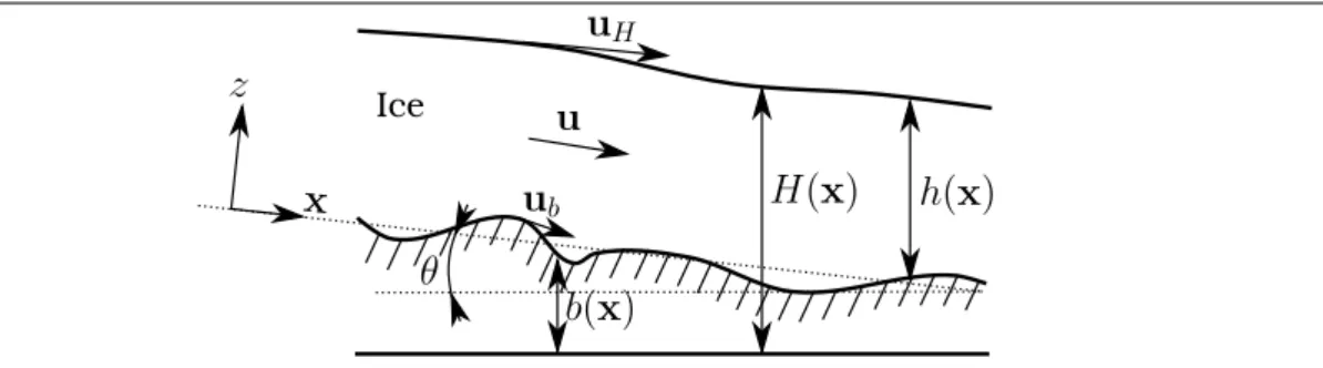
Ice
Fig. 1 Schematic vertical view of the gravitational ice flow and notations
parameter. The basic RU-SIA model assumptions are the same as those for the SIA model (classical lubrication the-151
ory) with basal slipperiness that is: the flow is necessarily sheared (normal stress components are negligible) and it is 152
”shallow” (long wave assumption). 153
2.1.1 The equations and the dimensionless parameterg 154
The surface slope is denoted by S = |—H|; uH is the surface velocity andubis the velocity at bottom (basal velocity).
155
The depth (ice thickness) is denoted by h, h = (H b) with H the ice surface elevation and b the bed elevation, see Fig. 156
1.q is a potential mean slope value in the (x,y)-plane (q = 0 in the forthcoming test areas). 157
158
The flow equation.The depth-integrated flow model SIA model with slipperiness at bottom (see e.g. [17] Chapter 5) is 159
derived in a non isothermal case in [38] providing the so-called xSIA (x for extended) equation. Next in [39], by taking 160
advantage of the measured surface features (elevation and velocity norm), the xSIA model is re-formulated to obtain the 161
RU-SIA model. The RU-SIA equation reads as follows: 162 div ✓ |uH| S gh—H ◆ (x) = ˙a(x) in W (1)
x denotes the space variable and W the considered domain (an open set of R2). The RHS ˙a is the classical one defined
163
by: ˙a(x) = (∂th a)(x) with a the mass balance (accumulation and ablation), see e.g. [17].
164 165
In (1), the term |uH|
S is the observational term; it may provided by InSAR and altimetry surface measurements.
166
The considered unknown of (1) is the surface elevation H. (1) is a linear diffusive equation in H, it is closed by Dirichlet 167
condition at boundaries: H given e.g. by altimetry. 168
Assuming that h (or equivalently b) is given, (1) containsg as the single uncertain parameter. 169
170
The dimensionless parameter.g is the dimensionless parameter of the equation, its expression is, [39]: 171
g(x) =✓1 cA(x)Rs(x) (q + 2)
◆
(2) Rsis the slip ratio describing the flow regime; it is defined as: Rs(x) = 1 |ub|
|uH|(x).
172
The parameter cAis defined by:
173
cA(x) = [(q + 2) (q + 1)RA(x)] (3)
where q is the constitutive power-law exponent (q = 3 in the classical Glen’s law, see e.g. [17] Chapter 5, [38]) and 174
RA(x) =A(x)¯A(x).
175
The parameters ¯A(x) and A(x) are the depth-integrated quantities naturally appearing if the rate factor A depends on 176
(x,z). Their expressions are as follows, see [38]: 177 ¯A(x) =h(q + 2)q+2(x) ✓Z H b Z z b A(x,x)(H(x) x) qdxdz◆ 1 (4) 178 A(x) = (q + 1) hq+1(x) Z H b A(x,z)(H(x) z) qdz (5)
If the vertical profile of A is constant (A constant in z) then: ¯A(x) = A(x) = A(x) 8x. 179
180
Recall that the rate factor A models internal structure properties of the ice. A depends on ice temperature, crystal ori-181
entation, debris content, etc. It may be represented by the Arrhenius law, see e.g. [17] Chapter 4 and references therein. 182
This parameter A highly depends on the temperature, [17], therefore in particular on z in ice sheets. 183
184
Isothermal case.In the isothermal case, A is classically supposed to be a constant, see e.g. [17] Chapter 5. As a conse-185
quence, in this case we obtain: ¯A(x) = A = A(x) 8x. It follows that: RA(x) = 1 = cA(x) 8x.
186
Next for the classically employed value q = 3, it follows:g(x) = 1 1 5Rs(x) .
187 188
2.1.2 Domain of validity of the model 189
The shallowness of the flow is estimated through the geometrical ratioe =H⇤
L⇤, where H⇤and L⇤are characteristic flow
190
depth and length respectively. In these depth-integrated asymptotic models,e has to be small enough, e . 1/10 at least, 191
see e.g. [29]. As a consequence this flow model is valid for a minimal wave length L⇤& 10H⇤. The flow regime is
char-192
acterised by the slip ratio Rs. By construction, the SIA-like models (including xSIA and RU-SIA equations) are valid for
193
Rsranging from ⇡ 0.3 to 1, see [23,47,6] for detailed analysis. This estimation in terms of Rsis numerically quantified
194
in real world cases (including EAIS) in [54]. This study is based on the so-called MCL criteria (criteria proposed in [24] 195
and defined as the length scale over which the terms of driving stress and drag are comparable). In particular it can be 196
noticed that the ice-sheet areas presenting surface velocity ranging in ⇡ [5 100] m/y are accurately modelled by the SIA 197
model as soon as the minimal wave length equals ⇡ 10 12 km in mean. The six test areas Antp considered in the next 198
sections, see Fig. 4, have been defined from the surface velocities norm values: |uH| 2⇡ [10 80] m/y. In these cases
199
H⇤⇡ 2 3 km, then the RU-SIA equation is accurate for minimal wave lengths L⇤⇡ 20 30 km.
200 201
2.1.3 Relationship with the mass equation & its inversion in fast plug-like flows 202
As already mentioned, nice bed elevation estimations are obtained in fast streams by simply inverting the depth-averaged 203
mass equation div(h¯u) = ˙a, ¯u the depth-averaged velocity, see [42]. In [46,41,42], ¯u is related to uH as ¯u = ˜auH, with
204 ˜
a set empirically. In fast streams (actually plug like flows), we have Rs⇠ 0 and ˜a . 1. Therefore, for such cases the
205
uncertainty on the internal deformation (represented in the RU-SIA equation by the parameter cA) is negligible. As a
206
consequence ˜a may be set close to 1 with a few percent error only. This is what is done in these aforementioned studies. 207
In other respect, we can show that: ¯u = |uH|
S g—H, see [39]. Therefore if the slopes S = |—H| and the velocity are
208
co-linear (this is a commonly admitted assumption) than the parameter ˜a empirically defined in [46,41] is nothing else 209
than the dimensionless parameterg defined by (2). 210
This equalityg = ˜a enables building up continuous estimations between fast plug-flows (obtained by inverting the mass 211
equation like in [41,42]) and the moderately sheared / moderately sliding flows (obtained by inverting the present RU-212
SIA equation). 213
On the contrary to plug like flows, in moderately sheared / moderately sliding flows,g varies importantly therefore setting 214
its value empirically is not reasonable anymore. That is why an actual estimation ofg is required. 215
216
2.2 On the uncertainty range of parameterg 217
The dimensionless parameterg defined by (2) depends on various physics parameters: the constitutive law exponent 218
q, the vertical temperature profile through the rate factor A(z) and the flow regime (slip ratio Rs). Recall that the
RU-219
SIA model domain of validity corresponds to Rs2 [⇡ 1./3.,1], see [23,47,6]. For sake of simplicity, q is supposed to
220
be set to the widely employed value for glaciers flows, that is q = 3 (Glen’s law). In isothermal cases, it follows that: 221
g(x) = (1 0.2Rs(x)). Therefore in isothermal cases, the uncertainty on g is relatively small, ⇡ 10% only.
222
The large majority of glaciers are not isothermal in particular those in ice-sheets. Following the Arrhenius law, see e.g. 223
[17, p.54], and by considering typical ice-sheet vertical temperature profiles in ice-sheets, see [44,45] and e.g. [27,49], 224
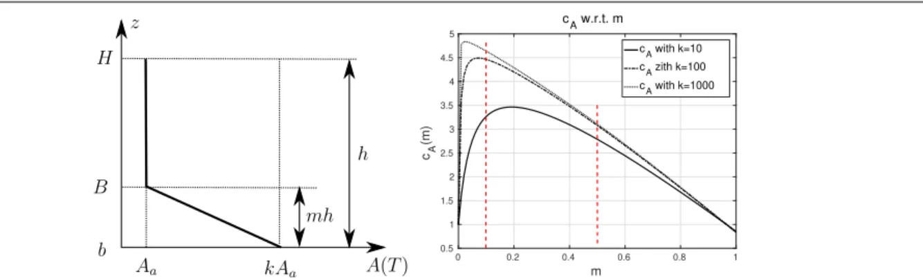
we consider the following vertical profile of A(x,z), Fig. 2 (Left): 225 A(·,z) = ( Aa for z 2 [B(·),H(·)] Aa (B b)(·,z)((1 k)z + kB(·) b(·)) for z 2 [b(·),B(·)] (6)
0 0.2 0.4 0.6 0.8 1 m 0.5 1 1.5 2 2.5 3 3.5 4 4.5 5 cA (m) cA w.r.t. m cA with k=10 cA zith k=100 cA with k=1000
Fig. 2 (Left) A typical vertical profile of rate factor A(·,z), see (6). (Right) The parameter cAvs m, see (3), with k = 10,100 and 1000.
with Aaand k given constants. We define: B(x) = (mh(x) + b(x)) 8x with m 2 [0,1]. Then A(x,z) presents a boundary
226
layer at bottom of thickness (B b)(x) = mh(x), Fig. 2 (Left). The value of cA(x) vs m for different values of k is
pre-227
sented in Fig. 2 (Right). The case m = 0 corresponds to the isothermal case: cA=1. For thin thermal boundary layers cA
228
increases with mh; for thicker layers cAdecreases to a minimal value c(min)A . 1. (This minimal value is reached for the
229
purely linear vertical profile: m = 1). 230
231
Let us consider typical temperature values in EAIS: the bed is at 0C and the surface at 40C . These values 232
correspond to Aa⇡ 10 26therefore k ⇡ 1000, see Fig. 2 (Right). (The value k ⇡ 10 would correspond to typical inland
233
Greenland cases, see [39]). Assuming a boundary layer corresponding to m 2 [0.1,0.5], it follows: cA2 (3.11,4.64) (Fig.
234
2). Finally it follows from (2) that:g(x) ⇡ [1 (0.78±0.15)Rs(x)].
235
This rough uncertainty analysis based on typical values in the targeted areas shows that the uncertainty ong comes 236
similarly from the vertical thermal profile uncertainty (represented by the term (cA/(q + 2))) and the slip ratio Rs. In the
237
targeted regimes and EAIS areas with the vertical profile (6), this corresponds tog varying within the interval ]0,⇡ 0.7]. 238
If relaxing the assumption on the vertical profile as defined in (6), one may estimate the upper bound ofg by setting 239
cA=1 and Rs=0.5 which gives:g 2]0,⇡ 0.9]. (Recall that in fast plug-like flows, g is close to 1).
240
In the forthcoming numerical results, the estimations ofg by the NNRK algorithm are within intervals ]0,⇡ 0.9], see e.g. 241
figs. 6 and 9(Up)(Right). 242
2.3 The inversion method 243
The inversion method to estimate the ice thickness h is developed in three steps. Step 1) and Step 3) are physical-based 244
inversions: the RU-SIA equation (1) is inverted with respect to the product (gh) at Step 1), with respect to (h, ˙a) at Step 245
3). Step 2) is based on an Artificial Neural Network (ANN) aiming at estimatingg; it is a purely data-driven inversion. 246
2.3.1 Sketch of the complete inversion method 247
The estimations of thickness are performed in three steps as follows. 248
Step 1)249 Estimation of the effective diffusivityh = (gh) in RU-SIA equation (1) by VDA. Given the surface measurements (observations) Hobsand |uobs
H |, the effective diffusivity h = (gh) in (1) is infered by
250
solving the following optimal control problem: 251
min
k g(k) with g(k) = gobs(k) + a greg(k) (7)
withk ⌘ h = (gh) and 252 gobs(·) =12 Z W|H(·)(x) H obs(x)|2c tr(x)dx, (8)
ctr is the spatial restriction operator to the flight tracks, greg(·) a Tykhonov’s regularization term, see e.g. [28]. In
253
this step, it is defined as: greg(h) =12RW|—h(x)|2dx. The weight coefficient a is classically set such that it provides
254
a reasonable balance between the physical misfit and the regularization (regularization should be greatly lower than 255
the physical misfit term). The surface elevation H(h) corresponds to the solution of the RU-SIA equation (1) (with 256
Dirichlet boundary conditions) withh given. The gradient of the cost functional is computed by introducing the ad-257
joint equation. The minimisation algorithm is a quasi-Newton method (the L-BFGS algorithm of the Python routine 258
scipy.optimize.minimize).The iterative minimization process is performed until convergence. Numerous numerical 259
experiments have demonstrated robust convergences. In particular the optimal solution does not significantly depend 260
on the smoothing length scale of the surface data (done in the present Ant p test cases at ⇡ 24 km, see next Section), 261
nor on the first guess (set to hbthe Bedmap2 value in EAIS).
262
Past this computational VDA step providing the optimal valueh⇤, the value ofg along the flights tracks where depth
263
measurements hb are available are straightforwardly deduced:gtr⇤ =h ⇤
hbctr(x). These values are inputs of the next
264
algorithm, Step 2). 265
These obtained values are representative at the flow model scale, that is at 10¯h ⇡ 25 km minimal wave length (with 266
⇡ 2km mesh cells), see the investigation presented in [39]. 267
268
Step 2)269 Extension ofg in the whole domain by NNRK. Giveng⇤
tr along the flights tracks (result of Step 1)), a NNRK algorithm ([11,30]) is applied to extend values ofg to
270
the whole area. This statistical learning algorithm is done in two steps: 1) an ANN estimator (deep learning) is built 271
up; 2) an ordinary Kriging of the residuals is added. Details are presented in the next paragraph. 272
273
Step 3)274 Estimation of the pair (h, ˙a) in RU-SIA equation (1) by VDA.
Giveng all over the domain (result of Step 2)), the thickness h is infered simultaneously with the RHS ˙a in (1) by 275
another VDA process. Let us recall them briefly. 276
Similarly to Step 1), the pair (h, ˙a) in (1) is infered by solving the optimal control problem (7) with gobs defined
277
by (8) but minimizing with respect tok = (h, ˙a) (and not w.r.t. h = gh like in Step 1)). In this VDA process, the 278
regularization term reads: 279 greg(h, ˙a) =1 2k(h hb)kCh1+ 1 2k˙a ˙abkCa1 (9) with Ch1and C 1
a covariance operators defining metrics, (hb,˙ab)prior background values (equal to the current
classi-280
cal estimations). The latter are classically defined as the second order auto-regressive correlation matrices with length 281
scale respecting a balance between the regularisation and the preconditioning effects of the VDA algorithm, see [20, 282
39]. Next following [33,20], a change of the control variable is made. The numerous numerical experiments have 283
demonstrated that this choice of covariance operators combined with the change of variable improves greatly the 284
robustness and the convergence speed of the VDA algorithm.In (7) the weight coefficienta is defined as a decreasing 285
sequence following an iterative regularisation strategy, see [28] for an analysis. This iterative regularisation strategy 286
improves the convergence speed of the VDA algorithm too. 287
Numerous assessments of the VDA steps are presented in [39], in particular the sensitivity of the inversions with respect 288
to: i) the uncertainties ong; ii) the density of flights tracks (by removing some of them); iii) the smoothing length scale 289
of the surface data (altimetry, InSar) from ⇡ 24 to 48 km; iv) the first guess (chosen here as the Bedmap 2 value hb).
290 291
Remark 1 Using the explicit expression (2) of g one can compute a-posteriori estimations of the (spatially distributed) 292
slip ratio value Rs. This is an interesting feature to analyse a-posteriori the degree of the RU-SIA flow model consistency.
293
The few a-posteriori analysis made (not presented here) remarkably confirms the good consistency of RU-SIA model. 294
295
Remark 2 Based on a-priori vertical thermal profile(s) (e.g. the one defined by (6)), the RU-SIA equation (1) provides 296
a-posteriori estimations of the effective thermal boundary layer thickness (B b), see Fig. 2 (Left). Such a-posteriori 297
estimations may be interesting for various analyses. Moreover the vertical profiles could be adjusted by constraining 298
them with (the very few) in-situ measurements. 299
2.3.2 Details of Step 2): the Neural Network Residual Kriging (NNRK) algorithm 300
The employed NNRK algorithm is decomposed in three steps as follows. 301
Step 2a)302 Considering the surface data (H, S , |uH|, ˙ab) at all in-situ measurements locations (e.g. along the flights tracks of all
areas Antp) plus the values ofgtr⇤computed at Step 1), an estimator ofg is built up by training a ANN. This estimator
303
is denoted by ¯g. 304
The training dataset is denoted by D; it contains ”examples” (Ii,Oi), i = 1,··· ,Nf t, where Ii= (H,S ,|uH|, ˙ab) (xi)
305
is the i-th input and Oi=gtr⇤(xi)is the corresponding output.xi, i = 1,··· ,Nf t denote the i-th in-situ measurements
306
coordinates (e.g. along the flight tracks). 307
The estimator ¯g is computed as the minimizer of the mean square misfit: 1 Nf tÂ
N f t
i=1(Oi g(I¯ i))2. This misfit function
308
(also called loss function) reads: 309 j(D;·) =N1 f t Nf t
Â
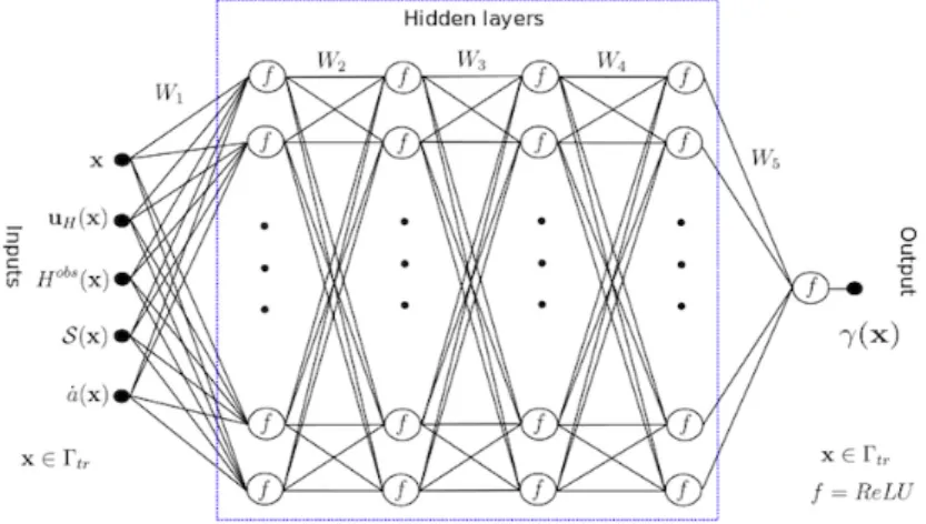
i=1 [g⇤Fig. 3 The Artificial Neural Network (ANN) with four hidden layers. First step of the NNRK algorithm.
To solve this large dimensional data-based optimisation problem, the currently most efficient methods are ANN with 310
few hidden layers (deep learning). Here, 5 layers are considered, see Fig. 3; each of the 4 hidden layers contains 50 311
neurons. The most efficient activation function is chosen: the rectified linear unit (ReLU) function, see e.g. [16,32]. 312
The ANN is determined by its architecture and the weight parameters (W1,··· ,W5), Fig. 3.
313
The training step consists of identifying the optimal values of these parameters Wj, j = 1,..,5. Each Wjis a matrix of
314
dimension nout⇥ nin. Here, W1has 5 ⇥50 = 250 parameters, Wjfor j = 2,3,4 have 50 ⇥50 = 2500 parameters each,
315
W5has 50 ⇥ 1 = 50 parameters. The ANN has been coded in Python using the PyTorch and Mpi4Py libraries [10].
316
To minimize j(D;(W1,··· ,W5))with respect to {Wj}j, the classical Adam method [31], a first-order gradient-based
317
stochastic optimization, is employed. The learning rate (the gradient descent step size) is classically adjusted during 318
the optimization procedure. 319
The input variables are heterogeneous and of different order of magnitude e.g. the elevation H (m) and the slope 320
S (radian). Therefore each input variable v, v an element of {H,S ,|uH|, ˙ab}, are reduced centred as follows:
321
¯vi= (vi mean(v)/s(v)), for all i, 1 i Nf t. The normalisation is applied to mini-batches in hidden layers;
322
this technique is supposed to improve the stability of the model; see e.g. [30] for more details and know-hows on 323
ANN and NNRK algorithms. 324
Also to avoid overfitting, the dropout method [50] is adopted. (This technique may help to prevent overfitting). As 325
usual, the hyper-parameters of the algorithm (learning rate, decay rate, dropout probability) are experimentally cho-326
sen; the selected values are those providing the minimal value of j. 327
328
The ANN has been trained by including hbas an input parameter or not. Both estimators (considering hbas an input
329
or not) turned out to have similar accuracies; thus confirming the strategy to predict the dimensionless parameterg of 330
the flow model from the surface data only. 331
332
Step 2b)333 The K-fold cross-validation method, see e.g. [1], is employed to assess the ANN accuracy and to confirm if the ANN can be used as a predictor. Let us recall that K-fold cross-validation method is as follows, see e.g. [1]:
334
– Divide randomly the original training data set D into K (roughly equal) subsets; 335
– For each subset Dk, k = 1···K, the ANN is trained from the other (K 1) subsets Di, i 6= k.
336
We denote by Ditest= Diand Ditrain=[j6=iDj, i = 1,··· ,K.
337
– Compute the loss function j(Ditest)for each case.
338
Finally, choose the best ANN i.e. those providing the smallest total loss function j(Ditest) +j(Ditrain).
339 340
Step 2c)341 The residual at the measurements locations is computed:eg= (gtr⇤ g) with ¯g computed by the (best) ANN.¯
Next an ordinary Kriging (with a spherical semi-variogram model) is used to extendeg all over the domain. The
342
obtained estimator is denoted by ˆeg. By construction this residual satisfies: E(eg)⇡ 0. Moreover the correlation 343
between two points depends on the distance between them and not on their location. Performing an ordinary Kriging 344
on the residual after ANN is known to be particularly efficient, see e.g. [30] Chapter 3. 345
The final estimator in the whole domain is denoted by ˆg. It is obtained as the sum of the ANN estimator and the 346
ordinary Kriging estimator of residuals: 347
ˆ
The forthcoming numerical results show that the estimator ˆg(x) provides (surprisingly) very accurate values of the 348
parameterg from the surface data only (altimetry, InSAR and ˙a). 349
2.3.3 On the linked uncertainty betweeng and h 350
In the inversion algorithm previously described, after Step 1), one has to separate the effects of the two unknown fields: 351
the physical-based dimensionless parameterg and the ice thicknessh. The accuracy and robustness of each VDA process 352
are demonstrated by the numerical experiments presented later, see also [39]. It will be demonstrated in next section that 353
the NNRK algorithm is robust and accurate too. Then it can be assumed that:gtht⇡ g⇤h⇤; where the superscript ⇤denotes
354
the optimal computed values while the superscript tdenotes the (effective) true value. Let us denote: e
j= (j⇤ jt)/j.
355
At order 1, one has: 356
eh⇡ eg(whereg does not tend to 0) (12)
In other words, Step 2) and Step 3) of the inversion algorithm propagates the error made ong to h in the same order of 357
magnitudes (in %). 358
Remark 3 It would be straightforward to apply the same NNRK algorithm to directly estimate the thickness h all over 359
the domain. However it seems definitively more consistent to estimate a dimensionless parameter of a flow model able 360
to represent accurately the surface data, than to estimate the thickness data partially responsible only of the employed 361
surface data. Following this idea of purely data-driven estimations, [9] had proposed an ANN trained and assessed 362
on synthetic data generated by an ice flow model and geomorphic premises to estimate the bedrock elevation of four 363
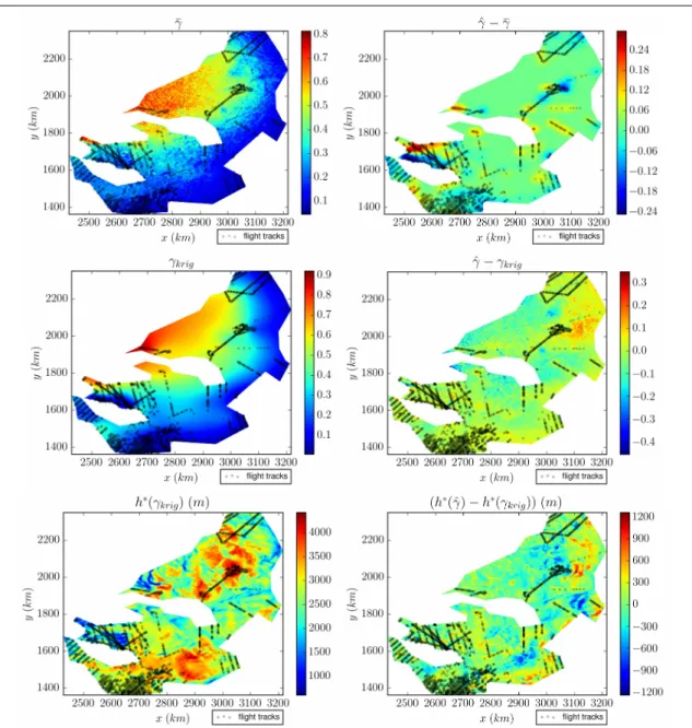
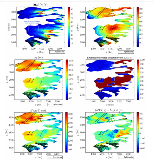
mountain glaciers. 364
3 Data pre-processing 365
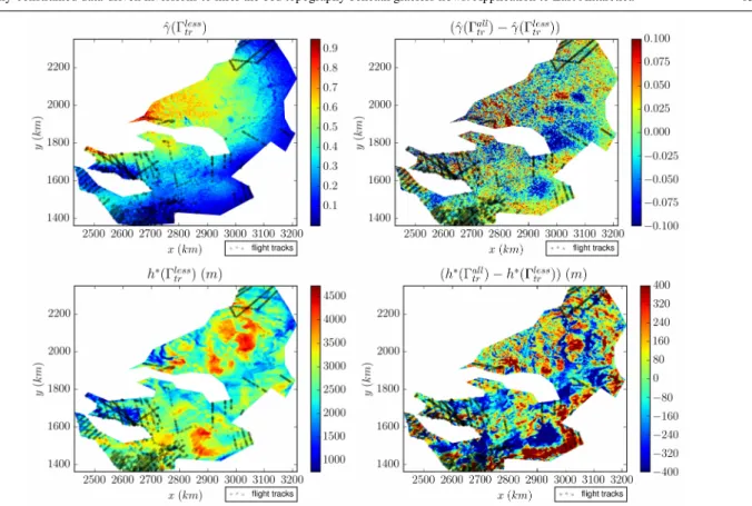
In the next sections, the algorithm is applied to 6 large areas in EAIS (ranging from 250268 to 439045 km2); they are
366
denoted by Antp, p = 1,..,6, see Fig. 4. These areas include the upstream areas of major ice-sheds; all of them respect 367
the flow model domain of validity. The mean thickness value of Bedmap2 ([14]) ranges from 1822 to 2745 m, see tables 368
2-11 for details. The coordinates of the characteristic points defining each area (⇡ 100 150 points per area, see Fig. 4) 369
are available on the open source computational software DassFlow webpage2.
370
Estimating more accurately the bed elevation in these areas may be interesting since global warming may threaten EAIS 371
stability as mentioned e.g. in [13]. 372
373
The correlations between the given variables (Hobs, ku
Hk, S , ˙a, hb) for all areas have been computed. It turns out
374
that no significant linear correlation between the variables have been observed. 375
376
In this section, the method to smooth the surface data accordingly with the flow model domain of validity is presented; 377
the definition of adequate numerical grids follows. Moreover since Bedmap2 values are considered as the reference 378
values, the method to obtain these values is recalled. 379
3.1 Minimal wave length, surface data smoothing and numerical grids 380
The surface data |uH| and H have to be defined at an adequate scale to be consistent with the shallow (long wave
assump-381
tion) flow model (1); next providing a minimal wave length L⇤(km) of the inversions. The RU-SIA equation is accurate
382
as soon ase =[H][L] . 0.1. (In other respect it is shown in [54] that the ice-sheet areas presenting surface velocity ranging 383
in ⇡ [5 100] m/y are accurately modelled by the SIA model as soon as the minimal wave length equals ⇡ 10 12 km 384
in mean). 385
The mean value of the Bedmap2 ice thickness (denoted by ¯hb) [14] in the 6 Antp areas equals ⇡ 2.7 km. In the considered
386
regimes, the velocity field is co-linear to the slopes S ; therefore to be fully consistent, the smoothing of surface data 387
should be done non-isotropically by defining a streamline minimal wave length and a cross-line one. For a sake of sim-388
plicity, here an isotropic smoothing is performed. To do so, a Gaussian with standard deviations = 4 km is convoluted 389
with each given surface field: elevation and velocity norm. Then the smoothing effects are sensitive in disks of diameter 390
⇡ 2 ⇥ (3s) ⇡ 10¯hbkm.
391 392
2 Open-source computational software DassFlow: Data Assimilation for Free Surface Flows. Python version for 2D shallow generalised Newtonian
|u H| (m/y) -2000 -1000 0 1000 2000 eastings (km) -2500 -2000 -1500 -1000 -500 0 500 1000 1500 2000 2500 northings (km) Ocean 0~5 m/y 5~100 m/y >100 m/y 90°W 180° 0° Ant 1 Ant 2 Ant 3 Ant 4 Ant 5 Ant 6 or <5 m/y
Fig. 4 Location of the 6 test areas Antp (east Antarctica) with InSAR-based surface velocity values in m/y (from [43]).
Next a finite element mesh is built up using Gmsh software [15] with a grid sizedx ⇡ 3 km. Indeed dx = 3 km 393
provides ⇡ 10 points per minimal wave length L⇤, therefore respecting the minimal number of points to properly
approx-394
imate all fields. The flight tracks are meshed with cells ofdx ⇡ 2 km. The given thickness measurements (provided in the 395
Bedmap2 database [14]) are interpolated along the flight tracks . 396
397
3.2 Recalls of the origins of Bedmap2 values 398
Bedmap2 values hbare considered as reference values; moreover they are employed to set the first guesses of the VDA
399
processes at Step 1) and Step 3) (see paragraph 2.3.2). hband its a-priori uncertainty as derived in [14] are plotted for each
400
test area Antp in figures 6, 9, 12, 13, 14 and 15 (Middle)(Left). In Bedmap2 database [14], the interpolation - extrapola-401
tion of airborne measurements are performed throughout the domain by the ArcGIS Topogrid routine (ESRI Ltd, ArcGIS 402
9); the latter is based on the ANUDEM algorithm [26]. This algorithm uses an iterative finite difference interpolation 403
technique which is essentially a thin plate spline technique [53]. Next, empirical uncertainty values are stated as follows, 404
see [14]. The thickness measurements are split into two datasets (D1) and (D2). Dataset (D1) is used to build up an inter-405
polation including at Dataset (D2) location points; values of (D2) being not used at this stage. Next, Dataset (D2) is used 406
to quantify the misfit with the ”predicted” - interpolated values; and basic statistics on the results with dependence on the 407
distance to data are deduced. For cells located between 5 and 20km from any data, [14] suggests that the interpolation 408
error is an increasing function of distance from the closest data; beyond it would be not correlated. (Observe that this 409
distance corresponds approximatively to the minimal wave length of the RU-SIA model). For cells that are more than 50 410
km from airborne measurements, the thickness estimation is based on gravity-field inversion (gravity-derived thickness); 411
the proposed related uncertainty equals ±1000m. This is how the uncertainty values on Bedmap2 values hbare defined;
412
see figures 6, 9, 12, 13, 14 and 15 (Middle)(Right). 413
414
4 Analysis of each inversion algorithm step 415
4.1 Step 1: Estimation ofh by VDA 416
The effective diffusivityh defined in (1) is estimated in each area Antp by VDA following Step 1) described in Paragraph 2.3.1. The convergence of this iterative VDA process is very slow (a few hundreds of iterations) but very robust in particular with respect to the first guess value. This step has been thoroughly assessed in [39]. The stopping criteria is the
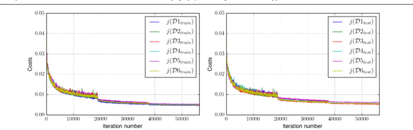
Fig. 5 Misfit functional j(D) defined by (10), vs minimization iterations for: (Left) different train sets Ditrain; (Right) different test sets Ditests. The
learning rate (gradient descent step size) is decayed by 0.2 every 30 epochs (1 epoch = 1 forward pass and 1 backward pass of all the training examples), see e.g. [30] for details on this classical method.
stationarity of khk. Here the RHS ˙a provided by [52] is supposed to be exact. After convergence of the VDA process, given the ice thickness along the flights tracks, the computed optimal valueg⇤is saved for Step 2), that is:
g⇤ tr(x) =h ⇤ hb(x) for x 2 Gtr 4.2 Step 2: Estimation ofg by NNRK 417
The ANN algorithm input values, see Fig. 3, are datasets along all flight tracks in all test areas Antp, p = 1,..,6 plus the 418
values ofg⇤
tr computed at Step 1). This dataset is denoted by D. Following Step 2b) (see paragraph 2.3.2), the K-fold
419
cross-validations are performed with K = 6. The results are presented in Fig. 5. (The value K = 6 is completely indepen-420
dent of the total test cases number). Here, the training sets Ditraincontains 16774 examples and a test set Ditestcontains
421
3354 examples; each example being an (input, output) pair of ANN. 422
It can be read on Fig. 5 (Left) that all ANN models trained from the different data sets Ditrain provide very close cost
423
values j(Ditrain)(see (10)). Moreover, the cost values of all test sets j(Ditest)are almost all equal. This shows that all
424
ANN have very close prediction capability, all being excellent. Indeed after optimisation, j(Ditest)⇡ 5 10 3 (Fig. 5
425
(Right)); this corresponding to ⇡ 1% of the mean value of ¯g. The ANN trained from D2trainis selected since having a
426
slightly smaller misfit value ( j(Ditrain) +j(Ditest)). These tests of prediction capabilities demonstrate the robustness and
427
accuracy of the trained ANN. 428
Next, values of ¯g are predicted in the whole domains Wp, p = 1,··· ,6 by performing the selected ANN.
429
Next by performing the Kriging step (Step 2c) described in Paragraph 2.3.2), the predictor ˆg is obtained. 430
Following the a-priori estimation derived in Section 2.2, the upper bound 0.9 is imposed to the estimation; this upper 431
bound is active at very few locations only; moreover it is in great majority where the uncertainty on hbis low.
432
For each test area, the predicted values ofg are plotted; see figures 6, 9, 12, 13, 14 and 15 (Up) (R). 433
434
4.3 Step 3: Estimation of h (and adjustment of ˙a) by VDA 435
After Step 2), the dimensionless parameterg in RU-SIA equation (1) is given. Then the thickness h is infered by VDA 436
following the method presented in paragraph 2.3.1. The optimisation algorithm converges in ⇠ 20 50 iterations depend-437
ing on the test case. Its convergence is robust; this point has been thoroughly analysed in [39]. 438
At this step, h is simultaneously infered with ˙a. Indeed this enables to adjust the value of ˙a within its uncertainty range 439
which is here ⇠ ±20%, see [52]. It can be noticed in tables 2, 5, 8, 9, 10 and 11 that the corrections made remains in great 440
part within this a-priori uncertainty range. Indeed the upper bound is active at few locations only. In other words, this 441
adjustment based on the physical-based model RU-SIA is consistent with the (totally independent) estimations derived 442
in [52]. 443
Of course, given the surface data, any change of ˙a in RU-SIA equation (1) has an effect on the infered value of h. As an 444
example let us compute the response H of RU-SIA equation (1) in Ant1 area with: i) the RACMO2 value ˙abin the RHS
445
(providing H( ˙ab)); ii) the infered value ˙a⇤by VDA in the RHS (providing H( ˙a⇤)). The obtained difference are the ones
446
indicated in Tab. 1. Therefore the correction made on the RHS ˙a = (∂th a) implies a correction on the ice thickness
447
h negligible (⇠ 1%) compared to the one obtained by the complete inversioin method, see Tab. 2 in next section. This 448
Table 1 Difference between values of H the response of RU-SIA equation (1) if changing the RHS value: ˙abthe Racmo2 value, ˙a⇤the infered value at
Step 3). DomainWp=Ant1.
Difference of H Median Mean Max |H( ˙ab) H( ˙a⇤)| 3.3m 6.0m 26.3m
remark holds for all the domainsWp.
449 450
4.4 On the RU-SIA model accuracy 451
For each test area Antp, domain information and basic statistics on the results are presented, see tables 2, 8, 5, 9, 10, 11. 452
Statistics on the computed surface elevation H, output of RU-SIA model, are indicated. It can be noticed that the RU-SIA 453
equation solved from Bedmap2 value hband the (purely data-driven) estimation ofg obtained at Step 2) already fits very
454
well the measured surface elevation Hobs, see ”Direct model validation” lines in the tables. This very good accuracy
455
(based on the Bedmap2 bed elevation hbi.e. without any additional calibration of h) demonstrates the validity and the
456
relevance of the RU-SIA model. After Step 3) of the inversion algorithm i.e. after the identification of h and ˙a by VDA, 457
of course the RU-SIA model fits even better the measured surface elevation Hobs, see ”|H(h⇤) Hobs| (after h-inversion)”
458
in the tables. 459
460
5 Results and sensitivity tests (Ant1 and Ant3 areas) 461
In this section, the bed elevation b (equivalently the ice thickness h) is infered by the inverse method described in Section 462
2.3 for the two areas Ant1 and Ant3, see Fig. 4, tables 2 and 5. Different estimations of h are compared, depending if: 463
a) isolated flight tracks (hence locally highly constraining) are considered or not; 464
b) the learning method at Step 2) is the NNRK algorithm described in Paragraph 2.3.2, or an ordinary Kriging method 465
like it is done in [39]. 466
These comparisons aim at analysing the robustness and accuracy of the present inverse method. 467
Ant1 is a 370809 km2area north-east upstream of Bailey, Slessor and Recovery ice-streams; Ant3 is a 250268 km2area
468
in Wilhelm and Queen Mary lands, upstream of Shackleton ice shelf and Davis sea. 469
Among the considered six areas, Ant1 and Ant3 are those presenting the largest uncovered parts during airborne cam-470
paigns. As a consequence they contain large areas where Bedmap2 estimation hbis based on gravity field inversions,
471
therefore presenting very large uncertainties. 472
For each case, the domain information and basic statistics on the numerical results are presented in tables 2 and 5. For 473
each case, the most relevant fields are plotted, see figures 6 and 9: the surface velocity norm |uH| and the flight tracks
lo-474
cations (Up)(L), the NNRK estimation ˆg defined by (11) (Up) (R), the Bedmap2 value hb(Middle)(L) with its uncertainty
475
as presented in [14] (Middle)(R), the present thickness estimation h⇤(Down)(L) and its difference with hb(Down)(R).
476
5.1 Results for Ant1 area 477
This domain presents large unexplored areas during the airborne campaigns therefore huge uncertainty on hbvalues, see
478
Fig. 6 (Middle). 479
5.1.1 The ice thickness estimation h⇤
480
Recall that ˆg is the NNRK estimation of the dimensionless parameter g defined by (2).No correlation is observed between 481
h andg; the only clearly observed correlation is : g is small where |uH| is small, see Fig. 6 (Up). This observation is fully
482
consistent with the a-priori analysis done in Section 2.2, see (2) and Fig. 2. 483
Recall that hbvalues are thin plate spline based estimations (see [14] and paragraph 3.1) hence intrinsically smooth, Fig. 6
484
(Middle)(Left). The present estimation h⇤is the optimal solution of a data-driven model combined with a physical-based
485
model; no additional smoothing has been added, then the obtained value h⇤is much less smooth than hb. It is worth to
486
notice that a non isotropic smoothing of the surface data (see the previous section) would have provided bed elevation 487
patterns more correlated to the surface streamlines. 488
The difference between h⇤and hbis not correlated to the distance to the nearest measurement (flight track), on contrary to
489
the empirically stated uncertainty in [14]. Indeed large corrections of hb(up to 1500 m) are obtained close to flight tracks;
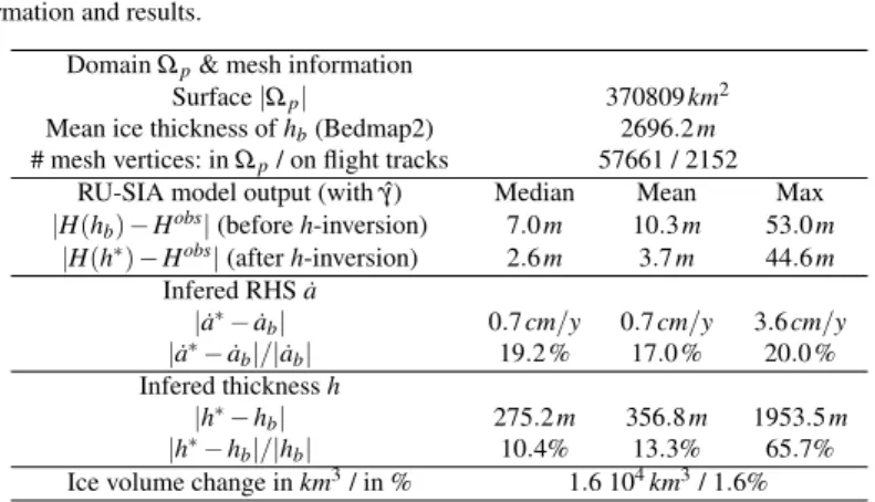
Table 2 Domain Wp=Ant1, information and results.
DomainWp& mesh information
Surface |Wp| 370809km2
Mean ice thickness of hb(Bedmap2) 2696.2m
# mesh vertices: inWp/ on flight tracks 57661 / 2152
RU-SIA model output (with ˆg) Median Mean Max |H(hb) Hobs| (before h-inversion) 7.0m 10.3m 53.0m
|H(h⇤) Hobs| (after h-inversion) 2.6m 3.7m 44.6m
Infered RHS ˙a
| ˙a⇤ ˙ab| 0.7cm/y 0.7cm/y 3.6cm/y
| ˙a⇤ ˙ab|/| ˙ab| 19.2% 17.0% 20.0%
Infered thickness h
|h⇤ hb| 275.2m 356.8m 1953.5m
|h⇤ hb|/|hb| 10.4% 13.3% 65.7%
Ice volume change in km3/ in % 1.6 104km3/ 1.6%
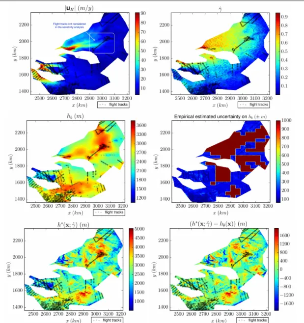
Table 3 Domain Wp=Ant1. Comparison of the estimations if considering or not the flights tracks indicated in Fig.6 (Up)(L).
Infered thickness difference Median Mean Max |h⇤(Gall
tr ) h⇤(Gtrless)| 151.3m 196.9m 1524.5m
|h⇤(Gall
tr ) h⇤(Gtrless)|/|h⇤(Gtrless)| 5.6% 6.6% 80.0%
close meaning at 1 2 minimal wave lengths of the RU-SIA model that is ⇠ 20 40 km, see e.g. in Fig. 6 (Down)(R) the 491
areas around coordinates (2750,1950)(2900,1550)(3050,2050). At the opposite, h⇤may remain very close to hbin areas
492
relatively far from any flight tracks. 493
Recall that the flight tracks are meshed as 1d lines; along these segments (⇡ 2 km long), the infered depth value can 494
vary of ±150m around the measured values (inequality constraints imposed in the VDA processes). Therefore in the 495
adjacent triangles (which are nearly equilateral with ⇡ 2 km edges), the plotted mean depth values may be already much 496
different than the measured ones. This large scale smoothing may explain the potential great differences between the two 497
estimations even relatively close to the flight tracks. 498
The basic statistics presented in Tab. 2 show that after the VDA processes, the RU-SIA equation fits extremely well the 499
measured surface elevation. The correction made on ˙a is relatively consequent, 17% in mean (it is the highest correction 500
made among the 6 test cases Antp). However it remains lower than the maximal authorised correction: ±20%. 501
Finally the correction made on hbis non negligible: 13.3% (356.8 m) in mean, with a 1.6% (1.6 104km3) of volume
502
change only (for 370809 km2).
503
5.1.2 Ant1: if removing some flight tracks 504
In this paragraph, a new ice thickness estimation is computed. It differs from h⇤ since the flight tracks indicated in
505
Fig.6 (Up)(L) are not considered anymore. The original complete set of flight tracks is denoted byGall; the partial one
506
is denoted byGless. InGlesscase, the mesh of the entire area has been re-builded (since in each mesh, the lineaic flight
507
tracks are meshed differently). The inverse problem based onGlessis less constrained in particular the two VDA processes
508
(Steps 1 and 3). Indeed the removed flight tracks are isolated, see Fig. 6(Up)(L); no constraint is imposed in the vicinity 509
of these removed flight tracks anymore. 510
The statistical learning at Step 2) is unchanged, therefore values of ¯g are unchanged too. However the estimation ˆg 511
defined by (11) is not the same since the Kriging step is changed. Indeed the latter is based on less flight tracks data. 512
The difference between the two estimations ( ¯g(Gall) g(Gˆ less))is plotted in Fig. 7 (Up)(R). It can be noticed that ˆg is
513
changed all over the domain and not particularly in the vicinity of the missing flight track. Indeed, the Kriging method 514
(Step 2c) in Paragraph 2.3.2) aims at computing the minimal variance in norm 2 (least square) and not point-wise; hence 515
the global change of ˆg. 516
Next the infered thickness h⇤is different for two reasons: 1) values ofg are different; 2) the VDA process of Step 3)
517
is not locally constrained at the missing flight tracks locations. The difference between the two thickness estimations is 518
plotted in Fig. 7 (Down)(R). For a sake of readability, the legend in Fig. 7(Down)(R) has been bounded at ±400m (very 519
few locations were greater than this bound). Basic statistics on the difference are presented in Tab. 3. Differences of 300 520
m correspond to ⇡ 10 15% of change. As expected, see (12), the variations of h are correlated to the variations of g: 521
compare Fig. 7 (Up)(R) to (Down)(R). Since the global change ofg, the change of h is not particularly important around 522
the missing flight tracks. 523
Finally, it is worth to mention that the present inversion method is relatively global with local constraints (”in-situ” 524
measurements along the flight tracks); it is not purely local inversions. In the present experiment, the obtained variations 525
of h⇤are roughly half of the ones obtained from hb, see tables 2 and 3: difference of 6.6% in mean vs 13.3%, and 5.6%
526
vs 10.4% for median values. 527
Fig. 6 Domain Wp=Ant1 (the plotted coordinates equal the Eastings-Northings plus (2800,2800)km): (Up)(L) Surface velocity module |uH| and flight
tracks (R) ˆg computed by NNRK, see (11). (Middle)(L) Thickness hbfrom Bedmap2 [14] (R) Empirical uncertainty on hbfrom [14]. (Down)(L) Infered
thickness with ˆg: h⇤( ˆg) (R) Difference (h⇤( ˆg) hb).
5.1.3 Ant1: with a different statistical learning method at Step 2) 528
It has been previously shown that uncertainties ong generates uncertainties on h of same order of magnitude, see (12). In 529
this paragraph, the influence of the statistical estimator considered at Step 2) is investigated. To do so, first we compare: 530
a) g obtained by ANN algorithm at Step 2a) to ˆg obtained by the complete NNRK algorithm (see (11);¯ 531
b) gkrigobtained by an ordinary Kriging of values infered along the flights tracks to ˆg.
532
It may be a-priori guessed that a deep learning method (as the present NNRK algorithm) is more reliable than a 533
Kriging inter/extrapolation of its values between the flight tracks. 534
Second, we compare the infered thickness h⇤ obtained from ˆg (that is the original estimation plotted in Fig. 6
535
(Down)(L)) to the one obtained fromgkrig.
536 537
As expected, the difference between ¯g and ˆg (i.e. before and after the Kriging Step 2c) are localised in the vicinity 538
of the flight tracks. In Ant1 case, these differences may be up to ⇠ ±20%, see Fig. 8(Up)(R). More interestingly and as 539
expected too, the differences between ˆg and gkrigare not clearly correlated to the distance to the nearest flight track. The
540
observed difference in Ant1 case may be consequent: ⇠ ±40%, see Fig. 8(Middle)(R). 541
Next, like in the previous sensitivity test (and for the same reasons), the variations of h are correlated to the variations 542
ofg: compare Fig. 8 (Middle)(R) to (Down)(R). Some statistics on the differences are presented in Tab. 4. Again the 543
Fig. 7 Domain Wp=Ant1: comparison if not considering the flights tracks indicated in Fig.6 (Up)(L). (Up)(L) Field ˆg(Gtrless)(i.e. without the flights
tracks indicated in Fig.6 (Up)(L)). (R) Difference ( ˆg(Gall
tr ) g(Gˆ trless)). (Down)(L) Infered thickness h⇤(Gtrless)(R) Difference between the two
estima-tions: (h⇤(Gall
tr ) h⇤(Gtrless)).
Table 4 Domain Wp=Ant1. Comparison the original thickness estimation (obtained using NNRK) to the one obtained using ordinary Kriging at Step2)
Infered thickness difference Median Mean Max |h⇤( ˆg) h⇤(gkrig)| 145.5m 183.5m 1264.2m
|h⇤( ˆg) h⇤(gkrig)|/|h⇤( ˆg)| 5.3% 7.2% 117.2%
obtained variations in h are roughly half of the ones obtained from hb, see tables 2 and 4: difference of 7.2% in mean vs
544
13.3%, and 5.3% vs 10.4% for median values. 545
546
5.2 Results for Ant3 area 547
Like Ant1, Ant3 area presents large uncovered areas during the airborne campaigns, corresponding to huge uncertainty 548
on hb, see Fig. 9.
549
5.2.1 The ice thickness estimation h⇤
550
Like in Ant1 case, the only observed correlation is:g is small if uHis small, see Fig. 9 (Up). Again the difference between
551
h⇤and hbis uncorrelated to the distance to the nearest flight track (on contrary to the empirically established uncertainty
552
in [14]). Large corrections of hb (up to 700 m) are found close to flight tracks see e.g. the area around coordinates
553
(5550,2800) in Fig. 6 (Down)(R); at the opposite, h⇤may remain very close to hbin areas relatively far from any flight
554
tracks, see e.g. the area around coordinates (5250,2800). 555
The few statistics presented in Tab. 5 show that again after the VDA processes, the RU-SIA equation fits extremely 556
well the measured surface elevation. The correction made on ˙a is much lower than the authorised maximal variation: 557
11.2% in mean. In Ant3, the global correction made on hbis relatively low: 6.6% in mean (3.5% median) with a 0.5%
558
of volume change only. However in the most uncertain areas, the corrections made can be either low, see e.g. the areas 559
around coordinates (5000,2650) (5200,3250), or important (± ⇠ 700m), see e.g. the area around coordinates (5000,2650). 560
Fig. 8 Domain Wp=Ant1: comparison between different statistical learning methods at Step 2). (Up)(L) ¯g computed by ANN only. (R) Difference
( ˆg g). (Middle)(L) g¯ krigcomputed by ordinary Kriging. (R) Difference ( ˆg gkrig). (Down)(L) Infered thickness h⇤(gkrig). (R) Difference (h⇤( ˆg)
h⇤(gkrig)).
Table 5 Domain Wp=Ant3, information and results.
DomainWp& mesh information
Surface |Wp| 250268km2
Mean ice thickness of hb(Bedmap2) 1822.8m
# mesh vertices: inWp/ on flight tracks 42881/2443
RU-SIA model output (with ˆg) Median Mean Max |H(hb) Hobs| (before h-inversion) 7.8m 12.7m 274.0m
|H(h⇤) Hobs| (after h-inversion) 2.8m 4.0m 110.6m
Infered RHS ˙a
| ˙a⇤ ˙ab| 2.2cm/y 2.5cm/y 22.1cm/y
| ˙a⇤ ˙ab|/| ˙ab| 11.2% 11.4% 20%
Infered thickness h
|h⇤ hb| 70.0m 124.5m 862.2m
|h⇤ hb|/|hb| 3.5% 6.6% 63.5%
Fig. 9 Domain Wp=Ant3 (the plotted coordinates equal the Eastings-Northings plus (2800,2800)km): (Up)(L) Surface velocity module |uH| and flight
tracks (R) ˆg computed by NNRK, see (11). (Middle)(L) Thickness hbfrom Bedmap2 [14] (R) Empirical uncertainty on hbfrom [14]. (Down)(L) Infered
thickness with ˆg: h⇤( ˆg) (R) Difference (h⇤( ˆg) hb).
Table 6 Domain Wp=Ant3. Comparison if considering or not the flights tracks indicated in Fig.9 (Up)(L).
Infered thickness difference Median Mean Max |h⇤(Gall
tr ) h⇤(Gtrless)| 42.7m 56.3m 904.6m
|h⇤(Gall
tr ) h⇤(Gtrless)|/|h⇤(Gtrless)| 2.2% 2.8% 78.7%
5.2.2 Ant3: if removing some flight tracks 562
The ice thickness obtained if not considering the flight tracks indicated in Fig.9 (Up)(L) is compared to the original 563
estimation h⇤(the one plotted in Fig.9 (Down)(L)). For the same reason as in Ant1 case, both ˆg and h are changed all over
564
the domain and in the vicinity of the missing flight track only. Largest changes are obtained in areas far to the missing 565
tracks; also it may close to (assimilated) flight tracks, see e.g. the area around coordinates (5100,3200). The difference 566
between the two estimations are plotted in Fig. 6 (Up)(R) and (Down)(R). (Again for a sake of readability, the legend 567
in Fig. 10(Down)(R) has been bounded at ±400m; very few values being greater than this bound). Basic statistics on 568
the difference are presented in Tab. 6. (A difference of 200m corresponds to ⇡ 10% of change). Again, the obtained 569
variations on h are roughly half than the ones obtained from hb, see tables 5 and 6: difference of 2.8% in mean vs 6.6%,
570
and 2.2% vs 3.5% for median values. 571
Fig. 10 Domain Wp=Ant3: comparison if not considering the flights tracks indicated in Fig.9 (Up)(L). (Up)(L) Field ˆg(Gtrless)(i.e. without the flights
tracks indicated in Fig.9 (Up)(L)). (R) Difference ( ˆg(Gall
tr ) g(Gˆ trless)). (Down)(L) Infered thickness h⇤(Gtrless). (R) Difference between the two
estima-tions: (h⇤(Gall
tr ) h⇤(Gtrless)).
Table 7 Domain Wp=Ant3. Comparison of the original thickness estimation (obtained using NNRK) to the one obtained using ordinary Kriging at
Step2).
Infered thickness difference Median Mean Max |h⇤( ˆg) h⇤(gkrig)| 58.3m 84.9m 1418.7m
|h⇤( ˆg) h⇤(gkrig)|/|h⇤( ˆg)| 2.9% 4.3% 124.5%
5.2.3 Ant3: with a different statistical learning method at Step 2) 572
Similarly to the Ant1 case, the difference between ¯g and ˆg (i.e. before and after the Kriging Step 2c)) are mainly localised 573
in the vicinity of the flight tracks with amplitudes up to ⇠ ±0.20, Fig. 11 (Up)(R). Again, the differences between ˆg and 574
gkrig are not in the vicinity of the tracks only; they may be anywhere. The observed difference is up to ⇠ ±0.45, see
575
Fig. 11(Middle)(R). Statistics on the differences on the corresponding estimated thicknesses are presented in Tab. 7. The 576
obtained differences on h are about one third lower than the ones obtained from hb, see tables 2 and 7: difference of 4.3%
577
in mean vs 6.6%, and 2.9% vs 3.5% for median values. 578
579
In summary, these empirical sensitivity analyses highlight the robustness and the reliability of the inversion method. 580
If not considering some in-situ measurements (along some flight tracks), see figures 6 and 9 (Up)(L), the obtained differ-581
ences on h are roughly half than the ones obtained between h⇤and hb.
582
If considering a simple Kriging method to estimateg instead of the NNRK algorithm, the obtained differences on h in 583
Ant1 case (resp. in Ant3 case) are roughly 1/2 (resp. 2/3) the ones obtained between h⇤and hb.
584
Therefore in all investigated cases, the obtained variations are lower than the ones obtained from hb, see sections 5.1.1
585
and 5.2.1. 586
6 Conclusion 587
In this study, a method for infering bedrock topography beneath glaciers at a wavelength ⇠ 10¯h (¯h a characteristic 588
thickness value) and with a resolution at ⇠ ¯h, is developed. The key elements of this inversion method are: 1) the Reduced 589
Uncertainty flow model RU-SIA taking into account full physics (including non-uniform internal deformation due in 590
particular to the temperature profile) and presenting a single dimensionless multi-physics parameterg(x); 2) two advanced 591
![Fig. 4 Location of the 6 test areas Antp (east Antarctica) with InSAR-based surface velocity values in m/y (from [43]).](https://thumb-eu.123doks.com/thumbv2/123doknet/14212230.482148/11.892.232.669.115.507/location-areas-antp-antarctica-insar-surface-velocity-values.webp)