Centrifugal compressor return channel shape optimization using adjoint method

Centrifugal Compressor Return Channel Shape

Optimization Using Adjoint Method

INwXSSACHUSETTFS-N

OF TECHNOLOGY

by

NOV 12 2013

Wei Guo

LIBRARIES

B.Eng., Thermal Engineering, Tsinghua University (2011)

Submitted to the Department of Aeronautics and Astronautics

in partial fulfillment of the requirements for the degree of

Master of Science in Aeronautics and Astronautics

at the

MASSACHUSETTS INSTITUTE OF TECHNOLOGY

September 2013

@

Massachusetts Institute of Technology 2013. All rights reserved.

Author

...---

_...

Department of Aeronautics and Astronautics

August 22, 2013

Certified by...

... ...

Qiqi Wang

Assistant Professor of Aeronautics and Astronautics

- j _{Thesis Supervisor}

C ertified by ...

...

Edward M. Greitzer

H. N. Slater Professor of Aeronautics and Astronautics

Thesis Supervisor

Accepted by

(1 .

rofessor

Eytan H. Modiano

of Aeronautics and Astronautics

Chairman, Department Committee on Graduate Theses

Centrifugal Compressor Return Channel Shape Optimization

Using Adjoint Method

by

Wei Guo

Submitted to the Department of Aeronautics and Astronautics on August 22, 2013, in partial fulfillment of the

requirements for the degree of

Master of Science in Aeronautics and Astronautics

Abstract

This thesis describes the construction of an automated gradient-based optimization process using the adjoint method and its application to centrifugal compressor re-turn channel loss reduction. A proper objective function definition and a generalized geometry parametrization and manipulation algorithm were developed, and the ap-propriate adjoint equations and boundary conditions were derived for internal flow of an axisymmetric incompressible laminar flow. The adjoint-based gradient calculation was then validated against finite-difference calculations and embedded in a quasi-Newton optimization algorithm. An optimal design was proposed, which achieved an approximately 5% performance improvement compared to the baseline design in an incompressible laminar flow. The geometry was assessed in a compressible turbulent flow at the actual Mach number and Reynolds number and found to yield a 11% performance improvement for an axisymmetric channel with a previously optimized geometry.

Thesis Supervisor: Qiqi Wang

Title: Assistant Professor of Aeronautics and Astronautics Thesis Supervisor: Edward M. Greitzer

Acknowledgments

First and foremost, I would like to thank my advisors, Professor Qiqi Wang and Pro-fessor Edward Greitzer. I am very grateful to their support and patience throughout my research, without which this thesis would not be possible. Professor Wang has been a constant source of visionary and insightful advice. He not only helped me overcome the steep learning curve of the in-house code, but also encouraged me to see myself as a scientist and look into the root of any research question. Meanwhile, Professor Greitzer has always been a role model for me with his energy, dedication and wisdom. He has taught me countless tips and principles in research and beyond, from which I will surely benefit in future life. It has been a great honor and learning experience working with both tremendous Professors.

This work has been partially supported by the Takasago Research Center of Mit-subishi Heavy Industries. This financial support is gratefully acknowledged.

I am also thankful to my fellow group members, Eric Dow, Patrick Blongian, Han

Chen, Steven Gomez, Rui Chen and Jamin Koo. They never hesitated to give me help and advice on my coursework and research, and I have learned a great deal from each of them. I would like to express my acknowledgment to Anne Aubry and Ben Glass too, whose work has been the foundation of my thesis. I thank them for sharing their knowledge and experience with me selflessly.

Many thanks to my fellow labmates, Tim Palmer, Max Brand, Hadi Kasab and Nikola Baltadjiev, for their help, shared discussions and, of course, shared office space. I will also never forget the sleepless nights preparing for the qualifying exam with Anjaney Kottapalli, Peter Catalfamo and Sebastian Eastham.

This work would not have been the same without my friends, Anthony Pang, Hang Gao, Simon Fang, Shuo Wang, Shuhan Wang, Pei Liu and Zhaoyi Lu. I am deeply indebted to them for their heartily support over my past two years at MIT.

Last but not the least, I would like to sincerely thank my parents. I would not have been who I am without their constant love, support and encouragement.

Contents

1 Introduction

1.1 Background and Motivation . . . .

1.2 Previous Research . . . .

1.3 Research Questions . . . .

1.4 Thesis Contribution . . . . 2 Implementation

2.1 Optimization Framework . . . .

2.2 Objective Function Definition . . .

2.3 Generalized Free-form Deformation

2.4 Adjoint Equation Derivation . . . .

2.5 The Flow and Adjoint Solvers . . .

3 Adjoint Gradient Validation

3.1 Mesh Convergence Study . . . .

3.2 Component-wise Comparisons . . .

4 Assessment of Optimization Result

4.1 Optimal Design for an Axisymmetric Incompressible Laminar Flow

4.2 Design evaluation in an Axisymmetric Compressible Turbulent Flow

5 Summary and Future Work

5.1 Sum m ary . . . . 5.2 Future W ork . . . . 13 13 15 17 17 19 . . . . 19 . . . . 2 1 . . . . 2 3 . . . . 2 6 . . . . 3 4 37 . . . . 3 8 . . . . 4 0 45 45 49 53 53 54

List of Figures

1-1 A horizontally-split MHI centrifugal compressor[9]. Block shows the

return channel... ... 13

1-2 Centrifugal compressor stage schematic [9]. Block shows the return channel ... ... 14

1-3 Locations of baseline geometry separation regions[1] . . . . 15

1-4 Return channel Bezier parametrization[1] . . . . 16

2-1 A typical gradient-based optimization process . . . . 19

2-2 Adjoint-gradient-based optimization process . . . . 20

2-3 Schematic of flow field governing equations and boundary conditions . 21 2-4 FFD example [18]. Left: original geometry, right: deformed geometry 23 2-5 FFD applied to a grid of lines using 4 x 3 control points [18] . . . . . 24

2-6 GFFD mapping schematics . . . . 26

2-7 Gradient results computed using direct finite-difference and residual forcing finite-difference at Re~40 . . . . 28

2-8 Schematic of adjoint field governing equations and boundary conditions 31 2-9 Schematic of adjoint field governing equations and boundary conditions 34 3-1 Effective viscosity field from an axisymmetric compressible turbulent flow calculation in the return channel . . . . 38

3-2 Mesh convergence of the objective function . . . . 39

3-3 Mesh convergence of the residual forcing finite-difference gradient . 39 3-4 Mesh convergence of the adjoint gradient . . . . 40

3-5 Comparison of the adjoint velocity component and the velocity residual

com ponent . . . . 42

3-6 Comparison of the adjoint pressure component and the pressure

resid-ual com ponent . . . . 42

3-7 Comparison of the adjoint gradient and the residual forcing

finite-difference gradient . . . . 43

4-1 Schematics of flow field geometry, governing equations and boundary

conditions . . . . 46

4-2 Optimization convergence history of objective function . . . . 46

4-3 Comparison of baseline design (red) and optimal design (blue) . . . . 47

4-4 Velocity magnitude field of baseline (left) and optimal (right) geometry,

normalized against inlet mean velocity . . . . 48

4-5 Geometry deformation from baseline to optimal design, normalized against inlet width. Left: axial deformation, right: radial deformation 48 4-6 Incompressible laminar flow normalized entropy generation of the

base-line (left) and optimal (middle) geometry, and their difference (right) 49 4-7 Incompressible laminar flow stagnation pressure normalized against

in-let dynamic pressure, of the baseline (left) and optimal (middle) ge-ometry, and their difference (right) . . . . 50

4-8 Compressible turbulent flow normalized velocity field of the baseline (left) and optimal (right) geometry . . . . 51

4-9 Compressible turbulent flow normalized entropy generation of the base-line (left) and optimal geometry (right) . . . . 51

4-10 Compressible turbulent flow stagnation pressure normalized against inlet dynamic pressure, of the baseline (left) and optimal geometry (right) . . . . 52

A-1 Comparison of the adjoint gradient and the residual forcing

A-2 Comparison of the adjoint gradient and the residual forcing

finite-difference gradient . . . . 56 A-3 Optimization convergence history of objective function . . . . 57

Chapter 1

Introduction

1.1

Background and Motivation

Centrifugal compressors are used in gas turbines, automotive engine turbochargers, petrochemical and chemical plants, and many other industries. Centrifugal com-pressors generally have fewer moving parts compared to alternative comcom-pressors, but lower compression ratio in a single stage than reciprocating compressors. As a re-sult, multi-stage centrifugal compressors (shown in Figure 1-1) are widely employed because of relatively higher efficiency than reciprocating compressors.

Figure 1-1: A return channel

horizontally-split MHI centrifugal compressor[9]. Block shows the

As shown in Figure 1-2, a typical multi-stage centrifugal compressor stage consists of an impeller, a diffuser, a 180' return bend, a return vane, and a 90' bend. The last four of these make up the return channel. In all subsequent figures, the return

turn Be d Bladed C Region Shroud Side Shroud ~Side

Entry Hub Bed ExIt

Flaw rz>Side Flow c-:>

Figure 1-2: Centrifugal compressor stage schematic

[9].

Block shows the return chan-nel

channel is displayed in the same orientation as in Figure 1-2, with the left opening as the flow inlet and the right opening the outlet.

Although there is a strong drive to more compact geometries, the change needed can lead to efficiency decrease. Moreover, current compressors have high efficiency, so the return channel design is growing to be a more critical part in overall stage performance.

With fixed inlet and outlet flow conditions, optimizing the return channel design means minimizing the losses through geometry deformation. This is usually realized by tuning a number of geometry design variables. Considering the multi-dimensional nature of such an optimization problem, it is computationally costly to explore the profile design space. Adjoint methods are efficient gradient approximation methods whose computational cost is free from the dimensions of design variables. Adjoint methods have been successfully used in automated aerodynamic design. The emphasis of this thesis is to apply the adjoint method to internal flow optimization and to use it to explore the design space of the return channel in a more comprehensive and automated manner.

1.2

Previous Research

The work in this thesis follows that of Glass [9] and Aubry [1], where important loss mechanisms of the return channel were identified and improved designs were presented.

The principal loss mechanisms included viscous dissipation over the entire channel, and flow separations on the shroud near the bend inlet, on the hub near the bend outlet and due to non-zero incidence angle at the return vane leading edge[9]. Based on quantitative results, the vane section contributes the most to the overall losses. Aubry [1] identified three key locations of flow separations, shown in Figure 1-3 as A, B and C.

Figure 1-3: Locations of baseline geometry separation regions[1]

Based on the loss mechanisms, both Glass [9] and Aubry [1] explored various designs to achieve loss reduction and developed several design guidelines. The pro-posed geometry modifications they explored included a radial diffuser, an increase in the axial extent of return bend, tailored bend width with gradually increasing radius of curvature and a swept back vane channel. The return channel geometry was parametrized and deformed as a series of Bezier patches, as in Figure 1-4. The proposed geometries reduced the computed losses in the return channel, 10% in [9] and 19% in [1], but the optimization was done via trial and error. The design space was thus not explored as fully as it could have been.

Jame-z

Figure 1-4: Return channel Bezier parametrization[1]

son [11, 12]. Instead of evaluating the flow field and calculating the losses repeatedly for every dimension of the geometry design variable that is being modified, adjoint method uses linear approximation to estimate the gradient with respect to all the dimensions in a single run. Jameson [11] borrowed ideas from control theory, and inserted linearized governing equations as controls into the objective function, ap-proximating the gradient without solving the governing equations repeatedly. This proves to be advantageous in reducing the computational cost from proportional to the design variable dimension to only two flow calculations in each optimization iter-ation.

The adjoint method has been successfully used in external flow optimization prob-lems [8, 2, 13], but there are few attempts to apply adjoint method to internal flow optimization problems. Cabuk et al. [4] were among the earliest researchers to do this. They applied the method to optimize a two dimensional diffuser profile for

incompressible laminar flow. Walther et al. [20] employed an adjoint method for a transonic axial compressor stage shape optimization, which is similar to previous external airfoil shape optimization. Relevant attempts on duct flow problems include

[5, 17, 16], which had detailed derivations of adjoint equations and boundary

condi-tions as well as discussion of appropriate objective function selection. However, the form of the adjoint boundary conditions for internal flows was not clear in terms of implementation, and the duct geometries and flow conditions were essentially two dimensional and thus simpler than a centrifugal compressor return channel.

careful setup because improper choices can result in solver divergence or converge to an incorrect solution. This challenge is significant in internal flow problems because the flow field is more sensitive to boundary conditions than in external flow problems where boundaries can be set far away from the flow region of interest. This thesis addresses the numerical instability issues of the boundary condition derivation as well as solution validation.

1.3

Research Questions

In this thesis, an automated optimization process for return channel loss reduction is developed for a simplified subset of internal flow regimes, axisymmetric, incompress-ible, laminar flows. The core of the process, the adjoint method, is derived, validated and applied in the optimization process.

The following research questions are addressed by this thesis are:

" How do we define the optimization problem (objective function and geome-try parametrization) and derive the adjoint equations and boundary conditions for an internal flow problem? What are the differences from an external flow problem?

" How do we validate the results from an adjoint method calculation?

" What is the optimal return bend design determined by the adjoint method, and how much loss reduction can be obtained for an axisymmetric incompressible laminar flow?

" How does a design based on axisymmetric incompressible laminar flow, perform in an axisymmetric compressible turbulent flow?

1.4

Thesis Contribution

* Proper adjoint equations and boundary conditions are derived and validated for the internal flow optimization problem.

" An optimal return channel design is obtained using adjoint method for an

in-compressible laminar flow.

" The loss reduction is assessed in a compressible turbulent flow to provide an

explanatory evaluation of the usability of the incompressible laminar flow situ-ation.

Chapter 2

Implementation

2.1

Optimization Framework

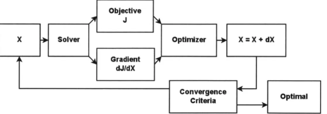
This thesis describes the use of an adjoint method in an automated gradient-based optimization process for return channel design. With reducing losses as the goal and with many continuous design variables to modify, it is reasonable to use a gradient-based optimization method. The optimization process can be illustrated with the flowchart in Figure 2-1. Beginning with a baseline geometry X, each optimization

Objective

X Solver Optirnzer -)o X =X +dX

G nradient dJ/dX

Convergence _Optimnal

Criteria

Figure 2-1: A typical gradient-based optimization process

iteration provides information on the objective function J, a quantitative metric that measures how good the current design is, as well as information on its gradient dJ/dX with respect to the design variables X. Using the gradient information the optimizer then chooses the direction and magnitude of design variable modification dX to effi-ciently proceed with optimization iterations until an optimal design is achieved.

In this thesis, a Quasi-Newton method is employed to utilize the gradient informa-tion to construct an approximainforma-tion of the Hessian matrix, which is a square matrix of all second-order partial derivatives of the objective function. The approximate Hes-sian matrix is then used to provide appropriate direction and magnitude for design variable modification to accelerate the convergence of optimization. The optimizer can be faced with a large number of design variables, resulting in a dense full Hessian matrix and requiring large memory for matrix storage. Therefore, an extension of the

Quasi-Newton method, the limited-memory Broyden-Fletcher-Goldfarb-Shanno

(L-BFGS) method

[3],

is selected to reduce the memory requirement. L-BFGS has been successfully used in aerodynamic design and optimization together with adjoint-based

gradient calculation [7].

Instead of explicitly forming and storing the dense approximate Hessian matrix,

L-BFGS uses history from a few previous steps to update an implicit approximation

of the Hessian matrix at the current step. In this thesis the L-BGFS algorithm from the optimization library NLOpt [14] is used.

The overall optimization process is shown in Figure 2-2. The optimizer starts

Flow Objective Solver J Original Now Geometry LBFGS -oGeometry GFFD X F-X+dX J, aAdjoint Gaintradient Solver dJldX Convergence Optimal Criteria Design

Figure 2-2: Adjoint-gradient-based optimization process

from a baseline geometry X, solves for the flow field to obtain the objective function J, and the adjoint field to obtain the gradients dJ/dX. The optimizer then uses the gradient information to decide what design variable modification dX is needed, and executes the geometry deformation with the geometry deformation algorithm (generalized free-form deformation, GFFD, described in the next section) to form a new geometry X + dX. The optimization loop iterates until the design variable

modification is smaller than a predefined convergence criteria, and the geometry at this step is considered the optimal design. Solving for the adjoint field and calculating the gradient is the central component in the optimization process.

2.2

Objective Function Definition

As a first step in the optimization process, it is necessary to define an object function

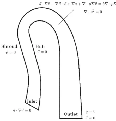
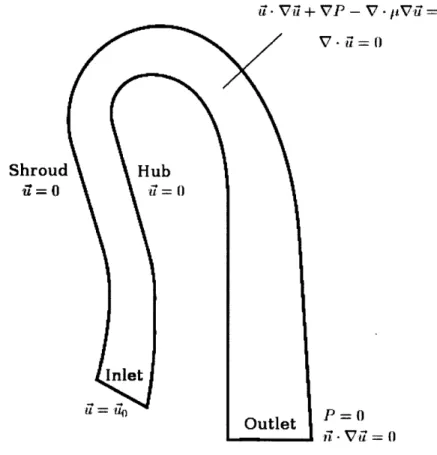
J. Figure 2-3 shows the governing equations and boundary conditions of the flow

field. Hub Inlet Outlet VP - V₁*Vii% V - i=O P=0

Figure 2-3: Schematic of flow field governing equations and boundary conditions

Following previous research [1], an appropriate objective function for a return channel should reflect how much loss is generated in the channel. One definition would thus be the difference in mass flux of stagnation pressure between the outlet

Shroud

and the inlet of the channel. For an incompressible flow,

J-= (nH- pu) P+ p2d A (2.1)

where Q is the flow domain, OQ is the domain boundary, n is the unit normal vector at the boundary, U? is the velocity, p is the fluid density, and P is the static pressure. Equation 2.1 is in terms of a boundary integral. As mentioned in [16] and shown in the later derivation of adjoint equations, using a domain integral instead of a boundary integral as the objective function makes the form of adjoint boundary conditions free from the specific form of the objective function and therefore easier to implement. We thus transform Equation 2.1 to a domain integral.

For a steady incompressible laminar flow, using integration by parts and Navier-Stokes equations, J = j i) )P+ dA (V -j) P + + -) V (P + ))dv -VP+U- _dV2 = ji-(VP+ -V )dV = -(V -pVt) dV j (n-# - pVU) -idA -fV- Vi dV (2.2)

If a velocity inlet, a pressure outlet and non-slip walls are used as the boundary

conditions as shown in Figure 2-3, then we have n -pVu = 0 at the outlet and UT = 0

at the wall. As a result

f,9

(i -pVu) - UdA is zero at these boundaries. We also assume n -pV = 0 at the inlet. If so, we can write

J = (n - pV) -idA - -)VdV 2V3

Since the inlet velocity is enforced in later calculations, A - uVU' is in fact non-zero. However, calculations show only a small difference (-1% in relative difference) be-tween the boundary integral and the domain integral objective functions. This means the gradient-free inlet assumption is a good approximation for an incompressible lam-inar flow using the boundary conditions we have specified.

In this thesis, therefore, we define the objective function as

J = -

j

VU - V'idV (2.4)

the interpretation of which is the entropy generation over the entire flow field.

2.3

Generalized Free-form Deformation

Once the objective function is defined, a geometry parametrization scheme needs to be developed

[1].

The design variables on which the objective function is dependent are defined as the control points derived from the parametrization. In this thesis the free-form deformation (FFD) [19] is used as the basis of the geometry parametrization.

Figure 2-4: FFD example [18]. Left: original geometry, right: deformed geometry

FFD has been widely used in computer graphics, especially computer-aided design,

3D geometric modeling and 3D object sculpturing [19, 10, 6].As illustrated in Figure

2-4, FFD is essentially a map between the original coordinates and the deformed coordinates. The method defines control points aligned as rectangular blocks around the original geometry, and then uses the control points as the basis of Bezier curves to translate the displacement of control points into deformation of the geometry inside

JUF1 -F I I 1U 7u-]-L]

1Xrl 1Z

I r 1M*E1

the blocks. The implementation is that the original geometry is first transformed into non-dimensional coordinates X = Xmin Xmax - Xmin (2.5)

where S is the non-dimensional coordinate, is the original coordinate, Xmin and

Xmax are the coordinates of the corner points of the rectangular blocks. Assuming

(n+

1) x (m+ 1) control points are defined, the deformed non-dimensional coordinates

tare computed as follows

n m

t

z z

b,m(s(1))b,n(s(2))P j

j=0 i=0

(2.6)

where bp,N (u)'s are Berstein coefficients defined as

bp,N(U) N P (1 - N-P,

(P)

p = 0,1,--, N

Here ASj denotes the deformation and wj is a weighting function set as (1, 1) in this thesis. The deformed coordinates are

Xdef = t - (Xmax

-4- .- ..

__ I LI

s=.6

(a) Undeformed Grid with un-displaced control points.

Xmin) + Xmin (2.7)

(b) Deformed Grid.

A key advantage of FFD is its topology-preserving property [18]. As shown in

Figure 2-5, topological relations between the grid lines are preserved after the de-formation, resulting in no lines intersecting with others. This property ensures the quality of the computational mesh to remain stable during deformation, preventing any negative volume cell from being created. FFD also has a disadvantage that the control points for the original geometry have to align in rectangular blocks, and this is very restrictive when deforming a relatively complex geometry such as the return channel. Control points in rectangular blocks cannot provide fine deformation follow-ing the geometry curvature either. Therefore, a generalized FFD (GFFD) has been developed to overcome the control point restriction.

The idea of GFFD is to treat the return channel as the deformed outcome of a rectangle. The inverse mapping function F-1 _{converting the coordinates of the}

rectangle (u, v) into the return channel coordinates (x, y) can be predefined as

(X, y) = F-1 (u, v) = ((X(u), y(U))shroud - (X(U), YC(U))hub) ' V

The forward mapping function F converting the return channel into the rectangle is unknown. Using Newton's method, the map matching the original geometry and the rectangle is solved for and the original coordinates are converted to rectangular coordinates according to the following algorithm:

" Guess rectangular coordinates (U, v)

" Find corresponding guess in original coordinates (x, y) by mapping (x, y)

F-'(u, v)

" Calculate the error E between the (x, y) guess and the true coordinates

" Update rectangular coordinates (U, v) = (u, v) - (VF-')-1 - E

" Loop until the error is small enough (10-12 relative error in this thesis) and

every point is considered matched

Once the rectangular coordinates are found, GFFD follows the conventional FFD and deforms the rectangle. The deformed rectangle is then mapped back into the deformed

return channel. This process is shown in Figure 2-6. The original computation mesh, shown as blue dots in the first subplot is first converted to the rectangle in the second subplot using the forward mapping F. The left boundary of the rectangle is the inlet of the return channel. The FFD control points are assigned to the rectangle, shown as red dots. Going from the second to the third subplot, FFD translates the control point displacement to a deformation of the rectangle. The inverse mapping F-1 is then applied to convert the rectangle back to deformed return channel in the fourth subplot. 00- .- --0-0-- '

L LU.

0. 0 x 0.12 CI4 .Ib i n F ". . 0.4-Forward Mapping -0.2 j.0 Q2 U 0.6 34 * U I FFD I "V 1.0- . . . . .S U.8 n.6 0.04 U F-1 Inverse - -Mapping -x

Figure 2-6: GFFD mapping schematics

2.4

Adjoint Equation Derivation

The next block in the optimization process, the gradient calculation using the adjoint method, is the subject of this section.

Suppose a small perturbation is introduced to the design variables, si, which is

Y

reflected in the objective function J. The conventional way of computing the gradient of the objective function with respect to the design variables, is to use finite-difference (FD)

dJ J(si + si) - J(si)

ds i = 1,2, . I N (2.8)

where N is the dimension of the design variables. This requires N + 1 evaluations of the objective function, or N + 1 flow field solutions. Moreover, a concern about gradient-based optimization methods is that they can only converge to local

opti-mums, and the only way to obtain a global optimum is to start from a number of

different baseline geometries to cover the entire design space, making the problem computationally expensive as the number of flow solutions becomes large. It is this difficulty in high-dimensional gradient-based optimization that motivates the intro-duction of the adjoint method. We therefore use the continuous adjoint method for gradient calculation, as described below.

We can express any small perturbation as having contributions due to a pertur-bation in the flow field and a perturpertur-bation in the geometry.

aJdu

aJ

8

dJ= -ds+ ds=6J+ ds (2.9)

au ds as as

For the perturbed flow field with the unperturbed geometry isi

6J= j (pV- VU-)dV

- 2pV -V'i-dV (2.10)

The original flow field satisfies the following governing equations

V -U = 0 (2.11)

U - VU'+ VP - V - pVG= 0 (2.12)

'In all following discussions, the fluid density p is set to 1 kg/m3 due to the incompressible assumption.

The perturbed flow field satisfies the linearized equations

V -6U = 0 (2.13)

U-V +6 - Vi+V6P -V - P7i= 0 (2.14)

If only the geometry is perturbed and the original flow field is forced to stay

the same, the flow field will not satisfy the linearized equations, and the previous Equations 2.13 and 2.14 become

V -6ui = Rp (2.15)

u -VW+65-Vl+V6P -V1 - Vil= Ru (2.16)

where Rp and RU are non-zero residuals. Rp is denoted as the pressure residual and

RU as the velocity residual.

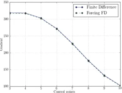
350 .-. Finite Difference - Forcing FD 300 250 200 1150 100 3 8 9 10 Control points

Figure 2-7: Gradient results computed using direct finite-difference and residual forc-ing finite-difference at Re~40

Assume the perturbations made above are small enough that the linear approxi-mations are satisfied. If so, adding the residuals obtained from the unperturbed flow field with the perturbed geometry to the right hand side of the governing equations as forcing terms with the unperturbed geometry should drive the unperturbed flow

field to become the perturbed flow field. To verify this, a test case was run on the return channel to compare the gradient computed using a direct finite-difference and the residual forcing finite-difference. The results are shown in Figure 2-7. 12 con-trol points were put on the return channel shroud, and gradient was computed using the two methods at each control point. Figure 2-7 shows that the gradient results are within 2% for the direct finite-difference and the residual forcing finite-difference. In all following discussions, therefore, the direct finite-difference and residual forcing finite-difference are not distinguished and all gradients, unless specially noted, are computed using residual forcing.

Our next target is to insert the linearized equations as controls into the objec-tive function perturbation in order to eliminate the contribution from the flow field perturbation. This is done by multiplying the linearized equations 2.15 and 2.16 with Lagrangian multipliers, called adj'oint variables in this thesis, V' and q, and plug-ging them into the perturbed objective function. The variable V' is called the adjoint velocity, and q the adjoint pressure.

6J= j(-2pVV -V6u+U - (V -V 6iU-V?7+V6P -V -pV6i)+ (V -5) q) dV

j(.- Ru+q - R)dV

+6P - (V.,U)) dV -j(&W Ru +q Rp)dV

= 0 -p6--+pV--5

To eliminate the contribution from the flow field perturbation, the sum of terms in the domain integration containing 6iU or 6P must be set to zero, forcing the adjoint variables to satisfy the following steady state adjoint equations

V -=0 (2.1_(2.18)

(2.19) l-V - V + V + V -pV= 2V ,pV

The terms in the boundary integrals must be eliminated also, yielding

6U- (2n'- pV+n' - V + ( - )+ q -n)

+6P

.- * .- - (-- - PV6 -' + 2 1) = 0 (2.20)

This results in the following adjoint boundary conditions:

9 At the inlet and wall, since the velocity stays the same, 6u = 0, and the shear

stress is assumed negligible, meaning ' - VU ~ 0, we have

6P - n - v = 0 (2.21)

o The outlet is set as a pressure outlet, so 6P = 0, and ' - V7' = 0. Thus

(2.22)

The form of adjoint boundary conditions implemented are

" At the inlet and wall

" At the outlet

V= 0 (2.23)

T= 0, q = 0 (2.24)

The adjoint field reflects how much an upstream perturbation can influence the downstream flow field, which means the adjoint field generally propagates in the

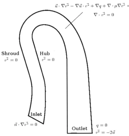
VJ* V- VdZ - - Vq + ud Hub 00 Inlet Outlet 1itZVJV

Figure 2-8: Schematic of adjoint field governing equations and boundary conditions

opposite direction of the flow field. The inlet of a flow field thus serves as an "outlet" in the adjoint calculation and usually has little influence over the adjoint field upstream if set correctly. In the return channel calculation, setting the inlet adjoint boundary with a Dirichlet boundary condition turns out to cause reflections and numerical oscillations near the inlet. To damp out the oscillation, an artificial viscosity nine times the laminar viscosity is introduced to the domain from the inlet to one inlet width downstream. The inlet is set as an outflow Neumann boundary so that the remaining oscillations are carried outside the channel. The final form of the adjoint boundary conditions are

o At the inlet

n - Vi'= 0 (2.25)

* At the wall

v= 0 (2.26)

e At the outlet

&= 0, q = 0 (2.27)

The overall adjoint field schematic is shown in Figure 2-8. The artificial viscosity layer is excluded from the objective function integration domain. The influence on loss reduction and gradient calculation is negligible because the layer is very thin and the inlet geometry and velocity remain unchanged.

The only terms left in the perturbed objective function are the domain integrals containing the residuals, and the gradient can be calculated as

dJ V-=--1 __ (.28

("-,- Ru + q- Rp)dV + ai(2.28)

ds ds ]V

VPas

+

The adjoint equations 2.18 and 2.19 have also been seen in [4, 17, 22]. However, [4] and [17] both mentioned that some adjoint equation formulations may cause insta-bility in solutions, though no definitive fix was derived. Looking back on the adjoint equations

V -V, = 0 (2.18)

U - V #- V -U+ Vq + V - pVV= 2V [ pVi (2.19)

and the adjoint boundary conditions * At the inlet n -V& = 0 (2.29) " At the wall V= 0 (2.30) " At the outlet J = 0, q = 0 (2.31)

it can be noticed that no adjoint velocity or pressure goes into the domain from the boundaries, so the only force driving the adjoint field is the right hand side of the adjoint momentum equation, 2V - tV. As the laminar viscosity p becomes smaller, the forcing will become too small to distinguish from numerical oscillations. Based on this assumption, the adjoint equations are reformulated.

Start by substituting (' - 2M) with v

V - V + V - =0 (2.32)

- V u v+ - V + V -V = 0 (2.33)

Since U' satisfies the continuity equation, we have

V -V = 0 (2.34)

u - Vz- Vu- i + Vq + V - pV[ = 0 (2.35)

And the adjoint boundary conditions become the following form accordingly

" At the inlet n - VV = 0 (2.36) " At the wall V = 0 (2.37) * At the outlet = -25, q = 0 (2.38)

In the new formulation the adjoint field is driven not by a forcing term but instead

by the adjoint velocity entering the channel outlet with the magnitude of 2u. The

overall adjoint field schematics are shown in Figure 2-9. Using the new formulation, a set of new adjoint gradient results are obtained as

dJ _1 - 8

-=-- ((V* + 2)-Ru +q-R)dV+ (2.39)

ud Hub Inlet Outlet *Vq + V - -~i, 0 V. 0 q=0 - -i

Figure 2-9: Schematic of adjoint field governing equations and boundary conditions

The adjoint field V* and q is independent of the design variables S. RU, Rp and 9

are evaluated for each dimension of the design variables, but the computational cost is trivial. Therefore, all gradients can be obtained at the cost of one flow solution and one adjoint solution.

2.5

The Flow and Adjoint Solvers

The implementation of adjoint method requires in-depth knowledge of the flow solver. For this reason, commercial CFD softwares were not used for this thesis and in-house codes were developed and employed.

The flow solver used solves the continuity equation and unsteady Navier-Stokes equations. The adjoint solver solves the unsteady version of the adjoint equations derived in the previous section. The unsteady simulation is run until it reaches a

Shro

steady state, determined by tolerances set for the flow field and adjoint field variation during each time step. The numerical scheme in the solvers, which is almost identical to that used in the code CDP [15] developed at Stanford University, uses second order discretization in space and time. Details of the numerical scheme can be found in

Chapter 3

Adjoint Gradient Validation

In this thesis we use an axisymmetric incompressible laminar flow calculation as a simplified scenario for the return channel optimization problem. A velocity inlet with parabolic velocity profile is selected to reduce the loss from viscous dissipation near the inlet. In contrast, a uniform inlet velocity profile with the same mean yields nearly three times the loss in the flow field. A pressure outlet and non-slip walls are also used as the boundary conditions for the flow field.

The laminar viscosity is set to the cell volume average effective viscosity based on a compressible turbulent flow return channel calculation in ANSYS Fluent to provide some connection to the actual situation. The effective viscosity field is shown in Figure 3-1. The cell volume average effective viscosity is approximately 0.01 and the inlet Reynolds number in the following calculations are therefore approximately 400. The relevance of the solution obtained using the simplifications will be discussed in the next chapter. This chapter focuses on validating the gradient results using an adjoint calculation against gradients obtained by finite-difference calculation.

Axisymmetric test cases were first run at low Reynolds numbers (Rem4 and Re-40). The adjoint gradients agree well with finite-difference gradients at those low Re, and the detailed comparison is covered in the Appendix. The discussions in this chapter covers the calculation at Re-400. 12 control points were evenly put along the shroud, with another 12 control points along the hub. The nearest two control points to the inlet and the outlet were frozen to ensured fixed inlet and outlet

Effective Viscosity 0.02 0.019 0.018 0.017 0.016 0.3 0.015 0014 0.013 0.012 0.011 0.01 0.009 0.008 0.25 0.007 0.006 0.005 0.004 0.003 0.002 0.001 0.2 0.1 0.15 0.2

x

Figure 3-1: Effective viscosity field from an axisymmetric compressible turbulent flow calculation in the return channel

geometry. Since numerically the roles of hub and shroud are the same in the flow and adjoint calculations, only the gradient calculations for shroud control points are shown.

3.1

Mesh Convergence Study

A mesh convergence study was first carried out to determine if the mesh was

suffi-ciently refined for flow field and adjoint field calculations. Three mesh files, denoted as "regular mesh", "fine mesh" and "finer mesh", have 35136, 70272 and 140544 nodes in the 2D domain respectively. The objective functions, finite-difference gradients and adjoint gradients computed on all three mesh files are shown in Figures 3-2, 3-3 and 3-4. Both the objective function (< 1% change) and gradients (< 3% change) have marginal change as the mesh is refined, implying the flow field and adjoint field cal-culation have achieved mesh convergence. Later calcal-culations use the "regular mesh"

Objective function mesh convergence

1.0

Regular -+ fine -+ finer uiesh

Figure 3-2: Mesh convergence of the objective function

FD gradient mesh convergence

--- - -~-1 - A h -h

w- -e Forcing, finer mesh 9. -- Forcing fine mesh

9- -e Forcing regular mesh

4 5 6 7

Control points

8 9 1J

Figure 3-3: Mesh convergence of the residual forcing finite-difference gradient 95.40 95.35 95.30 95.25 95.20 95.15 0 95.10 95.05 0.5 1.5 2.0 -4 -6 -8 -10 -12 -14 -16 -18

-4 -6 -12 -_14 -16 -18

Adjoint gradient mesh convergence

-

-

---eAdjoint, finer mesh

- Adjoint fine mesh

- Adjoint. regular mesh

Control points

8 9 10

Figure 3-4: Mesh convergence of the adjoint gradient

3.2

Component-wise Comparisons

From Equation 2.39, the adjoint gradient can be expressed as

dJ _1

-V

--ds ds L((V* + 2) - Ru + q - R)dV +

aJ

as (2.39)

The adjoint gradient consists of three components, the adjoint velocity component

(V* + 2i) -RudV ds " - _{1q - RpdV} ds fo (3.1) (3.2) (3.3) as

In the residual forcing finite-difference calculation, the gradient is also made up of three different components. The first is the velocity residual component, which is the gradient computed when the residual forcing is applied to the Navier-Stokes the adjoint pressure component

equations on an unperturbed geometry

V =0 (3.4)

S- Vul+ VP - V -pVU= Ru (3.5)

The second component is the pressure residual component, which is the gradient com-puted when residual forcing is applied to the continuity equation on an unperturbed geometry

V - '= RP (3.6)

U - Vi+ VP - V - PVU= 0 (3.7)

The third component is the geometry component, which is computed using the origi-nal converged flow field and the perturbed geometry. The geometry component here is the same as in the adjoint gradient.

Figure 3-5 shows the comparison of the adjoint velocity component and the ve-locity residual component, Figure 3-6 shows the comparison of the adjoint pressure component and the pressure residual component, and Figure 3-7 shows the compari-son of the adjoint gradient and the finite-difference gradient. The three figures show that even though the relative error at some points can be as large as 40% between the adjoint gradient and the finite-difference gradient, they have the same signs and trend with respect to control points. Therefore, the adjoint gradients are taken as validated and useful to apply in the optimization process.

Momentum eqn forcing only

. - Residual U Forcing

s--e Adjoint U component

6p t

Control points 8 9

i10

Figure 3-5: Comparison of the adjoint velocity component and the velocity residual component

Continuity eqn forcing only

.- Residual P forcing . -e Adjoint P component -U 5 6 -Control points 8 9 WU

Figure 3-6: Comparison of the adjoint pressure component and the pressure residual component 20 10 0 -10 -20 -30 -40 50 40 30 20 10 Q -10

5 6 7 Control points

8 9 10

Figure 3-7: Comparison of the difference gradient

adjoint gradient and the residual forcing finite--41

-6

-10

-12

.14

FD gradient vs. adjoint gradient

D-. Fd -eAdjoint

-16 _-18

Chapter 4

Assessment of Optimization Result

4.1

Optimal Design for an Axisymmetric

Incom-pressible Laminar Flow

Using the components described in Chapters 2 and 3, an optimization case of an axisymmetric return channel is performed at Re~~400 starting from the baseline ge-ometry shown in Figure 4-1 which is the optimized gege-ometry from [1].

A total of 12 control points were on the shroud and another 12 on the hub. The

number of control points is a balance between the degrees of freedom for the geometry deformation and the rate of convergence of the optimization. The two control points on both the shroud and the hub nearest to the inlet and the outlet were frozen to fix the inlet and outlet geometry. The actual optimization problem is thus 16 dimensional. The L-BFGS algorithm used in this thesis requires lower and upper bounds for the design variables. The displacement of the 8 shroud control points were therefore restricted to ±250% of the channel width, and the displacement of the hub control points were restricted to -150%-+250% of the channel width. The -150% bound was set to prevent the diffuser and the vane hub sections from overlapping.

The convergence criteria is set such that convergence is considered achieved when the objective function values from two consecutive optimization iterations are less than 1% apart. Optimization runs were started from a number of different initial

Shroud Hub

Inlet

Outlet

Figure 4-1: conditions

Schematics of flow field geometry, governing equations and boundary

110 105 100 95 ~0 2 4 6 8 Iteration 1U 12 14 16

Figure 4-2: Optimization convergence history of objective function

ii. Vi+VP- V*1 ~Vd~o

P=0

U VWi= 0

.. ... ...

geometries, where control points were displaced from the baseline geometry rang-ing from -150% to +250% of channel width at 50% channel width intervals before optimization began.

Figure 4-2 shows the convergence history of the objective function during the computation that produced the overall optimal design. The optimization converged in 16 iterations and the objective function had an approximately 5% reduction from the baseline geometry shown in Figure 4-1.

Figure 4-3 shows the difference between the baseline and optimal design geome-tries. Again note that the "baseline" geometry is the optimized geometry of reference

[1]. The change in velocity field is given in Figure 4-4 which compares the

veloc-0.3 0.25 0.2 0.1 0.15 X -- Baseline - optimal 0.2

Figure 4-3: Comparison of baseline design (red) and optimal design (blue)

ity magnitude of baseline and optimal geometry. Figure 4-5 shows the normalized deformation in axial and radial directions from baseline to optimal geometry. The im-proved design has a more stretched shroud in the diffuser and return bend sections, and a slightly widened and straightened vane section. The deformation generally agrees with the design guidelines in

[9],

such as increasing the axial extent of the

Y Y X X 005 035 Vnorm 1.15 1.05 0.95 02 02 0.85 0.75 0.65 0.55 0.45 0.35 0.25 0.15 05 . 0-15 t . . . . . . . 0.05 0.06 0.08 O1 012 014 016 0.06 O.8 0.1 012 0,14 USe

Figure 4-4: Velocity magnitude field of baseline (left) and optimal (right) geometry, normalized against inlet mean velocity

DX DY 0.06 0.08 0.04 0.07 0.02 0.06

lii0

-0.02 .

0.05

0.04 -0.04 0.03 0.3 -0.06 0.3 0.02 1-0.08 0.01 0 -0.01 -0.02 0.25 - 0.25 -0.2 - 0.2 -0.06 0.08 0.1 0.12 0.14 0.16 0.06 0.08 0.1 0.12 0.14 0.16 X X

Figure 4-5: Geometry deformation from baseline to optimal design, normalized against inlet width. Left: axial deformation, right: radial deformation

return bend.

For the incompressible laminar flow, the normalized entropy generation field is shown in Figure 4-6, and the stagnation pressure field normalized against inlet dy-namic pressure is shown in Figure 4-7. The modification mainly reduces the loss

Normalized Entropy Generation

0.05 0.2 0.35 0.5 0.65 0.8 0.95

Normalized Entropy Generation Difference 0 0.02 0.04 0.06 0.08 0.1

Figure 4-6: Incompressible laminar flow normalized entropy generation of the baseline (left) and optimal (middle) geometry, and their difference (right)

from flow separation on the shroud in the diffuser section, and on the hub of the return bend. The velocity gradient along the channel width is slightly reduced in the vane near the outlet, and a small amount of loss reduction is also obtained in this region.

4.2

Design evaluation in an Axisymmetric

Com-pressible Turbulent Flow

The previous optimization was done for an incompressible laminar flow and it is not clear whether the geometry is an improved design for a compressible turbulent flow. To address this question, the optimal design was used in a compressible turbulent

Normalized Stagnation Pressure Normalized Stagnation Pressure Difference

0 0.2 0.4 0.6 0.8 1 1.2 1.4 1.6 -0.060.040.02 0 0.020.040.060.08 0.1 0.12

Baseline Optimal

Figure 4-7: Incompressible laminar flow stagnation pressure normalized against inlet dynamic pressure, of the baseline (left) and optimal (middle) geometry, and their difference (right)

flow calculation in ANSYS Fluent with the same conditions in [1]. The flow has an inlet Mach number of 0.66 and an inlet Reynolds number of around 300000.

The compressible turbulent flow fields for both the baseline and optimal geometry are shown in Figure 4-8. The normalized entropy generation field is shown in Figure

4-9, and the stagnation pressure field normalized against inlet dynamic pressure is shown

in Figure 4-10. The modification of the optimal design makes the flow separation happen earlier on the shroud in the diffuser section but shrinks the separation region, thus reduces the entropy generation. On the hub near the exit of the return bend and in the vane, the stagnation pressure drop is also reduced in the optimal design. Compared with Figure 4-6 and 4-7, the incompressible and compressible calculations both show that the baseline geometry has higher losses (i) on the shroud in the diffuser section and (ii) on the hub in the return bend than the optimal design.

Using the objective definition in

[1],

namely the stagnation pressure loss normal-ized by inlet dynamic pressure, the optimal design has gained approximately 11% further loss reduction in the compressible turbulent flow calculation than the

base-0.3 0.25 0.2 0.25- 0.2-0.06 0.08 0.1 0.12 0.14 0.16 0.18 0.2 x 0.06 0.08 0.1 0.12 x0.14 0.16 0.18 0.2

Figure 4-8: Compressible turbulent flow normalized velocity and optimal (right) geometry

Baseline optimal 0.3 0. 0 25- .2-0.06 0.08 0.1 0.12 0.14 0.16 x

field of the baseline (left)

Normalized Generation 0.9 0.8 0.25 -0.2 -0.06 0.08 0.1 0.12 0.14 0. x

Figure 4-9: Compressible turbulent flow normalized entropy generation of the baseline (left) and optimal geometry (right)

V/Vmax 0.95 0.9 0.85 0.8 0.75 0.7 0.65 0.6 0.55 0.5 0.45 0.4 0.35 0.3 0.25 0.2 0.15 0.1 0.05 0.6 0.5 0.4 i i a a i 'mom

Baseline _{Optimal tagnati} Pressure 1.3 0.9 0.3 0.3 0.7 0.5 0.25- 0.25-0.2 -0.2 -0.06 0.08 0.1 0.12 0.14 0.16 0.06 0.08 0.1 0.12 0.14 0.16 x x

Figure 4-10: Compressible turbulent flow stagnation pressure normalized against inlet dynamic pressure, of the baseline (left) and optimal geometry (right)

line geometry which is the optimized geometry in [1]. The result indicates that the incompressible laminar flow calculation may be able to predict trends in computed performance, but it must be admitted that the quantitative effects of compressibility effects and turbulence modeling are unknown.

Chapter 5

Summary and Future Work

5.1

Summary

"

An automated gradient-based optimization process using adjoint method has been constructed for centrifugal compressor return channel loss reduction. The methodology includes a domain-integral objective function that reflects the en-tropy generation in the flow field and a generalized geometry parametrization and manipulation algorithm based on free-form deformation.

" The method is based on axisymmetric incompressible laminar flow, for which

the appropriate adjoint equations and boundary conditions were derived for the internal flow problem. The adjoint-based gradient calculation was also validated against finite-difference calculations.

* The objective function evaluation, adjoint-based gradient calculation and the geometry deformation have been connected with a quasi-Newton method,

L-BFGS.

" An optimal design was proposed through the optimization process after

explor-ing a much larger number of designs than previous research. The proposed geometry achieved an approximately 5% performance improvement for an ax-isymmetric incompressible laminar flow.

" An axisymmetric compressible turbulent flow computation was used to asses the proposed geometry at the actual conditions. The computation showed an

11% performance improvement from a previously optimized design.

* The incompressible laminar flow simplification thus has potential to provide useful trends for design optimization, although it is still necessary to assess the quantitative effects of compressibility and turbulence modeling.

5.2

Future Work

The adjoint calculation in this thesis has been limited to axisymmetric incompressible laminar flows. Adjoint calculations have been successful for compressible turbulent flow and a main target for future work is the inclusion of compressible turbulent flow calculation capability, which requires implementing the adjoint method in a RANS solver.

As discussed in [1] the impeller, the return channel and the 900 need to be opti-mized as a whole. Therefore, another recommendation is to apply the adjoint-based optimization process to a full compressor stage.

An aspect of adjoint method that has not been investigated in depth is the ro-bustness of the adjoint equation and adjoint boundary condition formulation, and its influence on the stability and accuracy of the solution. This is especially crucial to internal flow problems as they tend to be sensitive to the choice of flow field and adjoint field boundary conditions.

Appendix A

Validation of Adjoint Gradients at

Low Reynold Numbers

Before proceeding to the Re~400 study in Chapter 3, a few cases were run at lower Reynolds numbers using the adjoint formulation given in Equations 2.18 and 2.19. The Reynolds numbers were lowered to 4 and 40 by raising the laminar viscosity. Since in these Reynolds numbers the viscous dissipation dominates the losses and flow separation is absent, the cases can only serve as test cases. However, the comparison between the low and high Re cases led to the adjoint equation reformulation, so it is still helpful to include the low Re results in this appendix.

-000 0.010 e-. FD -1000 _Adjoint 0.005 -1100 -1200 _0.000 -1300 -1400 - -0.005 -1500 --0.010) -1600 --1700 6 70.015 5

Control point Control point

(a) Gradient results (b) Relative error

Figure A-1: Comparison of the adjoint gradient and the residual forcing finite-difference gradient

Figure A-i shows the comparison of the adjoint gradient and the finite-difference gradient at Re~~4, and the relative error between the adjoint gradient and the finite-difference gradient. It can be seen that the relative error is within 1.5%.

Figure A-2 shows the comparison of the adjoint gradient and the finite-difference gradient at Re~40, and the relative error between the adjoint gradient and the finite-difference gradient. The adjoint gradient is not as accurate as in the Re~4 case, but the relative error is still within 9%.

-40 0.10 Forcing -60 -- Adjoint 0.08 0.06 -80 b 0.04 -_100Z 0~- 0.02 -120 -140 - -0.02 _160 -0.041 10 40 7 8 4 9 5 1003 67 9 i

16Control pi ~lts -. 4Control po~iits (a) Gradient results (b) Relative error

Figure A-2: Comparison of the adjoint gradient and the residual forcing finite-difference gradient

The optimization process is also checked using the low Re calculations. An opti-mization case was run at Re~40 by moving 8 control points on the return channel shroud. A total of 12 control points were aligned on the shroud and another 12 on the hub. The two control points on both the shroud and the hub nearest to the inlet and the outlet were frozen to fix the inlet and outlet geometry. The displacement of the 8 shroud control points were restricted to ±50% of the channel width. The convergence criteria is set such that the convergence is considered achieved when the objective function values from two consecutive optimization iterations are less than

1% apart.

Figure A-3 shows the convergence history of objective function during the

opti-mization run. The objective function had an approximately 77% reduction.

550 500 450 400 350 .300 250 200 150 100₀

Figure A-3: Optimization convergence history of objective function

the optimizer widened the channel as much as possible to slow down the flow and reduce viscous dissipation. This result is not particularly helpful for the actual return channel design, but has been a good test case to check the optimization process.

P

I65000

0.3 80000 55000 50000 45000 oo5000000 3000 200 200 1000 5000 >0.2 4 200 0.05 .1 0.5 02 050_1x00 P 65000 0.3000 55000 50000 45000 40000 35000 30000 >0.2525000 20000 15000 10000 5000 0.2 0.05 0.1 0.15 02 0.25 x

(a) Pressure field of baseline geometry (b) Pressure field of optimal geometry

Figure A-4: Comparison of the baseline and optimal geometry at Re~40

0

1 2 3 Iteration