HAL Id: inria-00532890
https://hal.inria.fr/inria-00532890
Submitted on 4 Nov 2010
HAL is a multi-disciplinary open access
archive for the deposit and dissemination of
sci-entific research documents, whether they are
pub-lished or not. The documents may come from
teaching and research institutions in France or
abroad, or from public or private research centers.
L’archive ouverte pluridisciplinaire HAL, est
destinée au dépôt et à la diffusion de documents
scientifiques de niveau recherche, publiés ou non,
émanant des établissements d’enseignement et de
recherche français ou étrangers, des laboratoires
publics ou privés.
On the average path length of deterministic and
stochastics recursive networks
Philippe Giabbanelli, Dorian Mazauric, Jean-Claude Bermond
To cite this version:
Philippe Giabbanelli, Dorian Mazauric, Jean-Claude Bermond. On the average path length of
de-terministic and stochastics recursive networks. CompletNet, 2010, Rio de Janeiro, Brazil.
�inria-00532890�
On the average path length of deterministic and
stochastics recursive networks
?Philippe J. Giabbanelli, Dorian Mazauric, and Jean-Claude Bermond
Mascotte, INRIA, I3S(CNRS,UNS), Sophia Antipolis, France,
{Philippe.Giabbanelli,Dorian.Mazauric,Jean-Claude.Bermond}@sophia.inria.fr
Abstract. The average shortest path distance ` between all pairs of
nodes in real-world networks tends to be small compared to the number of nodes. Providing a closed-form formula for ` remains challenging in several network models, as shown by recent papers dedicated to this sole topic. For example, Zhang et al. proposed the deterministic model ZRG and studied an upper bound on `. In this paper, we use graph-theoretic techniques to establish a closed-form formula for ` in ZRG. Our proof is of particular interests for other network models relying on similar re-cursive structures, as found in fractal models. We extend our approach to a stochastic version of ZRG in which layers of triangles are added with probability p. We find a first-order phase transition at the critical probability pc= 0.5, from which the expected number of nodes becomes
infinite whereas expected distances remain finite. We show that if tri-angles are added independently instead of being constrained in a layer, the first-order phase transition holds for the very same critical probabil-ity. Thus, we provide an insight showing that models can be equivalent, regardless of whether edges are added with grouping constraints. Our detailed computations also provide thorough practical cases for readers unfamiliar with graph-theoretic and probabilistic techniques.
1
Introduction
The last decade has witnessed the emergence of a new research field coined as “Network Science”. Amongst well-known contributions of this field, it was found that the average distance ` in a myriad of real-world networks was small com-pared to the number of nodes (e.g., in the order of the logarithm of the number of nodes). Numerous models were proposed for networks with small average dis-tance [1, 2] such as the static Watts-Strogatz model, in which a small percentage of edges is changed in a low-dimensional lattice [3], or dynamic models in which
` becomes small as nodes are added to the network [4]. However, proving a
closed form formula for ` can be a challenging task in a model, and thus this remains a current research problem with papers devoted to this sole task [5]. In this paper, we prove a closed form formula for a recently proposed model, in which the authors showed an upper bound on ` [6]. While the model presented
?
in [6] is deterministic, a stochastic version was also studied for which the au-thors approximated an upper bound on ` [8]. Thus, we present two stochastic versions and we rigorously characterize their behaviour using both upper and lower bounds on `, and studying the ratio with the number of nodes.
The paper starts by establishing the notation, then each of the three Sections focusses on a model. Firstly, we consider the model as defined in [6]: we prove a closed-form formula for the average distance `, and characterize the ratio between the number of nodes and `. Secondly, we propose a version of the model in which edges and nodes are randomly added but in specific groups. In this version, we establish bounds on the expected value of ` and we provide a closed-form formula for the expected number of nodes. While the former is always finite, the latter becomes infinite from a critical probability pc = 0.5, thus the ratio between `
and the number of nodes can be arbitrarily large. However, the infinite value of the expected number of nodes results from a few very large instances, and thus does not represent well the trend expressed by most instances for p≥ pc.
Consequently, we also study the ratio between the number of nodes and ` by considering all instances but very large ones. Thirdly, we study the number of nodes and ` in a stochastic version that does not impose specific groups, similarly to [8]. We show that this version also has a finite expected value for `, and an infinite expected number of nodes from p = pc.
2
Notation
We denote by ZRGt the undirected graph defined by Zhang, Rong and Guo,
obtained at step t [6]. It starts with ZRG0 being a cycle of three nodes, and
“ZRGt is obtained by ZRGt−1 by adding for each edge created at step t− 1 a
new node and attaching it to both end nodes of the edge” [6]. The process is illustrated by Figure 1(a). We propose two probabilistic versions of ZRG. In the first one, each of the three original edges constitutes a branch. At each time step, a node is added for all active edges of a branch with independent and identical (iid ) probability p. If a branch does not grow at a given time step, then it will not grow anymore. We denote this model by BZRGp, for the probabilistic branch
version of ZRG with probability p. Note that while the probability p is applied at each time step, the resulting graph is not limited by a number of time steps as in ZRGt: instead, the graph grows as long as there is at least a branch for which
the outcome of the stochastic process is to grow, thus there exist arbitrarily large instances. The process is illustrated in Figure 1(b). Finally, the second stochastic version differs from BZRGp by adding a node with probability p for each active
edge. In other words, this version does not impose to grow all the ‘layer’ at once, but applies the probability edge by edge. We denote the last version by EZRGp
for the probabilistic edge version of ZRG with probability p.
In this paper, we are primarily interested in the average distance. For a connected graph G having a set of nodes V (G), its average distance is defined by `(G) =
P
u∈V (G)Pv∈V (G)d(u,v)
|V (G)|∗(|V (G)|−1) , where d(u, v) is the length of a shortest path
between u and v. In a graph with N nodes, ` is said to be small when proportional to ln(N ), and ultrasmall when proportional to ln(ln(N )) [9].
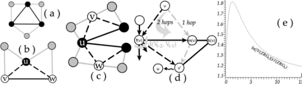
Fig. 1. The graph ZRG0 is a triangle, or cycle of 3 nodes. At each time step, to each edge added at the previous time step, we add a node connected to the endpoints of the edge. This can be seen as adding a triangle to each outer edge. The process is depicted step by step up to ZRG3 (a). A possible instance of BZRGpillustrates the depth and
number of nodes in each of the three probabilistic branches (b). The graph grew for 3 time steps, at the end of which the outcome of the last active branch was not to grow.
3
Deterministic version
In this Section, we consider the version introduced by [6] and defined in the previous Section. We denote by Vt the vertices of ZRGt, and At the vertices
added at step t. We established in [7] that|At| = 3 ∗ 2t−1 for t≥ 1.
Fig. 2. In ZRG1, each of the black initial nodes is connected to two grey added nodes (a). We assume that u∈ At−1, thus it stems from an edge (v, w). As the edges (u, v) and (u, w) are active, u will also be connected to two nodes in At(b). We assume that
u∈ Vt−2: thus, it is connected to two (children) nodes v, w∈ At−1. The edges (u, v) and (u, w) being active, u will also be connected to the two nodes they generate at the next step, belonging to At(c). Shortest paths to compute d(At, Vt−1) (d). The average distance in ZRGtis close to the logarithm of the graph’s size (e).
By construction, a node u ∈ At is connected to the two endpoints of a
formerly active edge. One endpoint was created at the step immediately before (i.e., t−1), and we call it the mother m(u) ∈ At−1, while the other endpoint was
same mother as u is called its uterine brother and denoted as b(u). Furthermore, we observe that each node v ∈ Vt−1 is connected to two nodes of At. This is
proved by induction: it holds for t = 1 (see Figure 2(a)), we assume it holds up to t− 1 and we show in Figure 2(b-c) that it follows for t. Since each node in
Atis connected to two nodes in Vt−1, and each node in Vt−1is connected to two
nodes in At, the graph has a bipartite structure used in our proof.
We now turn to the computation of `(ZRGt). We denote by d(X, Y ) =
P
u∈X
P
v∈Y d(u, v) the sum of distances from all nodes in X to all nodes in Y .
Theorem 1 establishes the value of g(t) = d(Vt, Vt), from which we will establish
the average distance using `(ZRGt) = |V (ZRG g(t)
t)|∗(|V (ZRGt)|−1). We gave the
sketch of a different proof in [7], thus the interested reader can compare it with the full proof given here to better illustrate graph-theoretic techniques.
Theorem 1. g(t) = 4t(6t + 3) + 2∗ 3t
Proof. By definition, Vt= Vt−1∪At. Thus, d(Vt, Vt) = d(Vt−1, Vt−1)+d(At, Vt−1)+
d(Vt−1, At) + d(At, At). Since the underlying graph is undirected, d(At, Vt−1) =
d(Vt−1, At) hence
g(t) = g(t− 1) + 2d(At, Vt−1) + d(At, At), t≥ 2 (1)
In the following, we consider that a shortest path from v∈ At always goes
through f (v), unless the target is the brother b(v) or the mother m(v) in which case correction factors are applied. Suppose that we instead go through m(v) to reach some node u: since m(v) is only connected to b(v), f (v) and some node
v0 (see Figure 2(d)) then the route continues through v0. However, the path
v, m(v), v0 can be replaced by v, f (v), v0 without changing the length.
We compute d(At, Vt−1) for t ≥ 2. Since we always go through f(v), we
use a path of length 2 in order to go from v to m(v) whereas it takes 1 using the direct link. Thus, we have to decrease the distance by 1 for each v∈ At, hence a
correcting factor−|At|. We observe that each node in Vt−2 is the father of two
nodes in At, hence routing through the father costs 2d(Vt−2, Vt−1) to which we
add the number of times we use the edge from v to the father. As each v ∈ At
goes to each w∈ Vt−1, the total cost is
d(At, Vt−1) = 2d(Vt−2, Vt−1) +|At||Vt−1| − |At| (2)
We have that 2d(Vt−2, Vt−1) = 2d(Vt−2, Vt−2) + 2d(Vt−2, At−1) = 2g(t−
2) + 2d(Vt−2, At−1). Furthermore, using Eq. 1 we obtain g(t − 1) = g(t −
2) + 2d(At−1, Vt−2) + d(At−1, At−1)⇔ 2d(At−1, Vt−2) = g(t− 1) − g(t − 2) −
d(At−1, At−1). Substituting these equations with Eq. 2, it follows that
d(At, Vt−1) = g(t− 1) + g(t − 2) − d(At−1, At−1) +|At||Vt−1| − |At| (3)
We compute d(At, At), for t≥ 2. In order to go from v to its uterine brother
b(v)∈ At, it takes 2 hops through their shared mother, whereas it takes 3 hops
through the father. Thus, we have a correction of 1 for |At| nodes. The path
f (w). Finally, we add 2 for the cost of going from a node to its father at both
ends of the path, and we have|At|(|At| − 1) such paths. Thus, the overall cost is
d(At, At) = 4g(t− 2) + 2|At|(|At| − 1) − |At| (4)
We combine. Given that|At| = |Vt−1|, we substitute Eq. 3 into Eq. 1 hence
g(t) = 3g(t− 1) + 2g(t − 2) + d(At, At)− 2d(At−1, At−1) + 2|At|2− 2|At| (5)
From Eq. 4, for t≥ 3 we obtain d(At−1, At−1) = 4g(t−3)+2|At−1|2−3|At−1|.
Given that|At| = 2|At−1|, we substitute d(At−1, At−1) and Eq. 4 in Eq. 5:
g(t) = 3g(t− 1) + 6g(t − 2) − 8g(t − 3) + 3|At|2− 2|At|, t ≥ 3 (6)
We manually count that f (0) = 6, f (1) = 42 and f (2) = 252. Thus the equation can be solved into g(t) = 4t(6t + 3) + 3∗ 2tusing standard software.
Corollary 1. Since |V (ZRGt)| = 3 ∗ 2t [6], it follows from the Theorem that
`(ZRGt) =
4t(6t+3)+3∗2t
3∗2t(3∗2t−1) =
t2t+1+2t+1
3∗2t−1 .
Using this corollary, we obtain limt→∞ln(|V (ZRG`(ZRG t)|)
t) =
3∗ln(2)
2 ≈ 1.03 and
limt→∞
ln(ln(|V (ZRGt)|))
`(ZRGt) ≈ 0. Thus, the average size is almost exactly ln(|V (G)|)
for large t. Since the size of the graph is exponential in t, it is important that the graphs obtained for small values of t have a similar ratio, which is confirmed by the behaviour illustrated in Figure 2(e).
4
Stochastic branch version
As in the previous Section, we are interested in the ratio between the number of nodes and the average path length. In this Section, our approach is in three steps. Firstly, we establish bounds on the depth of branches, defined as the number of times that a branch has grown. Secondly, we study the number of nodes. We find that the number of nodes undergoes a first-order phase transition at the critical probability pc = 0.5: for p < 0.5, there is a finite number of nodes,
whereas for p≥ 0.5 this number becomes infinite. Since in the latter the expected depth of branches is bounded by finite numbers, the expected graphs have an arbitrarily small average distance compared to the number of nodes. However, the expected number of nodes only provides a mean-field behaviour that can may lack representativeness due to a few very large instances. Thus, we conclude by investigating the behavior of instances of bounded depth.
4.1 Depth of branches
To fully characterize the depth of branches, we are interested in their expected depth for the standard case as well as the two extremal cases consisting of the deepest and shallowest branches. In other words, we study the mean-field behaviour and we provide a lower and an upper bound. We start by introducing our notation for the depth in Definition 1. We start by establishing the expected depth of a branch in Theorem 2, then we turn to the expected shallowest depth, and we conclude in Theorem 4 showing that the expected deepest depth of a branch is finite.
Definition 1. We denote D1, D2, D3the depth of the three branches. The depth of the deepest branch is Dmax= max(D1, D2, D3) and the depth of the shallowest branch is Dmin= min(D1, D2, D3).
Theorem 2. The expected depth of a branch isE(Di) = 1−pp , i∈ {1, 2, 3}.
Proof. The probability P (Di = k) that a branch grows to depth k is the
probability pk of successily growing k times, and the probability not to grow once (i.e., to stop at depth k + 1). Thus, P (Di = k) = p| {z }· · · p
k
·(1 − p) = pk(1− p). Since the expected value of a discrete random variable Di is given
by E(Di) =
P∞
k=0(kP (Di = k)), it follows thatE(Di) =
P∞ k=0(kp
k(1− p)) =
p(1− p)P∞k=0(kpk−1). Since dpk
dp = kp
k−1, we further simplify into E(D i) =
p(1− p)P∞k=0(dpdpk). As the sum of a derivative is equal to the derivative of the sum, it follows that E(Di) = p(1− p)
dP∞k=0pk
dp . We note that
P∞
k=0p k is an
infinite geometric sum, hence
E(Di) = p(1− p)dpd 1−p1 = p(1−p)
(1−p)2 =
p
1−p
Theorem 3. E(Dmin) =− p
3
p3−1
Proof. The probability of the shallowest depth to be at least k knowing that the
probability p applies iid to each branch is P (Dmin ≥ k) = P (D1 ≥ k)P (D2 ≥
k)P (D3 ≥ k) = p3k. By definition, P (Dmin = k) = P (Dmin ≥ k) − P (Dmin ≥
k + 1), thus P (D
min = k) = p3k− p3(k+1). This probability is plugged into the
definition of the expected value as in Theorem 2 hence E(Dmin) = P∞ k=0(kP (Dmin = k)) = P∞ k=0(k(p 3k− p3(k+1))) =− p3 p3−1
Theorem 4. E(Dmax) =−
p(p3+4p2+3p+3) (p−1)(p2+p+1)(p+1).
Proof. By construction, the deepest branch does not exceed k iff none of the
branches has a depth exceeding k. Since the probability p applies iid to all three branches, we have P (Dmax ≤ k) = P (D1 ≤ k)P (D2 ≤ k)P (D3 ≤ k).
Furthermore, a branch is strictly deeper than k if it successfully reaches depth k+ 1. Thus, P (Di> k) = p| {z }· · · p k+1 = pk+1, i∈ {1, 2, 3}. By algebraic simplification, we have P (Dmax≤ k) = (1 − P (D1 > k))(1− P (D2 > k))(1− P (D3> k)) = (1− pk+1)3. By definition, P (D max = k) = P (D ≤ k) − P (D ≤ k − 1) =
(1− pk+1)3 − (1 − pk)3. Given that E(D
max) =
P∞
k=0(kP (Dmax = k)), we
replace the expression of P (Dmax = k) to obtain E(Dmax) =
P∞
k=0(k((1−
pk+1)3− (1 − pk)3)). The final expression results from algebraic simplification
4.2 Average number of nodes
We introduce our notation in Definition 2, and Theorem 5 provides a closed-form of the expected number of nodes.
Definition 2. We denote by N1, N2, and N3 the number of nodes in the three branches. Since we start from a cycle with three nodes, the total number of nodes is N = N1+ N2+ N3+ 3.
Theorem 5. For p < 1
2, the expected number of nodes isE(N) = 3(1−p)
1−2p . Proof. First, we focus on the expected number of nodes in a branch. As the
probability p applies iid to all three branches, we select the first branch without loss of generality. By construction, the total number of nodes N1 in the branch
1 at depth D1 = k ≥ 0 is N1 = 2k− 1 =
Pk i=12
i−1. Thus, the expected value
of the random variable N1 is given byE(N1) =
P∞
k=0((2
k− 1)P (D1 = k)). As
shown in Theorem 2, P (D1 = k) = pk(1− p). We replace it in the equation to
obtainE(N1) =
P∞
k=0((2
k−1)pk(1−p)). After expanding the equation, we have
E(N1) = P∞ k=0(2kpk(1−p)−pk(1−p)) = (1−p) P∞ k=0((2p)k)−(1−p) P∞ k=0(pk).
As in Theorem 2, we have P∞k=0(pk) = 1−p1 thus the second term simplifies and yields E(N1) = (1− p)
P∞
k=0((2p)
k)− 1. It is well known that a serie of
the type P∞k=0(xk) diverges to infinity for x ≥ 1. Thus, our serie diverges for
2p≥ 1 ⇔ p ≥ 12. In other words, this results only holds for 0≤ p < 12. The infinite geometric sumP∞k=0((2p)k) can be simplified in 1
1−2p henceE(N1) = 1−p 1−2p− 1 = 1−p−1+2p 1−2p = p
1−2p. The probability p applies iid to all three branches
henceE(N1) =E(N2) =E(N3). Thus, by Definition 2, the expected number of
nodes in the overall graph is given byE(N) = 3 + 3E(N1) = 3 +1−2p3p = 3(1−p)
1−2p .
Theorem 5 proved that the average number of nodes diverges to infinity at the critical probability pc = 0.5. This may appear to be a discrepancy with
Theorem 4 stating that the expected depth of the deepest branch is finitely bounded. For the sake of clarity, we provide an intuition and an example on this point. First, we note that the expected deepest depth and the expected number of nodes have different growth rates. Indeed, even if graphs with very deep depth scarcely occur at p = 0.5, their impact on the expected number of nodes is tremendous since the number of nodes grows exponentially with the depth. On the other hand, the impact of such graphs on the expected deepest depth is only linear. To illustrate different growth rates with a known network, consider the complete graph Kn, in which each of the n≥ 1 nodes is connected to all others. In
Kn, the number of nodes grows linearly whereas the distance is constant. Thus,
the distance between two nodes is 1 even with an infinite number of nodes. In a nutshell, the expected number of nodes for p≥ 0.5 may not be repre-sentative of most instances due to the large impact of very deep graphs. Thus, it remains of interest to investigate the number of nodes for graphs with bounded depths. This is established in Theorem 6, in which we consider the q% possible instances with smallest depth. By lowering the impact of the very deep graphs, this theorem consistutes a lower bound that better describes practical cases.
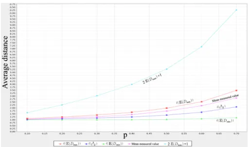
Fig. 3. The measured average distance compared with three bounds and an estimate,
proved or conjectures. The simulations valide the conjectures. Color online.
Fig. 4. Up to p = 0.5 (excluded), the expected number of nodes is finite. From p =
0.5, the expected number of nodes is infinite due to very large instances, thus we provide a finite estimate by considering the q% smallest instances, from q = 75% to
q = 100− 10−3%. Simulations were limited to the graphs that fitted in memory thus the mean measured value represents only an estimate based on small graphs for values beyond p = 0.5. Color online.
Lemma 1. E(N|Dmax≤ K) = −
(3p−6pK+22K+6pK+12K−3)
(2p−1)(pK+1−1
Proof. The expected number of nodes is adapted from Theorem 5 by the
follow-ing substitutions:E (N1) |{z} (N1|Dmax≤K) =P∞k=0((2k−1) P (D 1= k) | {z } P (D1=k|Dmax≤K) ). We simplify: P (D1= k|Dmax≤ K) formula = P (D1=k∩Dmax≤K) P (Dmax≤K) expendDmax = P (D1=k∩D1≤K∩D2≤K∩D3≤K) P (D1≤K∩D2≤K∩D3≤K) independence = P (D1=k)P (D1≤K)P (D2≤K)P (D3≤K) P (D1≤K)P (D2≤K)P (D3≤K) simplifying = P (D1=k) P (D1≤K)
Thus E(N1|Dmax ≤ K) =
P∞
k=0((2
k− 1)P (D1=k)
P (D1≤K)). We showed in the proof
of Theorem 4 that P (D1 ≤ K) = 1 − pK+1, and we showed in the proof of
Theorem 2 that P (D1= k) = pk(1− p). By substituting these results, and using
from the previous Theorem thatE(N) = 3 + 3E(N1), it follows that
E(N|Dmax≤ K) = 3 + 3
PK k=0(
(2k−1)pk(1−p) 1−pK+1 )
The closed form formula follows by algebraic simplification.
Theorem 6. By abuse of notation, we denote by E(N|q) the expected number
of nodes for the q% of instances of BZRGp with smallest depth. We have
E(N|q) = −3(−1+(1−√3q)
ln(2)+ln(p) ln(p) )(p−1)
−√3q(2p−1)
Proof. Theorem 4 proved that the expected deepest depth of a branch was at
most K with probability (1− pK+1)3. Thus, if we want this probability to be q, we have to consider branches whose depth K is at most:
(1− pK+1)3= q⇔ K = log
p(1−√3q)− 1
The Theorem follows by replacing K in Lemma 1 with the value above. The effect of a few percentages of difference in q is shown in Figure 4 together with the results from Theorem 5 and 6. In the inset of Figure 4, we show that the number of nodes grows sharply with q.
4.3 Average path length
We conducted experiments in order to ensure the veracity of the results presented in the two previous Sections, and to compare them with devised bounds. For values of p from 0.1 to 0.7 by steps of 0.1, we measured the average distance of the resulting graphs, obtained as the average over 1000 instances. In Figure 3, we plot it against four bounds and an estimated mean:
Fig. 5. We measured the ratio betweenE(N|100 − 10x) (a), ln(E(N|100 − 10x)) (b), ln(ln(E(N|100 − 10x))) (c) and the diameter 2E(D
max) + 1 for x going from 0 (bottom
curve) to 7 (top curve). We determined a critical probability pc = 0.5 at which the
regime changes, and this is confirmed by these measures showing that the average distance goes from linear in the number of nodes (a) for p < pcto small in the number
of nodes (b) for p≥ pc.
– Proven bound. Theorem 4 established the expected deepest depth. At any time, the graph has three branches, and we can only go from one branch to another through the basic cycle. Thus, the expected maximum distance between any two points in the graph consists of going from the most remote node of two branches to the cycle, and going through the cycle. As a node is at most at distance E(Dmax) from the cycle and we can go from any
node of the cycle to another in one hop, the expected maximum distance is 2E(Dmax) + 1. Since this is the maximum distance, we use it as a proven
upper bound on the average distance.
– Conjecture bounds. Our intuition is that since `(t), proven in Theorem 1, provides the average distance for a graph in which all branches have depth
t, then a lower and upper bound can be obtained by considering the graphs
with shallowest (Theorem 3) and deepest (Theorem 4) depths respectively. This is confirmed by the simulations.
– Conjectured mean. Similarly to the conjecture bounds, we have proven the expected depthE(D) = 1−pp of a branch in Theorem 2, and the simulation confirms that `(1−pp ) constitute an estimate of the average distance. As we previously did for the deterministic version, we now investigate whether the average distance `(BZRGp) can be deemed small compared to the number of
nodes|V |. As explained in the previous Section, we proved a (first-order) phase transition at the critical probability pc = 0.5. The behaviour of the graph can
be characterized using the ratios displayed in Figure 5: for p¿ pc, we observe
an average distance proportional to the number of nodes, and for p > pc− ² the
average distance is proportional to the logarithm of the number of nodes which is deemed small. The ratio in Figure 5(c) is too low, and tends to 0 for a large probability p, thus the graph cannot be considered ultra-small. The separation at pc− ² can also be understood from a theoretical perspective. For p ≥ pc, we
is finite whereas|V | is infinite. When p = 0.5−ε, the average distance is bounded by a finite number: by Theorem 2 we have that the expected depth of a branch is E(Di) < 1 and, using the aforementioned argument regarding the maximum
distance, this entails `(BZRGp) < 2∗ 1 + 1 = 3. Furthermore, as stated in the
proof of Theorem 6, the expected number of nodes in a branch isE(Ni) = 0.5ε−ε
which can thus be arbitrarily large. Thus, the behaviour for p ≥ pc is also
expected to hold in a small neighborhood of the critical probability.
5
Stochastic edge version
In order to show a broad variety of approaches, we prove the number of nodes and the average path length of EZRGp using different tools from the previous
Section. Theorem 7 establishes the number of nodes in the graph.
Theorem 7. For p < 12, the expected number of nodes isE(N) = 3 +1−2p3p . Proof. We consider the dual of the graph, which we define using a visual example
in Figure 6. The dual is a binary tree: for an edge, a triangle is added (root of the tree) with probability p, to which two triangles are added iid at the next step (left and right branches of the tree) with probability p, and so on. Since one node is added to the tree when a node is added to the original graph, studying the number of nodes in EZRGp is equivalent to studying the number of nodes
in the tree. We denote the latter by t(p). The number of nodes starting from any edge is the same, and we denote it by N . Thus, N corresponds to the probability of starting a tree (i.e., adding a first node that will be the root) multipled by the number of nodes in the tree: N = pt(p). Once the tree has been started, the number of nodes corresponds to the sum of the root and the number of nodes in the two branches, hence t(p) = 2pt(p) + 1. Note that there is a solution if and only if p < 12, and otherwise the number of nodes is infinite. By arithmetic simplification, we obtain t(p)(1−2p) = 1 ⇔ t(p) = 1−2p1 . Thus, N = 1−2pp . Since the graph starts as a cycle of length three, the number of counts corresponds to the three original nodes, to which we add the number of nodes starting in each of the three trees, thusE(N) = 3 +1−2p3p = 3(11−2p−p).
A proof similar to Theorem 7 could be applied to the number of nodes in
BZRGp. However, the tree associated with BZRGp grows by a complete level
with probability p, instead of one node at each time. Thus, the current depth of the tree has to be known by the function in order to add the corresponding number of nodes, hence N = pt(p, 0) and t(p, k) = pt(p, k + 1)∗ 2k.
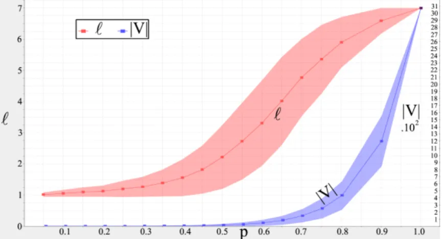
In the previous model, we showed that the expected average distance had a constant growth whereas the expected number of nodes had an exponential growth. Thus, the gap between the two could be arbitrarily large. Using simu-lations reported in Figure 7, we show that the same effect holds in this model.
6
Conclusion and future work
We proved a close-form formula for the average distance in ZRGt. We proposed
Fig. 6. Nodes linked by black edges correspond to four successive growths from an
initial active edge. When a node x is added, it creates a triangle, to which we associate a node ¯x. If two triangles share an edge, their nodes ¯x1and ¯x2are connected by a grey dashed edge. The graph formed by the nodes associated to triangles is called dual.
at the same critical probability. In the recent years, we have witnessed many complex network models in which nodes are added at each time step. The graph-theoretic and probabilistic techniques illustrated in our paper can thus be used to rigorously prove the behaviour of models.
Fig. 7. The average path length has a slow growth compared to the number of nodes,
as in BZRGp. We show the values averaged accross simulations and the standard
deviation. Color online.
References
1. S. Schnettler, Social Networks 31, 165 (July 2009), ISSN 03788733
2. P. Giabbanelli and J. Peters, Technique et Science Informatiques (to appear)(2010) 3. D. J. Watts, Small worlds: the dynamics of networks between order and randomness
(Princeton University Press, Princeton, NJ, 1999)
4. J. Davidsen, H. Ebel, and S. Bornholdt, Phys. Rev. Lett. 88 (2002)
5. Z. Zhang, L. Chen, S. Zhou, L. Fang, J. Guan, and T. Zou, Phys. Rev. E 77 (2008) 6. Z. Zhang, L. Rong, and C. Guo, Physica A 363, 567 (2006)
7. P. Giabbanelli, D. Mazauric, and S. Perennes, in Proc. of the 12th AlgoTel, 2010 8. Z. Zhang, L. Rong, and F. Comellas, J. of Physics A 39, 3253 (2006)