Mathematical study of quantum and classical models for random materials in the atomic scale
312
0
0
Texte intégral
Figure


+7


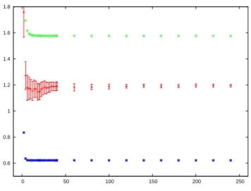


![Figure 1.11: The average of the L 1 (( −∞ , E cut ])-norm of the IDOS N p as a function of p in the rHF model.](https://thumb-eu.123doks.com/thumbv2/123doknet/14670483.741542/57.892.273.604.204.468/figure-average-cut-norm-idos-function-rhf-model.webp)
Documents relatifs
