HAL Id: hal-01418913
https://hal.archives-ouvertes.fr/hal-01418913
Submitted on 17 Dec 2016
HAL is a multi-disciplinary open access
archive for the deposit and dissemination of
sci-entific research documents, whether they are
pub-lished or not. The documents may come from
teaching and research institutions in France or
abroad, or from public or private research centers.
L’archive ouverte pluridisciplinaire HAL, est
destinée au dépôt et à la diffusion de documents
scientifiques de niveau recherche, publiés ou non,
émanant des établissements d’enseignement et de
recherche français ou étrangers, des laboratoires
publics ou privés.
Quantitative Separation Logic and Programs with Lists
Marius Bozga, Radu Iosif, Swann Perarnau
To cite this version:
Marius Bozga, Radu Iosif, Swann Perarnau. Quantitative Separation Logic and Programs with Lists.
The 4th International Joint Conference on Automated Reasoning (IJCAR 2008), Aug 2008, Sydney,
Australia. pp.34-49, �10.1007/978-3-540-71070-7_4�. �hal-01418913�
Quantitative Separation Logic and Programs with Lists
Marius Bozga, Radu Iosif, and Swann Perarnau VERIMAG, 2 Avenue de Vignate, F-38610 Gi`eres
{iosif,bozga,perarnau}@imag.fr
Abstract. This paper presents an extension of a decidable fragment of Separa-tion Logic for singly-linked lists, defined by Berdine, Calcagno and O’Hearn [8]. Our main extension consists in introducing atomic formulae of the form lsk(x,y) describing a list segment of length k, stretching from x to y, where k is a logical variable interpreted over positive natural numbers, that may occur further inside Presburger constraints.
We study the decidability of the full first-order logic combining unrestricted quan-tification of arithmetic and location variables. Although the full logic is found to be undecidable, validity of entailments between formulae with the quantifier pre-fix in the language ∃∗{∃N,∀N}∗is decidable. We provide here a model theoretic
method, based on a parametric notion of shape graphs.
We have implemented our decision technique, providing a fully automated frame-work for the verification of quantitative properties expressed as pre- and post-conditions on programs working on lists and integer counters.
1 Introduction
Separation Logic [15, 21] has recently become a widespread formalism for the specifi-cation of programs with dynamic data structures. Due to the intrinsic complexity of the heap structures allocated and manipulated by such programs, any attempt to formalize their correctness has to be aware of the inherent bounds of undecidability. Indeed, even programs working on simple acyclic lists have the power of Turing machines, and it is expected that a general logic describing sets of configurations reached in such pro-grams has an undecidable satisfiability (or validity) problem. An interesting problem is to define decidable logics that are either specialized for a certain kind of recursive data structures (e.g. lists, trees), or that are restricted by the quantifier prefix.
This paper presents an extension of a decidable fragment of Separation Logic for singly-linked lists, defined by Berdine, Calcagno and O’Hearn [8] and used as an in-ternal representation for sets of states in the Smallfoot tool [4]. Our main extension consists in introducing atomic formulae of the form lsk(x,y) describing a list segment
of length k, stretching from x to y, where k is a logical variable interpreted over positive natural numbers, that may occur further inside Presburger constraints. This is motivated by the need to reason about programs that work on both singly-linked list structures and integer variables (counters). We denote the extended logic as Quantitative Separation Logic (QSL).
In reality, many programs would traverse a list structure, while performing some iterative computation on the integer variables. The result of this computation usually
depends on the number of steps, which, in turn, depends of the length of the list. A specification of the correct behavior for such a program needs to take into account both the lengths of the lists and the values of the counters.
We study the decidability properties of the full first-order logic combining unre-stricted quantification of arithmetic and location variables. Although the full logic is found to be undecidable, validity of entailments between formulae with the quantifier prefix in the language ∃∗{∃N,∀N}∗ is decidable. We provide here a model theoretic
method for decidability, based on a parametric notion of shape graphs. As a byproduct, we obtain a decision procedure for the fragment of Separation Logic considered in [8]. The decision procedure for a fragment ofQSL is currently implemented in the L2CA tool [3], a tool for translating programs with singly-linked lists into bisimilar counter automata, according to the method of [9], which opens the possibility of using well-known counter automata techniques and tools, e.g. [6, 22, 5], in order to verify pre-and post- conditions expressed inQSL, on programs working on both singly-linked lists and integer variables.
1.1 Related Work
The saga of logics for describing heap structures has its roots in the early work of Burstall [11]. Later on, work by Benedikt, Reps and Sagiv [7], Reynolds [21] and Ish-tiaq and O’Hearn [15], has brought the subject into focus, whereas recent advances have been made in tackling the decidability problem [14, 8, 23]. The idea of combin-ing shape and arithmetic specifications arises in the work of Zhang, Sipma and Manna [24], where a combination of free term algebras with Presburger constraints is studied for decidability. The work that is closest to ours is the one of Berdine, Calcagno and O’Hearn [8], which defines a decidable subset of Separation Logic [21] interpreted over singly-linked heap models. The work in this paper is in fact an extension of the logic in [8] with integer variables representing list lengths. One of the main challenges in the present paper was to adapt the model of parametric shape graphs in order to cope with the notion of disjunctive heaps, which is the essence of the semantic model for Separation Logic.
Regarding program analysis, the use of abstract domains (including integers and memory addresses) with quantifiers of the form ∃∗∀∗has been considered in the work
of Gulwani et al. [13, 12]. Unlike our approach, their work is based on using abstrac-tions that prove to be sufficient, in general, for checking correctness of a large body of programs. Some of our examples, such as InsertSort, are also verified using the method of [12]. Recently, Magill et al. [17] report on a program analysis technique that uses Separation Logic [21] extended with first-order arithmetic. However, the main empha-sis of [17] is a program analyempha-sis based on counterexample-driven abstraction refine-ment, whereas our work focuses on distinguishing decidable from undecidable when combining Separation Logic with first-order arithmetic. As a matter of fact, [17] claims that validity of entailments in the purely existential fragment of Separation Logic with the lsk(x,y) predicate and linear constraints is decidable, without giving the proof, by
analogy to the proof-theoretic method from [8]. We extend their result by showing de-cidability of the validity of entailments in the ∃∗{∃N,∀N}∗fragment, versus
undecid-ability of satisfiundecid-ability in the ∃∗∃∗
N(∀ |∀N)∃∗∃∗Nfragment (or equivalently, validity in
the ∀∗∀∗
N(∃ |∃N)∀∗∀∗Nfragment).
Roadmap The paper is organized as follows. Section 2 defines the syntax and semantics of the logic QSL. Section 3 proves the undecidability of the logic, while Section 4 proves the decidability of entailments in the ∃∗{∃N,∀N}∗ fragment. Section 5 gives
some examples of programs verified usingQSL, and Section 6 concludes. For space reasons, all proofs are given in [10].
2 Definitions
In the rest of the paper, for a set A we denote by A⊥the set A ∪ {⊥}. For a function f : A → B, we denote by dom( f ) = {x ∈ A | f (x) (= ⊥} its domain and by img( f ) = {y ∈ B | ∃x ∈ A . f (x) = y} we denote its image. The element ⊥ is used to denote that a (partial) function is undefined at a given point, e.g. f (x) = ⊥. Sometimes we shall use the graph notation for functions, i.e. f = {)a,b*,...} if f (a) = b,..., etc. The notation λx : A.y stands for the function {)x,y* | x ∈ A}, and λx : A.⊥ is the empty function /0, by convention. Let Part(S) denote the set of all partitions of the set S.
By
T
(X) we denote the set of all terms build using variables x ∈ X. For a term (formula)τ(X) and a mapping µ : X →T
(X), we denote byτ[µ] the term (formula) in which each occurrence of x is replaced with µ(x). For a formulaϕ, we denote as FV(ϕ) the set of its free variables. Ifϕ is a formula of the first-order arithmetic of integers, and ν : FV (ϕ) → Z is an interpretation of its free variables, we denote by ν |= ϕ the fact that ϕ[ν] is a valid formula.Presburger arithmetic )N,+,0,1* is the theory of first-order logic of addition and successor function (S(n) = n + 1) [20]. The interpretation of logical variables is the set of natural numbers N, and the meaning of the function symbols 0,1,+ is the natural one. It is well-known that the satisfiability problem for Presburger arithmetic is decidable [20].
u,v,... ∈ PVar program variables x,y,... ∈ LVar location variables k,l,... ∈ IVar integer variables L := nil | u | x location expressions I := n ∈ N | k | I +I integer expressions A := I = I | L = L | emp | L +→ L | lsI(L,L) atomic propositions
F := T | A | ¬F | F ∧ F | F ∗F | ∃x . F | ∃Nk . F formulae
Fig. 1. Separation Logic with Presburger Arithmetic
The syntax ofQSL is given in Figure 1. Notice the difference between program variables PVar and location variables LVar, the former being logical constants, whereas the latter may occur within the scope of a quantifier. Let FVL(ϕ) = FV(ϕ) ∩LVar and
FVI(ϕ) = FV(ϕ) ∩ IVar denote the sets of location and integer free variables of ϕ,
As usual, we defineϕ ∨ ψ= ¬(¬ϕ ∧ ¬ψ), ϕ ⇒ ψ∆ = ¬ϕ ∨ ψ, ∀x . ϕ∆ = ¬∃x . ¬ϕ∆ and ∀Nk . ϕ= ¬∃∆ Nk . ¬ϕ. Moreover, we write k ≤ l and ls(x,y) as shorthands for
∃Nk1.k + k1= l and ∃Nk . lsk(x,y), respectively. F is a shorthand for ¬T. The bounded
quantifiers ∃Nm ≤ n . ϕ(m) and ∀Nm ≤ n . ϕ(m) are used instead of ∃Nm . m ≤ n∧ϕ(m)
and ∀Nm . m ≤ n ⇒ ϕ(m), respectively. We shall also deploy some of the classical
shorthands in Separation Logic: x +→ = ∃y . x +→ y, and x !→ y∆ = x +→ y ∗ T, where∆ y is either a location variable or nil. For list segment formulae we define !lsk(x,y)=∆ lsk(x,y) ∗ T and !ls(x,y)= ls(x,y) ∗ T.∆
The semantics ofQSL formulae is given in terms of heaps. A heap is a rooted graph in which each node has at most one successor. Let Loc denote the set of locations. We assume henceforth that Loc is an infinite, countable set, with a designated element nil ∈ Loc. In what follows, we identify heaps that differ only by a renaming of their locations.
Definition 1. A heap is a pair H = )s,h*, where s : PVar ∪ LVar → Loc⊥ associates
variables with locations, and h : Loc → Loc⊥is the partial successor mapping. In
par-ticular, we have h(nil) = ⊥. We denote by
H
the set of all heaps with variables from PVar ∪ LVar and locations from Loc.The interpretation of a formula is defined by a forcing relation |= between tuples )H,ν,ι* ∈
H
× (LVar +→ Loc⊥) × (IVar +→ N⊥) and formulae. Hereν : LVar → Loc⊥is a partial valuation of location variables, and ι : IVar → N⊥is a partial valuation
of integer variables. The semantics ofQSL formulae is given below, for a given heap H = )s,h*:
[[u]])H,ν*= s(u), [[x]])H,ν*=ν(x), [[nil]])H,ν*= nil
)H,ν,ι* |= T always )H,ν,ι* |= L1= L2 iff [[L1]])H,ν*= [[L2]])H,ν* )H,ν,ι* |= emp iff h = /0 )H,ν,ι* |= L1+→ L2 iff h = {)[[L1]])H,ν*, [[L2]])H,ν**} )H,ν,ι* |= ¬ϕ iff )H,ν,ι* (|= ϕ )H,ν,ι* |= ϕ ∧ ψ iff )H,ν,ι* |= ϕ and )H,ν,ι* |= ψ
)H,ν,ι* |= ϕ ∗ ψ iff there exist H1,H2such that H = H1• H2
and )H1,ν,ι* |= ϕ,)H2,ν,ι* |= ψ
)H,ν,ι* |= ∃x . ϕ iff )H,ν[x ← l],ι* |= ϕ for some l ∈ Loc \ {nil} Here H1• H2denotes the disjoint union of H1= )s,h1* and H2= )s,h2*, i.e, dom(h1) ∩
dom(h2) =/0, h = h1∪ h2. The above definitions are standard in Separation Logic [21].
The rules below are specific to our extension: [[I]]ι= I[ι]
)H,ν,ι* |= I1= I2 iff [[I1]]ι= [[I2]]ι
)H,ν,ι* |= ls0(L1,L2) iff )H,ν,ι* |= L1= L2 ∧ emp
)H,ν,ι* |= lsn+1(L1,L2) iff )H,ν,ι* |= ∃x . lsn(L1,x) ∗ x +→ L2
)H,ν,ι* |= lsI(x,y) iff )H,ν,ι* |= ls[[I]]ι(x,y)
)H,ν,ι* |= ∃Nk .ϕ iff )H,ν,ι[k ← n]* |= ϕ, for some n ∈ N
There are two types of quantifiers, ∃ ranges over locations Loc, and ∃Nover natural
numbers N. A tuple )H,ν,ι* is said to be a model of ϕ iff )H,ν,ι* |= ϕ. If FV(ϕ) = /0, we denote the fact that H is a model ofϕ directly as H |= ϕ. An entailment is a formula of typeϕ ⇒ ψ. Given such an entailment, the validity problem asks if it holds for any tuple )H,ν,ι*, i.e. if any model of ϕ is also a model of ψ.
Note that we use the “classical” (non-intuitionistic) semantics of Separation Logic [15], in which a points-to relation L1+→ L2is true iff the heap is defined on only one
cell whose address is the value of L1. As a result, lsk(L1,L2) is true iff the heap is
defined only on the set of addresses that form the list from L1up to (but not including)
L2. Another consequence of using this semantics is that ls0(L1,L2) is true only on the
empty heap. One can however recover the intuitionistic semantics of [21] by using the shorthands L1!→ L2and !lsk(L1,L2) instead.
The following notion of dangling location is essential for the semantics of Separa-tion Logic on heaps [15, 21]. To understand this point, consider the formulaϕ : (u +→ v) ∗ (v +→ nil), describing a heap H = )s,h*, in which u and v are allocated to two dif-ferent cells, i.e. s(u) = l1, s(v) = l2, and nothing else is in the domain of the heap, i.e.
h = {)l1,l2*,)l2,nil*}. The reason for which H |= ϕ, is that there exists two disjoint
heaps, namely H1= )s,{)l1,l2*}* and H2= )s,{)l2,nil*}*, such that H1|= u +→ v and
H2|= v +→ nil. Notice the role of the location l2, pointed to by the variable v, which is
referenced by the first heap, but allocated in the second one. This location ensures that the disjoint union of H1and H2is defined, and that H1• H2|= u +→ v ∗ v +→ nil.
Definition 2. A location l ∈ Loc \ {nil} is said to be dangling in a heap H = )s,h* iff l ∈ (img(s) ∪ img(h)) \ dom(h).
In the following, we denote by dng(H) the set of all dangling nodes of H, and by loc(H) = img(s) ∪ dom(h) ∪ img(h) the set of all locations, either defined or dangling in H.
2.1 Motivating Example
Let us consider the program in Figure 2. The loop on the left hand side inserts elements into the list pointed to by u, while incrementing the c counter, and the loop on the right removes the elements in reversed order, while decrementing c. The pre- and post-condition of the program are inserted as Hoare-style annotations. Both initially and finally, the value of c is zero and the heap is empty.
In order to prove that the program terminates without a null pointer dereferencing, and moreover ensuring that the post-condition holds, one needs to relate the value of c to the length of the list pointed to by u, as it is done in the invariants of the left and right
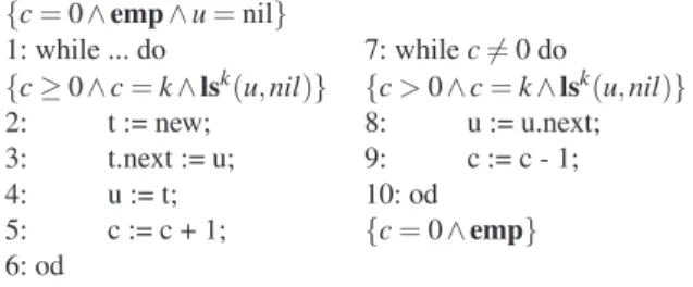
{c = 0 ∧ emp ∧ u = nil} 1: while ... do {c ≥ 0 ∧ c = k ∧ lsk(u,nil)} 2: t := new; 3: t.next := u; 4: u := t; 5: c := c + 1; 6: od 7: while c (= 0 do {c > 0 ∧ c = k ∧ lsk(u,nil)} 8: u := u.next; 9: c := c - 1; 10: od {c = 0 ∧ emp}
Fig. 2. Program verification using QSL
hand side : c = k ∧ lsk(u,nil). This example could not be handled using standard
Sep-aration Logic, since we explicitly need the ability of reasoning about both list lengths and integer variables.
3 Undecidability of QSL
In this section we prove the undecidability of theQSL logic. Namely the class of for-mulae with quantifier prefix in the language ∃∗∃∗
N(∀ | ∀N)∃∗∃∗Nare shown to have an
undecidable satisfiability problem. It is to be noticed that undecidability ofQSL is not a direct consequence of the undecidability of Separation Logic [19], since the proof in [19] uses multiple selector heaps, while in this case we consider only heaps composed of singly-linked lists. Our result is non-trivial since it is well-known also that, even sim-ple logics, e.g. FOL, MSOL are decidable when interpreted over singly-linked lists, and become quickly undecidable when interpreted over grid-like, and more general graph structures.
Theorem 1. The set of QSL formulae which, written in prenex normal form, have the quantifier prefix in the language ∃∗∃∗
N(∀ |∀N)∃∗∃∗N, is undecidable.
The idea of the proof is that one can encode all terminating runs of an arbitrary 2-counter machine [18] by a formula ofQSL in the ∃∗∃∗
N(∀ | ∀N)∃∗∃∗Nquantifier
frag-ment. Since the halting problem is undecidable for 2-counter machines, the satisfiability of formulae in the above mentioned fragment is also undecidable.
In the following developments, we shall prove that logical entailment in the ∃∗{∃N,∀N}∗
fragment ofQSL is decidable. We have found no argument for (un)decidability con-cerning the quantifier prefix fragment {∃,∀}∗{∃N,∀N}∗. In particular, all attempts to
reduce (from) to known fragments of MSO with cardinality constraints [16] have failed.
4 Model Theoretic Method
The validity of an entailmentϕ ⇒ ψ is equivalent to the non-satisfiability of the formula ϕ ∧ ¬ψ, i.e. there should be no tuples )H,ν,ι* such that )H,ν,ι* |= ϕ and )H,ν,ι* (|= ψ. Our main result, leading immediately to decidability of entailments, is that, if ϕ is
of the form ∃x1. . .∃xnQ1l1. . .Qmlm .θ(x,l), with Qi ∈ {∃N,∀N} and θ is a boolean
combination of predicates with ¬, ∧ and ∗, all models )H,ν,ι* of ϕ can be represented using a finite number of (finite) structures called symbolic graph representations (SGR). The decision procedure for the validity of a QSL entailmentϕ ⇒ ψ is based on the following idea. We first define operators on sets of SGRs that are the counterparts of the logical connectives ∨, ∧, ∗ and the existential quantifiers ∃x, ∃Nx. Second, for each
existential QSL formulaϕ, we compute a set [[ϕ]] of SGRs that represent all models of ϕ. The construction of this set is recursive, on the structure of ϕ. The entailment ϕ ⇒ ψ is valid iff the set [[ϕ]] 5 [[ψ]] is empty, where 5 is an operator defined on SGRs, that computes the representation of the difference between the set of concrete models of theϕ and the one of ψ. Least, the emptiness problem for sets of SGRs is shown to be decidable, by reduction to the satisfiability problem for the Presburger arithmetic.
4.1 Symbolic Shape Graphs
In this section we define a finite representation of (possibly infinite) sets of heaps, called symbolic shape graphs (SSG), which is the essence of our decision method. The next section defines the SGR representation for sets of heaps, which is based on SSGs and arithmetic constraints.
Definition 3. Given a heap H = )s,h* ∈
H
, a location l ∈ Loc is said to be a cut point in H if either l ∈ img(s)∪dng(H)∪{nil}, or there exists two distinct locations l1,l2∈ Locsuch that h(l1) = h(l2) = l.
A location l is a cut point in a heap if either (1) l is pointed to directly by a program variable, i.e. l ∈ img(s), (2) l is dangling or nil, or (3) l has more than one predecessor in the heap. We denote by l1!Hl2the fact that h(l1) = l2and l2(= ⊥ is not a cut point
in H. Let ∼Hdenote the reflexive, symmetric and transitive closure of the !H relation,
i.e. the smallest equivalence relation that includes !H, and [l]∼be the equivalence class
of l ∈ Loc w.r.t. ∼H. We also refer to these equivalence classes as to list segments. By
convention, we have [⊥]∼= ⊥. Let H/∼= )s/∼,h/∼* be the quotient heap, where:
– s/∼: PVar ∪ LVar → Loc/∼⊥and s/∼(u) = [s(u)]∼, for all u ∈ PVar,
– h/∼: Loc/∼→ Loc/∼⊥and for all l ∈ dom(h), if h(l) = l1and l1is either ⊥ or a cut
point in )s,h*, then h/∼([l]) = [l1]∼. In particular, h/∼([l]) = ⊥, for all l (∈ dom(h).
Note that s/∼and h/∼are well-defined functions. We extend the rest of notations to
quo-tient heaps, i.e. dng(H/∼) = {[l]∼| l ∈ dng(H)} and loc(H/ ∼) = {[l]∼| l ∈ loc(H)}.
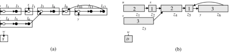
For example, in the heap from Figure 3 (a), the cut points are marked by hollow nodes and the ∼-equivalence classes are enclosed in solid boxes. The quotient heap is the heap in which these boxes are taken as nodes, instead of the individual locations. Definition 4. Given a set PVar of program variables, a set LVar of location variables, and a set of counters
Z
= {z1, . . . ,zn}, a symbolic shape graph (SSG) is a tuple G =)N,D,R,Z,S,V *, where:
– N is a finite set of symbolic nodes, with a designated node Nil ∈ N, – D ⊆ N is a set of symbolic dangling nodes,
– R ⊆ N is a set of symbolic root nodes,
– Z : N \ D →
Z
is an injective function assigning each non-dangling node to a counter,– S : N → N⊥is the successor function, where:
• S(Nil) = ⊥ and S(d) = ⊥, for all d ∈ D, • S(n) (∈ R, for all n ∈ N,
• S(n) ∈ N, for all n ∈ N \ (D ∪ {Nil}).
– V : PVar ∪ LVar → N assigns program and location variables with nodes.
Intuitively, each node of a SSG represents a list segment of a concrete heap. The node Nil stands for the concrete nil location, and each symbolic dangling node repre-sents one dangling location.
Definition 5. An SSG G = )N,D,R,Z,S,V* is said to be in normal form if:
– each node in n ∈ N \{Nil} is reachable either from V(u), for some u ∈ PVar∪LVar, or from some symbolic root r ∈ R, and
– either n ∈ img(V)∪D∪{Nil}, or there exist two distinct nodes n1,n2∈ N such that
S(n1) = S(n2) = n.
S
kdenotes the set of SSGs in normal form, with |R| ≤ k and img(V) ⊆ PVar ∪ LVar.Sometimes we denote by
S
the unionSk∈NS
k. We identify SSGs which are equivalentunder renaming of nodes and counters. The following was proved in [9]:
Lemma 1. Let G = )N,D,R,Z,S,V* ∈
S
kbe a normal form SSG. Then, |N| ≤ 2(|dom(V)|+|R|). As a consequence, the number of such SSGs is bounded asymptotically by 2(|PVar| + |LVar| + k)2(|PVar|+|LVar|+k), and the bound is tight.
The following definition relates the notions of heap and SSG.
Definition 6. Let G = )N,D,R,Z,S,V* ∈
S
be a SSG,ν : dom(V) ∩ LVar → dom(h) a valuation of the location variables of G, and ι : img(Z) → N+ a valuation of thecounters in G. Let H = )s,h* ∈
H
be a heap such that dom(s) = dom(V) ∩ PVar, and H/∼= )s/∼,h/∼* be the quotient of H with respect to ∼H. We say that H is the)ν,ι*-concretization of G iff there exists a bijective mappingη : N⊥→ (loc(h/∼) ∪ {nil,⊥})
such that:
– η(Nil) = {nil} and η(⊥) = ⊥, – η(V (u)) = s/∼(u), for all u ∈ PVar,
– η(S(n)) = h/∼(η(n)), for all n ∈ N \ D,
– η(n) ∈ dng(H/∼), for all n ∈ D,
– ι(Z(n)) = |η(n)|, for all n ∈ N \ D.
We recall upon the fact that heaps are identical, up to isomorphism, which implies that a )ν,ι* is uniquely defined. We say that H is a concretization of G if there exist ν, ι such that H is the )ν,ι*-concretization of G. Roughly speaking, the )ν,ι*-concretization of a SSG G is the heap obtained by replacing each node n of G with a list segment whose length equals the value of the counter Z(n). Moreover, if G has a )ν,ι*-concretization,
2 1 2 1 3 3 (a) (b) y v u w X x z1 z2 z5 z6 z3 w z4 u v x y D l1 l2 l3 l7 l8 l9 l10 l11 l12 l4 l5 l6
Fig. 3. SSG and Concretization
we must haveι(Z(n)) > 0, for all non-dangling symbolic nodes n ∈ N. Notice also that dangling locations are represented by symbolic dangling nodes. We denote byγν,ι(G)
the )ν,ι*-concretization of G and by Γ(G) the set of all concretizations of G.
For example, the SSG in Figure 3 (b) has as )ν,ι*-concretization the heap in Figure 3 (a), for the valuations:
– ν(x) = l3,ν(y) = l10, and
– ι(z1) = 2,ι(z2) = 1,ι(z3) = 3,ι(z4) = 2,ι(z5) = 1,ι(z6) = 3.
Notice that the symbolic dangling node pointed to by w corresponds to a dangling lo-cation pointed to by w in Figure 3 (a).
The following result expresses the fact that one heap may not be the concretization of two different (non-isomorphic) SSGs:
Lemma 2. For two non-isomorphic SSGs G1,G2∈
S
, we haveΓ(G1) ∩ Γ(G2) =/0.4.2 Symbolic Graph Representations
In this section we introduce the notion of symbolic graph representation (SGR) together with a number of operators on these structures. In the next section, we shall provide a stepwise translation of aQSL formula with quantifier prefix ∃∗{∃N,∀N}∗into a set of
symbolic graph representations.
A symbolic graph representation is a pair )G,ϕ*, where G = )N,D,R,Z,S,V * is a SSG in normal form andϕ an open formula over the counters of G, i.e. FV(ϕ) ⊆ img(Z). By
G
we denote the set of all SGRs R = )G,ϕ*, where G ∈S
and the set of counters in each G is a subset ofZ
.A heap H = )s,h* is the )ν,ι*-concretization of )G,ϕ* iff ν : dom(V) ∩ LVar → dom(h) is a valuation of the location variables of G, andι : img(Z) → N+is a valuation
of the counters in G that satisfiesϕ, i.e. ι |= ϕ. This is denoted in the following as H = γν,ι()G,ϕ*). Γ()G,ϕ*) denotes the set of all )ν,ι*-concretizations of )G,ϕ*. The
nota-tion is lifted to finite sets of SGRs in the obvious way:Γ({R1, . . . ,Rn}) =Sni=1Γ(Ri).
We introduce now three operators on finite sets of SGRs, that correspond to the boolean operators of union, intersection and set difference. Let S1,S2⊆
G
be two finiteS18 S2 = {)G,ϕ1∨ ϕ2* | )G,ϕ1* ∈ S1and )G,ϕ2* ∈ S2} ∪
{)G,ϕ* ∈ S1| )G, * (∈ S2} ∪ {)G,ϕ* ∈ S2| )G, * (∈ S1}
S19 S2 = {)G,ϕ1∧ ϕ2* |) G,ϕ1* ∈ S1and )G,ϕ2* ∈ S2}
S15 S2= {)G,ϕ1∧ ¬ϕ2* |) G,ϕ1* ∈ S1and )G,ϕ2* ∈ S2}
∪ {)G,ϕ* ∈ S1| )G, * (∈ S2}
Here the notation )G, * stands for any SGR pair having G as its first component. Let G = )N,D,R,Z,S,V * and notice that, since FV (ϕ1) ⊆ img(Z) and FV(ϕ2) ⊆ img(Z),
then FV (ϕ1∨ ϕ2), FV (ϕ1∧ ϕ2) and FV(ϕ1∧ ¬ϕ2) are also subsets of img(Z).
Lemma 3. SGRs are effectively closed under union, intersection and difference. In par-ticular, we haveΓ(S18 S2) =Γ(S1) ∪ Γ(S2),Γ(S19 S2) =Γ(S1) ∩ Γ(S2) andΓ(S15
S2) =Γ(S1) \ Γ(S2).
The ! operator is defined on SGRs with the following meaning : for two SGRs R1
and R2, we haveΓ(R1! R2) = {H1• H2| H1∈ Γ(R1) and H2∈ Γ(R2)}. In other words,
! is the SGR counterpart of the disjoint union operator on heaps. However, ! is not a total operator, i.e. it is not defined for any pair of SGRs, but only for the ones complying with the following definition :
Definition 7. Two SSGs Gi= )Ni,Di,Zi,Si,Vi*, i = 1,2 are said to match iff there exists
a mapping µ : D1∪D2→ (N1∪N2)⊥such that, for all u ∈ dom(V1)∩dom(V2), either:
– V1(u) ∈ D1and µ(V1(u)) = V2(u), or
– V2(u) ∈ D2and µ(V2(u)) = V1(u).
and µ(d) = ⊥, for all d ∈ (D1∪ D2) \ (dom(V1) ∩ dom(V2)).
Intuitively, two SSGs match if it is possible to relate any dangling node pointed to by program variable in one SSG to a node pointed to by the same variable in the other SSG. Note that two SSGs do not match if the same variable points to some non-dangling node in both. Figure 4 gives an example of two matching SSGs (a) and (b) together with the mapping µ between their nodes (in dotted lines). According to Definition (7), the choice of µ is not unique.
Given two SGRs R1= )G1,ϕ1* and R2= )G2,ϕ2*, with matching underlying SSGs
Gi= )Ni,Di,Zi,Si,Vi*, (for the purposes of this definition, we can assume w.l.o.g. that
N1∩ N2= {Nil} and img(Z1) ∩ img(Z2) =/0), we define R1! R2= )G,ϕ1∧ ϕ2*, G =
)N,D,Z,S,V *, where: – N = (N1∪ N2) \ dom(µ), – D = (D1∪ D2) \ dom(µ), – R = (R1∪ R2) \ dom(µ), – Z = Z1∪ Z2, – for all n ∈ N: S(n) ="µ(SSi(n) if n ∈ Niand Si(n) (∈ dom(µ) i(n)) if n ∈ Niand Si(n) ∈ dom(µ) i = 1,2
(b) (a) (c) u D D v w v D D u w u D v w µ µ µ Fig. 4. Matching SSGs – for all u ∈ dom(V1) ∪ dom(V2):
V (u) = " V
i(u) if Vi(u) (∈ dom(µ)
µ(Vi(u)) if Vi(u) ∈ dom(µ) i = 1,2
For example, the SSG in Figure 4 (c) is the result of the !-composition of the SSGs in Figure 4 (a) and (b).
The ! operator is undefined, if G1and G2 do not match. Notice that if G1∈
S
k1,G2∈
S
k2 and )G,ϕ* = )G1,ϕ1* ! )G2,ϕ2*, then G ∈S
k1+k2. The correctness of thedefinition is captured by the following Lemma:
Lemma 4. Given two SGRs R1= )G1,ϕ1* and R2= )G2,ϕ2*, such that G1 and G2
match, we haveΓ(R1! R2) = {H1• H2| H1∈ Γ(R1), H2∈ Γ(R2)}.
The following projection operator captures the effect of dropping one location vari-able out of the heap. Let R = )G,ϕ* be an SGR, where G = )N,D,R,Z,S,V* is the underlying SSG, and x ∈ img(V) ∩ LVar be a location variable occurring in G. For an arbitrary symbolic node n ∈ N, let precG(n) = {m ∈ N | m (= n, S(m) = n} be the set of
predecessors of n, different from itself, in G.
We define R↓xto be the SGR, having a normal-form underlying SSG (cf. Definition
4), from which x is missing. Formally, let R↓x= )G1,ϕ1*, where:
1. if x (∈ dom(V) then G1= G andϕ1=ϕ.
2. else, if x ∈ dom(V) and either:
(a) there exists u ∈ dom(V) \ {x} such that V(u) = V(x), or
(b) there exist m1,m2∈ dom(S) s.t. m1(= m2and S(m1) = S(m2) = V(x)
then G1= )N,D,R,Z,S,V[x ← ⊥]* and ϕ1=ϕ.
3. else, if x ∈ dom(V), V(x) = n, and for all u ∈ dom(V)\{x}, we have V (u) (= n, and either:
(a) precG(n) = /0, then G1= )N,D,R ∪ {n},Z,S,V[x ← ⊥]* and ϕ1=ϕ, or
(b) n ∈ D and precG(n) (= /0, then G1= )N,D,R,Z,S,V[x ← ⊥]* and ϕ1=ϕ,
(c) n (∈ D and m ∈ precG(n), where Z(m) = k1and Z(n) = k2, then
G1= )N \ {n},D,R,Z[m ← k3][n ← ⊥],S[m ← S(n)][n ← ⊥],V[x ← ⊥]* and
The correctness of this definition is captured in the following Lemma:
Lemma 5. Let R = )G,ϕ* be a SGR, G = )N,D,Z,S,V* be its underlying SSG, and x ∈ LVar be a location variable. Then Γ(R↓x) = {)s[x ← ⊥],h* | )s,h* ∈ Γ(R)}.
Given a set S of SGRs, the emptiness problemΓ(S) = /0 is effectively decidable if all constraintsϕ occurring within elements )G,ϕ* ∈
G
are written in a logic decid-able for satisfiability. In our case, this logic is the Presburger arithmetic, for which the satisfiability problem is known to be decidable [20].4.3 From Formulae to Sets of SGR
We are now ready to describe the construction of a set of SGRs for a given formula : ϕ : ∃x1. . .∃xnQ1l1. . .Qmlm.θ(x,l)
where Qi∈ {∃N,∀N} and θ is a quantifier-free QSL formula. The construction is
per-formed incrementally, following the structure of the abstract syntax tree ofθ. The set x = {x1, . . . ,xn} is called from now on the support set of θ. Without losing generality, we
consider that the leaves of this tree are atomic propositions of one of the forms : T, emp, x = y, x +→ y and lsl(x,y), where x ∈ x∪PVar, y ∈ x∪PVar ∪{nil} and l ∈ {l1, . . . ,lm}.
From now on, let
S
k(x) be the set of all SSGs with at most k root nodes, supportvariables from PVar ∪ x, and counters from a fixed given set
Z
. Given a formulaϕ, we denote by [[ϕ]]x(k) the set of SGRs with at most k root nodes, over the support set x, defining the models ofϕ, in the following sense. The set of concrete heaps correspond-ing to [[ϕ]]x(k) is exactly the set of models ofϕ.For atomic spatial propositions, [[ϕ]]x(k) is computed according to the definitions from Table 1. In the definition of [[emp]]x(k) we consider as parameter the partition )Y1, . . . ,Yp* ∈ Part(x). That is [[emp]]x(k) =S)Y1,...,Yp*∈Part(x)[[emp]]Y1,...,Yp, where [[emp]]Y1,...,Yp
is defined in Table 1. Intuitively, Yi, 1 ≤ i ≤ p is the set of variables that are aliased,
pointing to the same dangling node di, in the empty heap. In Table 1, let D = {d1, . . . ,dp−1},
R = /0 and ∆ =Sp−1
i=1 λx : Yi.di∪ λx : Yp.Nil.
Since emp denotes all heaps with empty domain, in the SGR representation there are no symbolic nodes, which are not dangling or nil. Moreover, there are no counters, and therefore, no arithmetic constraints.
In the definition of [[ϕ]]x(k) for x +→ nil and x +→ y, we consider two parameters: (1) a set Z ⊆ x ∪ {x}, such that x ∈ Z, and (2) a partition )Y1, . . . ,Yp* ∈ Part(x \ Z).
In other words, we have [[ϕ]]x(k) =S{[[ϕ]]YZ1,...,Yp | Z ⊆ x ∪ {x}, x ∈ Z, )Y1, . . . ,Yp* ∈
Part(x\Z)}, where [[ϕ]]Y1,...,Yp
Z is defined in Table 1. Intuitively, Z corresponds to the set
of support variables that are aliased with x in some concrete model, and )Y1, . . . ,Yp* is
used with the same meaning as in the previous definition of [[emp]]x(k).
We recall upon the fact that the models of the atomic propositions x +→ nil and x +→ y are all heaps whose domains consists of only one address, which is the value of x. Therefore the SGR representation uses one non-dangling node n to which one counter z1is mapped. The associated constraint sets z1= 1, according to the semantics.
In the definition of [[lsl(x,nil)]]
x(k) we consider an ordered sequence of disjoint
Zj=/0, for all 1 ≤ i < j ≤ k. Similarly, in the definition of [[lsl(x,y)]]x(k) we consider
sets Z1, . . . ,Zk, where Zi⊆ x ∪ {x,y}, 1 ≤ k ≤ n, such that x ∈ Z1, y ∈ Zk, and Zi∩
Zj=/0, for all 1 ≤ i < j ≤ k. In both cases, we consider also a partition )Y1, . . . ,Yp* ∈
Part(x \ (Sk
i=1Zi)). Intuitively, Z1, . . . ,Zk correspond to the sets of support variables
that are aliased while pointing to the same node in the list, in some concrete model, and )Y1, . . . ,Yp* is used with the same meaning as in the previous definition of [[emp]]x(k).
Since the models of lsk(x,nil) and lsl(x,y) are all heaps defined only on the
ad-dresses of the nodes in the list pointed to by x, we represent them by a list of symbolic non-dangling nodes n1, . . . ,nk, where all variables from Zipoint to ni, 1 ≤ i ≤ k. Each
node nihas an associated counter zi, and the sum of the values of zimust equal l.
More-over, if x points to the end (nil or y) of the list, the length l must be zero.
[[emp]]Y1,...,Yp [[x +→ nil]]Y1,...,Yp
Z [[x +→ y]]YZ1,...,Yp [[lsl(x,nil)]]YZ11,...,Y,...,Zpk [[ls
l(x,y)]]Y1,...,Yp
Z1,...,Zk
N D ∪ {Nil} D ∪ {n,Nil} D ∪ {n,Nil} D ∪ {n1, . . . ,nk,Nil} D ∪ {n1, . . . ,nk,Nil}
Z /0 {)n,z1*} {)n,z1*} {)ni,zi*}ki=1 {)ni,zi*}ki=1
S /0 {)n,Nil*} {)n,dk*}, if y ∈ Yk{)ni,ni+1*}i=1k−1∪ {)nk,Nil*} {)ni,ni+1*}k−1i=1
V ∆ λx : Z.n∪∆ λx : Z.n∪∆ Sk
i=1λx : Zi.ni∪ ∆ Ski=1λx : Zi.ni∪ ∆
ϕ < z1= 1 z1= 1 ∑i=1k zk= l ∧ ∑ki=1zk= l ∧
(x ∈ Zk→ l = 0) (x,y ∈ Zk→ l = 0)
Table 1. SGR for atomic spatial propositions
The pure formulae x = nil (x = y) correspond to sets of SGRs are the ones in which x points to nil (y), and the counters occur unconstrained. Their SGR semantics is defined as follows:
[[x = nil]]x(k) = {)G,<* | G = )N,D,R,Z,S,V* ∈
S
k(x), V(x) = Nil}[[x = y]]x(k) = {)G,<* | G = )N,D,R,Z,S,V* ∈
S
k(x), V(x) = V(y)}The SGR semantics for the QSL connectives is defined as follows: [[T]]x(k) = {)G,<* | G ∈
S
k(x)}[[ψ1∧ ψ2]]x(k) = [[ψ1]]x(k) 9 [[ψ2]]x(k)
[[¬ψ]]x(k) = {)G,<* | G ∈
S
k(x)} 5 [[ψ]]x(k)[[ψ1∗ ψ2]]x(k) = [[ψ1]]x(k) ! [[ψ2]]x(k)
Ifπ is a purely arithmetic formula, then we have:
[[ψ ∧π]]x(k) = {)G,θ ∧ π* | )G,θ* ∈ [[ψ]]x(k)}
The semantics for the existential quantifiers is as follows:
[[∃x . ψ]]x(k) = {R↓x | R ∈ [[ψ]]x∪{x}(k − 1)}, k ≥ 1
[[∃Nl .ψ]]x(k) = {)G,∃l . θ* |) G,θ* ∈ [[ψ]]x(k)}
Lemma 6. Given ϕ a QSL formula containing only numeric quantifiers (∃N, ∀N),
and {x1, . . . ,xn} ⊆ FVL(ϕ), we have, for all valuations ν : FVL(ϕ) \ {x1, . . . ,xn} →
Loc, andι : FVI(ϕ) → N+:Γν,ι#[[∃x1. . .∃xn.ϕ]]FVL(ϕ)\{x1,...,xn}(n)
$
= {H | )H,ν,ι* |= ∃x1. . .∃xn.ϕ}
Theorem 2. The validity of entailments between formulae in the ∃∗{∃N,∀N}∗
quanti-fier fragment ofQSL is a decidable problem.
The proof of Theorem 2 uses the fact that the set of models for each formula in the ∃∗{∃N,∀N}∗quantifier fragment ofQSL can be finitely represented using a set of SGRs
(cf. Lemma 6). An entailmentϕ ⇒ ψ is valid if and only if the set of models of the for-mulaϕ ∧¬ψ is empty. The latter is given by the set of SGRs encoding the set-theoretic difference between the models ofϕ and the models of ψ. Since the emptiness of this set is decidable, by reduction to Presburger arithmetic, the validity of the entailment is also decidable.
According to Lemma 1, the number of SSGs that can be generated using N variables is of the order of
O
(NN). However, the number of SSGs encountered in practice isrelatively small, since in principle, the explosion occurs only due to the unrestricted use of negation and the T proposition, which can be easily avoided.
5 Application of the Model Theoretic Method for QSL
The translation betweenQSL formulae with quantifier prefix of the form ∃∗{∃N,∀N}∗
and sets of SGRs gives a method for deciding the validity of entailments in this logic. Moreover, there is another, more practical advantage to this approach, that gives us a effective method for the verification of both shape and numeric properties of programs with lists.
The L2CA tool [3] is a tool for verifying safety and termination properties of pro-grams with singly-linked lists, based on the translation of propro-grams into counter au-tomata [9]. A counter automaton generated by L2CA has control states of the form )l,G*, where l is a control label of the original program, and G is a SSG over the set PVar of pointer variables of the input program. By Lemma 1, the set of control states of a counter automaton generated by L2CA is finite, which guarantees that each program with lists will be translated into a finite-control counter automaton. The semantics (set of runs) of the counter automaton generated by L2CA is in a bisimulation relation with the semantics of the original program, therefore all results of the analysis of the counter automaton (e.g. safety properties, termination) carry over to the original program.
The fact that any ∃∗{∃N,∀N}∗QSL formula ϕ corresponds to a set [[ϕ]] of pairs
)G,ψ*, where G is an SSG and ψ is a Presburger constraint, allows us to extend the L2CA tool to check total correctness of Hoare triples in which the pre- and post-conditions are expressed as ∃∗{∃N,∀N}∗QSL formulae. Suppose that {ϕ} P {ψ} is
such a triple. Then for each SGR )Gk,φk* ∈ [[ϕ]] the L2CA tool will generate a counter
automaton Akwith initial state )l0,Gk*, where l0is the initial control label of the
pro-gramP. This automaton corresponds to the semantics of P when started in an initial control state )l0,H0*, where H0∈ Γ()Gk,φk*). Let A be the union of all such Ak.
By using a combination of existing tools for the analysis of counter automata, e.g. [6, 2, 1] we can verify whether A, started in each control state )l0,Gk* with values of
counters satisfying the Presburger constraintφk, reaches a final control state )lf,Gf*
with the counters satisfying some Presburger constraintφ1 such that |= φ → φ1, for
some )Gf,φ1* ∈ [[ψ]]. This suffices for checking partial correctness. On what concerns
total correctness, we use a termination analysis tool for counter automata, e.g. [1], to check whetherP, started with any heap H0such that H0|= ϕ, terminates.
5.1 Experimental Results
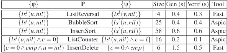
Table 2 presents some experimental results of verifying Hoare triples of the form {ϕ} P {ψ}, whereϕ and ψ are QSL formulae, and P is a program handling lists. The ListReversal example receives in input a non-circular list pointed to by u of length l and returns a non-circular list pointed to by v containing the cells of the first list in reversed order. The BubbleSort and InsertSort programs are classical sorting algorithms for which we verified that the length of the input list stays the same. The ListCounter example is a simple loop traversing a list pointed to by u, while incrementing an integer counter c. InsertDelete is the example from Figure 2.
{ϕ} P {ψ} Size Gen (s) Verif (s) Tool {lsl(u,nil)} ListReversal {lsl(v,nil)} 4 0.4 0.3 Fast {lsl(u,nil)} BubbleSort {lsl(u,nil)} 25 0.4 0.4 Aspic {lsl(u,nil)} InsertSort {lsl(u,nil)} 58 0.6 0.6 Aspic {lsl(u,nil) ∧c = 0} ListCounter {lsl(u,nil) ∧c = l} 16 0.2 0.1 Aspic
{c = 0 ∧ emp ∧ u = nil} InsertDelete {c = 0 ∧ emp} 6 1.5 0.5 Fast Table 2. Experimental Results using the L2CA and ASPIC tools
For all examples, the size (number of control locations) of the automata generated by L2CA is given in the second (Size) column, the time needed for generation in the third (Gen) column, and the time needed to verify partial correctness of the model is given in the fourth (Verif) column. The tool used (either Aspic [2] or Fast [6]) is given in the fifth column. All programs were found to be correct.
6 Conclusions
We have developed an extension of Separation Logic interpreted over singly-linked heaps, that allows to specify properties related to the sizes of the lists. This logic is especially useful for reasoning about programs that combine dynamically allocated data with variables ranging over integer domains.
The decidability of the extended logic is studied, the full quantifier fragment being shown to be undecidable, by a reduction from the halting problem for 2 counter ma-chines. However the validity of entailments in the ∃∗{∃N,∀N}∗fragment of the logic
1In general this is an over-approximation of the set of reachable configurations, obtained using
is decidable, which allows the use this fragment to specify Hoare triples for programs with lists. The verification of total correctness properties specified in this way was made possible by an extension of the L2CA tool.
References
1. ARMC. http://www.mpi-sb.mpg.de/˜rybal/armc/.
2. ASPIC. http://www-verimag.imag.fr/˜gonnord/aspic/aspic.html. 3. L2CA. http://www-verimag.imag.fr/˜async/L2CA/l2ca.html.
4. Smallfoot. http://www.dcs.qmul.ac.uk/research/logic/theory/projects/smallfoot/index.html. 5. A. Annichini, A. Bouajjani, and M.Sighireanu. Trex: A tool for reachability analysis of
complex systems. In Proc.CAV, volume 2102 of LNCS, pages 368 – 372. Springer, 2001. 6. S. Bardin, A. Finkel, J. Leroux, and L. Petrucci. Fast: Fast accelereation of symbolic
transi-tion systems. In Proc. TACAS, volume 2725 of LNCS. Springer, 2004.
7. M. Benedikt, T. Reps, and M. Sagiv. A decidable logic for describing linked data structures. In Springer Verlag, editor, Proc. European Symposium On Programming. LNCS, 1999. 8. J. Berdine, C. Calcagno, and P. O’Hearn. A Decidable Fragment of Separation Logic. In
FSTTCS, volume 3328 of LNCS, 2004.
9. A. Bouajjani, M. Bozga, P. Habermehl, R. Iosif, P. Moro, and T. Vojnar. Programs with lists are counter automata. In Springer Verlag, editor, Proc. Computer Aided Verification (CAV). LNCS, 2006.
10. M. Bozga, R. Iosif, and S. Perarnau. Quantitative separation logic and programs with lists. Technical Report TR 2007-9, VERIMAG, 2007.
11. R. M. Burstall. Some techniques for proving correctness of programs which alter data struc-tures. Machine Intelligence, 7:23–50, 1972.
12. S. Gulwani, B. McCloskey, and A. Tiwari. Lifting abstract interpreters to quantified logical domains. In Proc. 35th ACM SIGPLAN-SIGACT symposium on Principles of programming languages. ACM, 2008.
13. S. Gulwani and A. Tiwari. An abstract domain for analyzing heap-manipulating low-level software. In Proc. Intl. Conference on Computer Aided Verification, 2007.
14. N. Immerman, A. Rabinovich, T. Reps, M. Sagiv, and G. Yorsh. Verification via Structure Simulation. In CAV, volume 3114 of LNCS, 2004.
15. S. Ishtiaq and P. O’Hearn. BI as an assertion language for mutable data structures. In POPL, 2001.
16. F. Klaedtke and H. Ruess. Monadic second-order logics with cardinalities. In Proc.30th International Colloquium on Automata, Languages and Programming. LNCS, 2003. 17. S. Magill, J. Berdine, E. Clarke, and B. Cook. Arithmetic Strengthening for Shape Analysis.
In SAS, volume 4634 of LNCS, 2007.
18. M. Minsky. Computation: Finite and Infinite Machines. Prentice-Hall, 1967.
19. P. O’Hearn, C. Calcagno, and H. Yang. Computability and Complexity Results for a Spatial Assertion Language for Data Structures. In FSTTCS, volume 2245 of LNCS, 2001. 20. M. Presburger. ¨Uber die Vollstandigkeit eines gewissen Systems der Arithmetik. Comptes
rendus du I Congr´es des Pays Slaves, Warsaw 1929.
21. J. C. Reynolds. Separation logic: A logic for shared mutable data structures. In Springer Verlag, editor, Proc. 17th IEEE Symposium on Logic in Computer Science. LNCS, 2002. 22. P. Wolper and B. Boigelot. Verifying systems with infinite but regular state spaces. In Proc.
CAV, volume 1427 of LNCS, pages 88–97. Springer, 1998.
23. G. Yorsh, A. Rabinovich, M. Sagiv, A. Meyer, and A. Bouajjani. A logic of reachable pat-terns in linked data-structures. In Proc. Foundations of Software Science and Computation Structures. LNCS, 2006.
24. T. Zhang, H. Sipma, and Z. Manna. Decision procedures for recursive data structures with integer constraints. In Proc. Intl. Joint Conference of Automated Reasoning, 2004.