Publisher’s version / Version de l'éditeur:
Vous avez des questions? Nous pouvons vous aider. Pour communiquer directement avec un auteur, consultez la première page de la revue dans laquelle son article a été publié afin de trouver ses coordonnées. Si vous n’arrivez pas à les repérer, communiquez avec nous à [email protected].
Questions? Contact the NRC Publications Archive team at
[email protected]. If you wish to email the authors directly, please see the first page of the publication for their contact information.
https://publications-cnrc.canada.ca/fra/droits
L’accès à ce site Web et l’utilisation de son contenu sont assujettis aux conditions présentées dans le site LISEZ CES CONDITIONS ATTENTIVEMENT AVANT D’UTILISER CE SITE WEB.
Oceans '08 [Proceedings], 2008
READ THESE TERMS AND CONDITIONS CAREFULLY BEFORE USING THIS WEBSITE. https://nrc-publications.canada.ca/eng/copyright
NRC Publications Archive Record / Notice des Archives des publications du CNRC :
https://nrc-publications.canada.ca/eng/view/object/?id=bffedcb0-43b5-4195-83f6-07170f54993e
https://publications-cnrc.canada.ca/fra/voir/objet/?id=bffedcb0-43b5-4195-83f6-07170f54993e
NRC Publications Archive
Archives des publications du CNRC
This publication could be one of several versions: author’s original, accepted manuscript or the publisher’s version. / La version de cette publication peut être l’une des suivantes : la version prépublication de l’auteur, la version acceptée du manuscrit ou la version de l’éditeur.
Access and use of this website and the material on it are subject to the Terms and Conditions set forth at
Progress in predicting the performance of ocean gliders from at-sea
measurements
Progress in Predicting the Performance of Ocean
Gliders from At-Sea Measurements
Christopher D. Williams
∗, Ralf Bachmayer
†, Brad deYoung
‡∗ National Research Council Canada
Institute for Ocean Technology St. John’s, NL, A1B 3T5, Canada email: [email protected]
† Memorial University of Newfoundland
Faculty of Engineering and Applied Science St. John’s, NL, A1B 3X5, Canada
email: [email protected]
‡ Memorial University of Newfoundland
Department of Physics and Physical Oceanography St. John’s, NL, A1B 3X7, Canada
email: [email protected]
Abstract— With over 100 commercially-available ocean gliders
being used by researchers around the world, there is strong evidence that these platforms have become the tool of choice for those who require continuous sampling of ocean properties over a range of user-controllable depths. Researchers continue to add new sensors to these vehicles usually on the external surfaces where a sensor can work in an essentially unobstructed flow condition. These added sensors change the behaviour of the glider. For the purpose of improving our predictions of the behaviour of a glider during steady-state glides and course-changing manoeuvres, it is useful to have a simple analytical hydrodynamic model which can be validated quickly using at-sea measurements during several descending and ascending glides.
The purpose of this paper is twofold: (i) to show how the hydrodynamic properties which govern steady-state gliding can be extracted from measurements made with on-board sensors, and, (ii) to show how these hydrodynamic properties can be used to predict the performance of ocean gliders (e.g. glide angle, glide speed, duration of voyage etc.). We describe a three-parameter model which has proved useful in representing the behaviour of an ocean glider during straight-line descents and ascents. This parametric model has been validated with at-sea measurements during multiple glides. Estimates for these parameters can be obtained from the measurements of four quantities on-board a Slocum ElectricTM glider, namely (i) the fore-and-aft position of the pitch-control battery, (ii) the volume of seawater which is ingested or expelled by the buoyancy engine, (iii) the glider pitch angle, and, (iv) the glider depth. We describe briefly a method for obtaining estimates for three of these parameters and show some results in terms of the glider drag and lift coefficients over a wide range of operating conditions. Additional work is outlined to obtain estimates for the parameters which determine the pitching moment behaviour of this ocean glider.
I. INTRODUCTION
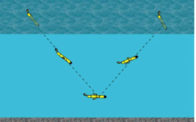
Increasingly ocean gliders are becoming the tool of choice for researchers who require continuous sampling of ocean properties. These gliders operate by changing their net weight in seawater thus gliding downward when they are heavier that the surrounding fluid and upward when they are lighter than
it. The resulting trajectory is a saw-tooth pattern as shown diagrammatically in Fig 1. The first designs appeared in [1] and have evolved into the Slocum ElectricTM gliders which
have been commercially available from the Webb Research Corporation for some years [2]. Recently the SeagliderTM[3]
and SprayTM[4] have become commercially available. Various
models of gliders have depth limits of 200, 500, 1000 m if based on aluminum pressure hulls while composite-material hulls have been designed to operate at depths up to 6000 m [5] and [6].
All three of these gliders use batteries to energize the on-board sensors as well as the buoyancy-change and trajectory-control devices e.g. electric pump to change buoyancy, fore-and-aft sliding battery pack to change pitch angle, rolling battery pack to change bank angle, rudder actuator etc. With an overall mass of about 50 kg, the "Slocum Electric" 200 m glider has a proven duration of up to 40 days when equipped with the basic sensors payload while versions with additional sensors will have a corresponding shorter duration.
In contrast the Slocum ThermalTMglider extracts the
major-ity of its energy from the vertical variations in the temperature of seawater. With a depth rating of 2000 m, this thermal glider has a projected operational duration of up to five years and a range of 40,000 km [7] and [8].
Section II describes the motivation for this investigation and provides some background information. Section III provides experimental results that are applicable to gliders. Section IV describes some recent at-sea experiments. Section V describes the analytical model and shows some results. Section VI de-scribes some recent experiments and provides some data from recent glider voyages. Section VII presents some conclusions, Section VIII some applications, and, Sections IX and X outline our future research.
II. MOTIVATION ANDBACKGROUND
The basis of this investigation can be divided into two processes, what we will refer to as the forward process and the inverse process. The forward process is concerned with the prediction of the behaviour of an ocean glider using known values of four hydrodynamic parameters (a,b,c,d) which con-trol gliding; see §III, equations (1) to (3). The inverse process is concerned with finding values for the controlling parameters (a,b,c,d) from sensor measurements during in-water experi-ments with several "Slocum Electric" gliders.
The impetus to develop this prediction method arose due to the need to add new sensors to existing gliders. Since most flow-through sensors (such as the conductivity, temper-ature and depth (CTD) and dissolved oxygen units) must be mounted on the exterior of the hull, it is natural to expect that the hydrodynamic properties of the glider will change from that of the base-line glider configuration. Thus a combination of an experimental method, an analytical model and a data-analysis technique must be developed in order to quickly categorize the changes to vehicle hydrodynamics which are due to the additional externally-mounted sensors. For example, in a typical configuration the CTD sensor is mounted on the port side of the hull below the wing; this implies that there will be an additional component to the total drag force which will be due to the presence of the exposed CTD sensor and which will cause the glider to tend to turn to port, with the resulting consequence that a corresponding deflection of the rudder will be required to maintain a straight-ahead glide. A series of steady-state glides in calm water will then show that the higher drag force due to the CTD sensor will result in (i) a slower glide speed, (ii) a different glide angle, (iii) a slower rate of vertical descent, (iv) a slower horizontal speed-over-ground, and, (v) a non-zero rudder angle for straight-ahead gliding. In addition, the resulting analytical model can be used to show that, aside from the additional electrical energy that will be consumed by the CTD sensor, some additional electrical energy will be consumed by the rudder actuator which will result in a shorter-duration voyage. These results suggest that in order to evaluate the hydrodynamic effect of a particular externally-mounted sensor, we require (i) a simple calm-water gliding experiment, (ii) a simple analytical model for the hydrodynamic forces and moment which act on the glider during steady-state glides, and, (iii) a simple data-analysis technique which will extract the necessary hydrodynamic parameters from the measurements made by the on-board sensors during these glides. The primary purpose of this paper is to show how these three items can be accomplished.
Figure 1 shows one simplified dive and climb cycle. When the glider is negatively buoyant it descends along a relatively straight glide path at an approximately constant pitch angle, subject of course to local ocean current conditions. Similarly, when the glider is positively buoyant it ascends along a relatively straight glide path. The change from descent to ascent occurs when the glider’s altimeter indicates that the glider is typically 20 m above the seabed. When the glider
Fig. 1. Example saw-tooth pattern for gliding
Fig. 2. Launching a glider over the side of a small fishing vessel
comes to the ocean surface, the air bladder in the tail section is automatically inflated and the tail projects above the sea surface thus improving the quality of the line-of-sight radio-frequency or satellite communications.
Figure 2 shows a single person launching a glider over the side of a small fishing vessel. Due to its limited size and weight, such a glider can easily be launched and recovered over the side of inflatable boat.
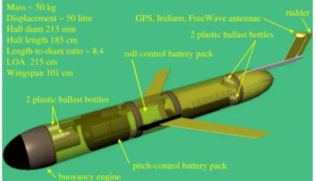
Figure 3 shows a CAD rendering of the ballasting and control mechanisms inside a Slocum electric glider. This glider has a mass of about 50 kg, displaces about 50 litre of seawater; the hull diameter is 213 mm, and, the hull length is 185 cm which provides a hull length-to-diameter ratio of about 8.4. The overall length is 215 cm while the wingspan is 101 cm. This glider contains two small port-and-starboard plastic ballast bottles at the forward upper end, and, two small top-and-bottom plastic ballast bottles at the aft end of the hull. An 8 kg battery pack slides fore-and-aft under servo control in order to achieve the desired vehicle pitch angle. In the Slocum Electric gliders, only a manual adjustment of the roll-control battery pack is possible so this adjustment is included in the ballasting procedure [9] thus there is no roll control actuator or sensor for battery roll position. The "dome" on top of the fixed portion of the vertical fin contains the antennae for the GPS, Iridium and FreeWave communications systems. The aft
2 plastic ballast bottles
2 plastic ballast bottles
pitch-control battery pack
rudder GPS, Iridium, FreeWave antennae
roll-control battery pack
buoyancy engine Mass ~ 50 kg Displacement ~ 50 litre Hull diam 213 mm Hull length 185 cm Length-to-diam ratio ~ 8.4 LOA 215 cm Wingspan 101 cm
Fig. 3. Ballasting and control mechanisms inside a Slocum Electric glider
Time between surfacings
Fig. 4. Typical glider measurements of depth and altitude above the seabed
portion of the vertical fin is a moveable rudder, which is used under servo control to achieve a desired heading.
Figure 4 shows some results from Conception Bay from July 2006 in terms of the measured glider depth versus time since deployment; the data are shown for a period of about five hours. Here the glider was programmed to descend to a maximum depth of 180 m and to return to the surface for a GPS position update after about one hour. On the first dive the seabed was detected at a depth of about 160 m so the glider turned around at a depth of about 150 m. Subsequent dives indicate that the seafloor rises to a depth of about 85 m along the chosen transect. The red arrows along the top edge of the figure indicate the time between surfacings, which is user-selected and is typically two to three hours.
Figure 5 shows a map of the north-eastern portion of the island of Newfoundland. For voyage 215, glider #049 was launched from a small vessel in Trinity Bay. The glider was programmed to travel via a sequence of way-points along a relatively straight transect to the north-east out over the Newfoundland Shelf and to return in a similar fashion into Conception Bay for recovery. The blue line shows our longest deployment to date, a voyage which lasted 21 days and transited 500 km horizontally. The direction and extent of this voyage were designed to replicate a portion of the
Fig. 5. Voyage 215, 26 July to 16 August 2006
Department of Fisheries and Oceans (DFO) Bonavista Line (red line) which is sampled on a regular basis using tradi-tional ship-borne instruments, thus permitting a comparison of measurements made using the two sampling methods. While the glider provides essentially continuously-sampled data, the ship-based measurements are taken at stations 15 km apart. Thus the glider provides a larger data set with lower capital and deployment costs.
III. HYDRODYNAMICLOADS ONGLIDERHULLS
Figure 6 shows the bare hull of a small full-scale AUV being tested in the NRC-IOT towing tank using the Planar Motion Mechanism (PMM). This apparatus is used to measure the hydrodynamic loads which are exerted on the hull during (i) towing at fixed yaw angles, (ii) oscillatory sway and yaw manoeuvres, and, (iii) portions of constant-radius turns. In November 2005 we performed a series of experiments in the NRC-IOT towing tank with the bare hull of a small, full-scale AUV. The purpose of these experiments was to categorize the contribution of the hull alone to the total hydrodynamic loads which the glider experiences during steady-state gliding; the contributions of wing, tail-boom, rudder and antenna can be added using traditional aerodynamic techniques. The PMM apparatus permits forced oscillations at prescribed frequencies and amplitude during towing. The resulting trajectories in space are typically sinusoidal in shape, for both sway or yaw manoeuvres. In these experiments five models of identical maximum diameter and different lengths were used, see Figure 7.
The five models used a common constant-diameter mid-body of diameter 203 mm to which nose and tail sections were attached. Pairs of equal-length spacers were used to set the length of each model. Table 1 summarizes the geometric properties of the five models; LDR is the length-to-diameter ratio.
Fig. 6. A Phoenix AUV model (bare hull) suspended from the NRC-IOT Planar Motion Mechanism in the towing tank
A3 A2 A1 F3 F2 F1 L/D = 12.5 A3 A2 F3 F2 L/D = 11.5 A1 A3 F3 F1 L/D = 10.5 A3 F3 L/D = 9.5 L/D = 8.5 Nose Mid-body Tail
Fig. 7. The five bare-hull model configurations
LDR LOA [mm] MC (nose) [mm] LCB (nose) [mm] Ratio MC to LOA Ratio LCB to LOA 8.5 1724 736 815 0.427 0.473 9.5 1927 838 915 0.435 0.475 10.5 2130 940 1017 0.441 0.477 11.5 2333 1041 1118 0.446 0.479 12.5 2536 1143 1220 0.451 0.481 TABLE I
PARTICULARS OF THE FIVE MODELS TESTED: LDRIS THE LENGTH-TO-DIAMETER RATIO, LOAIS THE OVERALL LENGTH, MCIS THE MOMENT CENTRE AT THE ORIGIN, LCBIS THE DISTANCE TO THE CENTRE OF BUOYANCY(CB). ALL HULL DIAMETERS ARE203MM.
The common mid-body contained a strut-mounted three-component balance which measured the axial force (AF), lat-eral force (SF) and yaw moment (YM) about a fixed transverse
-200 -10 0 10 20 0.2 0.4 0.6 0.8 1
Angle of attack [deg]
D ra g c o e ff ic ie n t C D f o r la rg e a n g le s
Phoenix models final coefficients based on frontal area
LDR 8.5 LDR 9.5 LDR 10.5 LDR 11.5 LDR 12.5
Fig. 8. Drag coefficient CD for the five models
-20 -10 0 10 20 -2 -1 0 1 2
Angle of attack [deg]
L if t c o e ff ic ie n t C L f o r la rg e a n g le s
Phoenix models final coefficients based on frontal area
LDR 8.5 LDR 9.5 LDR 10.5 LDR 11.5 LDR 12.5
Fig. 9. Lift coefficient CL for the five models
axis; the measured moments were later transferred to an axis through the centre of buoyancy (CB) for each model. The results from a series of static (fixed) yaw angle experiments over a range of ±20◦are shown below. The next three figures
show the results of converting these balance measurements to the drag force, lift force and pitching moment coefficients required for our analytical glider model.
The lift and drag forces were non-dimensionalized using the frontal area of the mid-body, πd2
/4, while the pitching moment was non-dimensionalized using the product of the frontal area and the overall hull length.
Figure 8 shows the drag coefficient, CD, versus angle of attack, AOA, for the full measurement range, for the five hull lengths. As expected, the longer models have the larger drag coefficients, due to the skin friction acting on the larger surface area.
Figure 9 shows the lift coefficient, CL, vs AOA, for the full measurement range, for the five hull lengths. As expected, the longer models have the larger lift coefficients.
Figure 10 shows the pitch moment coefficient, CM (about an axis through the CB), vs AOA, for the five hull lengths, for the full measurement range. As expected, the longer models
-20 -10 0 10 20 -0.4 -0.3 -0.2 -0.1 0 0.1 0.2 0.3 0.4
Angle of attack [deg]
P it c h m o m e n t c o e ff ic ie n t a b o u t C B f o r la rg e a n g le
sPhoenix models final coefficients based on frontal area LDR 8.5
LDR 9.5 LDR 10.5 LDR 11.5 LDR 12.5
Fig. 10. Moment coefficient CM about an axis through the CB for each of the five models
have the larger moment coefficients.
The full range of measurements for these bare hulls in terms of the AOA was for ±20◦but they show the form of the curves
which would be obtained for a complete glider, that is, an axi-symmetric hull to which wings and tail have been added.
In the hydrodynamic modelling which follows, there are four parameters (a,b,c,d) which define the hydrodynamic be-haviour of a complete glider, for small AOA. Our analytical modelling uses the following expressions for the hydrody-namic loads in the vertical plane.
CL(AOA) = a · AOA (1)
CD(AOA) = b + c · AOA2
(2)
CM (AOA; CB) = d · AOA (3)
These are approximate expressions for the hydrodynamic loads which were measured for the five bare hulls; these expressions represent only the loads within the limited range of ±10◦since
it will be shown later from the at-sea glider experiments that typically the AOA is small during straight-line glides.
IV. RESULTS FROMAT-SEAEXPERIMENTS
During steady-state gliding four quantities are measured and recorded on-board the glider. Two of these quantities are independently-controlled variables and two are dependent variables. The two independently-controlled variables are (i) the measured instantaneous fore-and-aft position of the pitch-control battery, and, (ii) the volume of seawater ballast which is ingested or expelled by the buoyancy engine. This volume of seawater ballast is inferred from the measured position of the actuator which controls the position of the piston within the buoyancy engine. This piston position is therefore a measure of the net weight (W-B) of the glider; here ‘W’ is the dry weight of the glider (in air) and ‘B’ is the buoyant force which
acts on the glider when it is completely submerged. The two dependent variables are (iii) the measured instantaneous glider pitch angle ‘θ’, and, (iv) the instantaneous depth as determined from measurements of the hydrostatic pressure using a pres-sure transducer. This depth signal can be differentiated in order to obtain the vertical rate of descent and ascent,Vz.
Voyage 193, from July 2006, provides measured values from 52 descents and ascents to a maximum depth of 190 m. This voyage represents a total of 38 hours in the water. The values used in this analysis are average values computed for each descent and ascent; each ascent and descent was assumed to be in a straight line and to be free of any effects of ocean currents. Typical descents take about 8.9 minutes and typical ascents take about 7.2 minutes.
We use an iterative scheme to obtain estimates for the four hydrodynamic parameters (a,b,c,d) identified above which categorize the gliding behaviour for small angles of attack, −10◦ < AOA <+10◦.
V. ITERATIVESCHEME
The following is an example of how the present iterative scheme is employed to obtain the three values (a,b,c).
Step 1. Obtain initial estimates for the values (a,b,c); these may be obtained from a previous descent or ascent with the same glider in the same test configuration. Call these initial estimates(a0, b0, c0).
Step 2. Estimate a starting value for the angle of attack, ‘AOA0’, by using a cubic approximation for the relation
AOA = f0(θm, a0, b0, c0) (4)
Call this value ‘AOA0’. Hereθmis the measured glider pitch
angle.
Step 3. Estimate a new value for the parameter ‘a’ using the exact expression for the relation
a1= f1(Vz, W −B, ρ, Af, b0, c0, AOA0) (5)
Call this value ‘a1’. Here ‘Af’ is the frontal area of the glider
hull,πd2
/4.
Step 4. Estimate a new value for the parameter ‘b’ from the exact expression for the relation
b1= f2(θm, AOA0, a1, c0) (6)
Call this value ‘b1’.
Step 5. Estimate a new value for the parameter ‘c’ from the exact expression for the relation
c1= f3(θm, AOA0, a1, b1) (7)
Call this value ‘c1’.
Step 6. Obtain a new value for the AOA, that is, ‘AOA1’
by using the cubic approximationf0(θm, a1, b1, c1).
Step 7. Obtain a new value for the the parame-ter ‘a’, that is, ‘a2’ by using the exact expression
f1(Vz, W −B, ρ, Af, b1, c1, AOA1).
Step 8. Obtain a new value for the the parameter ‘b’, that is, ‘b2’ by using the exact expressionf2(θm, AOA1, a2, c1).
−30 −20 −10 0 10 20 30 29 30 31 32 33 34 35
Measured mean pitch angle [deg]
Iterated glide path angle [deg]
Steep dive Medium dive Shallow dive Shallow climb Medium climb Steep climb
Fig. 11. Glide path angle vs glider pitch angle
Step 9. Obtain a new value for the the parameter ‘c’, that is, ‘c2’ by using the exact expressionf3(θm, AOA1, a2, b2).
Continue this sequence of ‘n’ steps until the values of (a,b,c) converge to a suitably stable triplet (an, bn, cn).
VI. RESULTS FROM THEITERATIVEMETHOD
Figure 11 shows one set of results of the iterative method, as applied to the data from voyage 193. Here the calculated glide path angle is plotted versus the mean of the measured glider pitch angle, for each of the 50 descents and 51 ascents. The data are shown for six categories of glide angle: steep, medium and shallow descents, and, shallow, medium and steep ascents. The 50 dives show glide path angles in the range from 29◦ to 35◦ which correspond to glider mean pitch angles of
from about −30◦to −20◦, respectively. Since the AOA is the
difference between the glide path angle and the glider pitch angle, the AOA during descent ranges from about 5◦ to 9◦.
Similarly, the 51 ascents show calculated glide path angles in the range from 29◦ to 35◦ which correspond to glider mean
pitch angles of from about+20◦ to+30◦, respectively, again
with the AOA between5◦ and9◦.
Figure 12 shows the corresponding values of the calculated glider speed along the glide path plotted versus the mean measured glider pitch angle. Again the six categories of glides are shown. Here the glide speeds during descent vary from about 39 to 52 cm/s while those during ascents vary from about 42 to 56 cm/s. Clearly the glider was ballasted "light" relative to the surrounding seawater thus the seawater was more dense than the target density used during the pre-voyage ballasting process [9]; this is also corroborated by typical descent and ascent times of 8.9 and 7.2 minutes, respectively.
Figure 13 shows the corresponding values of the drag coefficient, CD, based on the frontal area, plotted versus the deduced AOA, for the six categories of glides used in the two previous figures. The data points for the 50 descents form the basis for the upper curve while those for the 51 ascents form the lower curve. Curves of the form given in equation (2) were fitted in order to extract values for the parameters ‘b’ and ‘c’. For glider 049 in the configuration tested, the minimum drag
−30 −20 −10 0 10 20 30 0.38 0.4 0.42 0.44 0.46 0.48 0.5 0.52 0.54 0.56
Measured mean pitch angle [deg]
Iterated velocity along glide path Vo [m/s]
Steep dive Medium dive Shallow dive Shallow climb Medium climb Steep climb
Fig. 12. Glide speed vs glider pitch angle
0 2 4 6 8 10 0.2 0.25 0.3 0.35 0.4 0.45
Iterated angle of attack [deg]
Iterated drag coefficient CD based on frontal area
Number dive samples 50 Parameter b 0.246 Parameter c 6.18
Number climb samples 51 Parameter b 0.189 Parameter c 6.54 Steep dive Medium dive Shallow dive Fit dives Shallow climb Medium climb Steep climb Fit climbs
Fig. 13. Fitted relations for drag coefficient
coefficient ‘b’ during descents is expected to be about 0.25 while that for ascents is about 0.19. The curvature parameter ‘c’ is about 6.2 for descents and 6.5 during ascents.
Figure 14 shows the corresponding values of the lift co-efficient, CL, based on the frontal area, plotted versus the deduced AOA, for the six categories of glides used in the previous figures. Again the data points for the 50 descents form the basis for the upper curve while those for the 51 ascents form the lower curve. Straight lines of the form given by equation (1) were fitted. For glider 049 in the configuration tested, the lift curve slope ‘a’ was about 4.7 per degree during descents and was about 4.0 per degree during ascents. The sample correlation coefficient for both cases was about 0.98.
Figures 13 and 14 show that the calculated angles of attack range from about5◦ to 10◦ during these 101 separate glides
of duration from 7 to 9 minutes.
VII. CONCLUSIONS
Our focus at NRC-IOT is on the engineering development of underwater vehicles. In this role we add new sensors to ocean gliders. Once a new sensor has been integrated into an existing glider, the question becomes: How to categorize the new hydrodynamic behaviour? For this purpose we have
0 2 4 6 8 10 0 0.1 0.2 0.3 0.4 0.5 0.6 0.7 0.8
Iterated angle of attack [deg]
Iterated lift coefficient CL based on frontal area
Number of samples 50 Slope 4.67 SCC 0.984 Number of samples 51 Slope 3.96 SCC 0.983 Steep dive Medium dive Shallow dive Fit dives Shallow climb Medium climb Steep climb Fit climbs
Fig. 14. Fitted relations for lift coefficient
developed a new iterative procedure for estimating the four lift, drag and pitching moment parameters (a,b,c,d); the procedure for estimating (a,b,c) is detailed in §V.
The resulting glider drag and lift coefficients shown in Figures 13 and 14 indicate that a consistent set of values can be found which represent well the hydrodynamic behaviour of a particular glider over a range of operating conditions. It is evident that the values of these parameters during descents is different from the values which categorize the glider’s behaviour during ascents; this is a typical observation and is due to the ballasting procedure outlined in [9].
VIII. APPLICATIONS
The results from this investigation can be used to improve our predictions of the behaviour of ocean gliders during steady-state glides. This information can be used to provide better predictions of the amount of battery energy which will be consumed during a particular mission, once the number of pumping (buoyancy-changing) events is determined. The more accurately we know the values of these hydrodynamic parameters, the greater confidence we have in our predictions of the likely duration of a mission. This leads to better mission planning and to the development of improved ded-reckoning algorithms. In addition, we can extract higher-quality data from the sensor measurements during the post-processing phase where the measured glider motions can be used to compensate for the dynamical response of the sensors [10].
IX. FUTUREEXPERIMENTALWORK
In the near future we intend to proceed with the following experimental work.
a. Add an acoustic beacon to the underside of a glider. Use the acoustic tracking system in the towing tank or pond to measure the glide path angle directly from the trajectory rather than having to infer the glide path angle from the iterative calculation scheme noted above.
b. Add an acoustic Doppler current profiler (ADCP) to the underside of a glider. Turn the ADCP ‘on’ when the glider is at the ocean surface (and, potentially at a set of
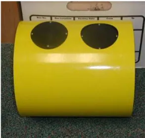
Fig. 15. Glider payload module for four puck-size sensors
Downward-looking acoustic Doppler current profiler (ADCP) Acoustic pinger Upward-looking sonar
Fig. 16. A glider equipped with an ADCP
pre-determined depths) in order to measure the current profile below the glider. Figure 15 shows the new payload module for a "Slocum Electric" glider which can accommodate four puck-sized sensors. Figure 16 shows a new 400 kHz ADCP mounted in one of these gliders; this ADCP can measure the current to depths of the order of 75 m below the glider.
c. Install a MicroStrainTM motion-sensing unit (three rate
gyros, three translational accelerometers) inside a glider. When the glider is at the ocean surface, it will then be able to measure the drift due to wind and waves using the difference of several GPS-determined positions, and, to infer the wave heights and wavelengths using the measured motions of the glider.
d. Add a small multi-beam sonar and downward-looking camera to the underside of a glider. These devices will be used to take "snapshots" during the transition from dive to climb at instants when the vehicle is level and parallel to the seabed. This may be an energy-intensive exercise due to lighting requirements but it may provide a series of seabed images that would be difficult and expensive to obtain otherwise.
X. FUTUREANALYTICAL ANDNUMERICALWORK
Progress in developing a numerical simulator for the Slocum ElectricTMglider using at-sea data for validation was reported
in [11]. As a result of the need for additional validation data and techniques we intend to proceed with the following analytical and numerical work.
a. Use the equilibrium of the hydrostatic pitching moment (due to changes in battery position and amount of ballast pumped) with the hydrodynamic pitching moment (due to hull, wings, tail) in an algorithm which will estimate the fourth parameter ‘d’ for the moment coefficient in equation (3). It appears that this method will also provide estimates of how far the centre of gravity (CG) is vertically below the centre of buoyancy (CB) when the glider is correctly trimmed in pitch and roll [9].
b. Extend the analysis to motions of the submerged glider in the lateral plane e.g. sway, yaw and roll motions. Develop a method to use the on-board measured translational and angular accelerations (away from the otherwise steady straight-line glide path conditions) to infer the magnitude and direction of the ocean current, on an instant-by-instant basis.
ACKNOWLEDGEMENTS
The authors thank the staff and students at NRC-IOT and Memorial University who have assisted in the preparation of the gliders for the various voyages, and, the various funding agencies which have contributed to the success of this research program. Without their continuing support these measure-ments, analysis, conclusions and recommendations would not have been possible.
REFERENCES
[1] Douglas C. Webb. Thermal engine and glider entries. Notebook No. 2, pages 254 & 255, 02 August 1986. Cited in [2].
[2] Clayton Jones and Doug Webb. Slocum Gliders, Advancing Oceanogra-phy. In Proceedings of the 15th International Symposium on Unmanned Untethered Submersible Technology conference (UUST’07), Durham, NH, USA, 19 to 20 August 2007. AUSI.
[3] C.C.Eriksen, T.J.Osse, R.D.Light, T.Wen and T.W.Lehman. Seaglider: A long-range autonomous underwater vehicle for oceanographic research. IEEE Journal of Oceanic Engineering, 26:424–436, October 2001. [4] J.Sherman, R.E.Davis, W.B.Owens and J.Valdes. The autonomous
underwater glider Spray. IEEE Journal of Oceanic Engineering, 26:437– 446, October 2001.
[5] T. James Osse and Charles C. Eriksen. The Deepglider: A full ocean depth glider for oceanographic research. In Proceedings of the OCEANS 2007 conference, Vancouver BC, Canada, 01 to 04 October 2007. MTS/IEEE.
[6] T. James Osse and Timothy J. Lee. Composite pressure hulls for autonomous underwater vehicles. In Proceedings of the OCEANS 2007 conference, Vancouver BC, Canada, 01 to 04 October 2007. MTS/IEEE. [7] Douglas C. Webb and Paul J. Simonetti. The Slocum AUV: An environmentally propelled underwater glider. In Proceedings of the 11th International Symposium on Unmanned Untethered Submersible Technology conference (UUST’99), Durham, NH, USA, August 1999. AUSI.
[8] Douglas C. Webb, Paul J. Simonetti and Clayton P. Jones. SLOCUM: An underwater glider propelled by environmental energy. IEEE Journal of Oceanic Engineering, vol. 26, no. 4, October 2001.
[9] Ralf Bachmayer, Brad deYoung, Christopher D. Williams, Charlie Bishop, Christian Knapp and Jack Foley. Development and deployment of ocean gliders on the Newfoundland Shelf. In Proceedings of the Unmanned Vehicle Systems Canada Conference 2006, Montebello, Quebec, Canada, 07 to 10 November 2006. UVS Canada.
[10] Charles Bishop. Post-processing of autonomous underwater glider data with an independent comparison to ship-based CTD observations. In Proceedings of the 5th Biannual NRC-IOT Workshop on Underwater Vehicle Technology, St. John’s, NL, Canada, 5 & 6 November 2007. [11] G.Stante, M.Nahon and C.D.Williams. Simulation of an
underwa-ter glider. In Proceedings of the 15th International Symposium on Unmanned Untethered Submersible Technology conference (UUST’07), Durham, NH, USA, 19 to 20 August 2007. AUSI.