Branch-and-bound strategies for dynamic programming

LIBRARY OF THE

MASSACHUSETTS INSTITUTE OF

TECHNOLOGY

C7.

WORKING

PAPER

ALFRED

P.

SLOAN

SCHOOL

OF

MANAGEMENT

BRANCH-AND-BOUND STRATEGIES FOR DYNAMIC PROGRAMMING

Thomas L. Morin* and

Roy E. Marsten** WP 750-74ooREVISED May 1975

MASSACHUSETTS

INSTITUTE

OF

TECHNOLOGY

50

MEMORIAL

DRIVE

CAMBRIDGE,

MASSACHUSETTS

02139

BRANCH-AND-BOUND STRATEGIES FOR DYNAMIC PROGRAMMING

Thomas L. Morin* and

Roy E. MarSten**

WP 750-74floREVISED May 1975

*Northwestern University, Evanston, Illinois **Massachusetts Institute of Technology

ABSTRACT

This paper shows how branch-and-bound methods can be used to

reduce storage and, possibly, computational requirements in discrete dynamic programs. Relaxations and fathoming cjriteria are used to

identify and to eliminate states whose corresponding subpolicies could

not lead to optimal policies. The general dynamic programming/branch-and-bound approach is applied to the traveling -salesman problem and the

nonlinear knapsack problem. The reported computational experience de-monstrates the dramatic savings in both computer storage and computa-tional requirements which were effected utilizing the hybrid approach.

Consider the following functional equation of dynamic programming for additive costs:

f(y) = min {TT(y',d) + f(y') lT(y' ,d) = _y] , y € (P. - y.) (1)

d € D

with the boundary condition

f(yo) = ko (2)

in which, Q is the finite nonempty state space; y- € fi is the initial state;

d € D is a decision, where D is the finite nonempty set of decisions;

T: n X D

—

n is the transition mapping, where T(y',d) is the state that is reached when decision d is applied at state y ; tt; Q x D -• IR is the cost

function, where TT(y',d) is the incremental cost that is incurred when de-cision d is applied at state y'; k_ 6 IR is the initial cost incurred in the

initial state y_; and in (2) we make the convenient but unnecessary assump-tion that return to the initial state is not possible. The functional equa-tion (1) is simply a mathematical transliteration of Bellman's principle of

r3i

optlmality ^ . If we let n„ ci f] be the set of final states, then the cost of

an optimal policy (sequence of decisions) is f* = min[f(y')|y' € ]. Simply stated, an optimal policy is a sequence of decisions which, when applied at the

initial state, reaches the set of final states at the minimum total cost. The recursive solution. of the functional equation to determine the

cost of an optimal policy and the subsequent policy reconstruction process

to determine the set of optimal policies is straightforward. However, the

evaluation of f(y) by (1) necessitates access to f(y ) in high-speed (magnetic

core, thin film) computer storage for all states [y |T(y',d) = y for some

d € d] and the policy reconstruction process necessitates access to the de-cisions at state y' which result in f(y) for all states in the state space Q in low-speed (tape, disk) computer storage. It is common knowledge that

in real problems excessive high-speed storage and computational requirements can present serious implementation problems, so much so that many problems cannot be solved even on the largest present day computers.

-2-This paper presents a completely general approach to reducing both

the high-speed and the low-speed computer storage requirements and, possibly,

the computational requirements of dynamic programming algorithms. In order

to accomplish this we invoke some of the elementary, but powerful, techniques of branch-and -bound. In particular we demonstrate that in the evaluation of f(y) the costly procedure of storing f(y ) in high-speed memory for all states

{y'|T(y',d) = _y for some d € d] may not always be necessary. If

it can be demonstrated that there does not exist a sequence of decisions which when applied to state y' will lead to an optimal policy, then it is not necessary to store f(y') in high-speed memory (nor is it necessary to

store the corresponding decision which led to state y' in low-speed memory). Such states y' can be identified by the use of relaxations and fathoming criteria when are commonly employed in branch-and -bound and other

enumera-. ,_ [11,12,26,29,42] , -, ^ t ,

tion algorithms -- _see

>-»'''

-^ _for example. Our approacti has

been Inspired by the ingenious bounding schemes employed within dynamic

programming algorithms in and , by j by observations made by the [32]

authors in , and by the computational success of the resulting hybrid

,,, [28] , [7,27,35,36] algorithm -- see also

The paper is organized in the following manner. The use of

fathoming criteria and relaxations within dynamic programming al^i>rithms is

developed in § 1 for additive cost functions. The versatility of ihe resuli::

is manifested via application to a number of classes of ]iroblc'ms in S 2. A

numerical example of the traveling-salesman problem is presented and solved using the results of § 1. Computational experience on knapsack problems

de-monstrates the dramatic savings in both computer storage requirements and computation time which were effected by applying the results of S 1. In 3 3

we show that our results extend immediately to general separable cost functions

and discuss the alternative viewpoint of using dynamic programming within a

-3-1. FATHOMING CRITERIA AND RELAXATIONS

Let

Q

denote the original discrete optimization problem which we wish to solve. We will assume that the dynamic programs? whose functional

Too 0/ n

equation is (1) represents the discrete optimization problem 9,

so that we can employ (1) and (2) to solve

&

. Let

^

be an upper bound on the objective function value of any optimal solution to the original discrete optimization problem 9, Then, since .^ is a representation of

9

,

it follows that 1A is also an upper bound on f*, i.e.,

"U, ^ f*. ₍₃₎

Prior to discussing lower bounds and our results, it will be

useful to define the policy space and some of its subsets and to define the transi'

tion mapping and cost function on the policy space. Let A denote the set of

all policies and subpolicies (sequences of decisions) obtained by

con-catenating individual decisions in D. Let 6 € A denote a subpolicy or policy,

i.e. 6 = (5(1), 6(2), ..., 6(n)) where 6 (i) € D, i = 1,2,..., n. Extend the

domains of both the transition mapping and the cost function from il x D to n X A inductively and for any 6 = 6 6. define

T(y',6)^(T(y',6^), i^), and

ii(y',0 = n(y',,N^) +

n(T(y',Cj),,^.,>-For any state y' € C let A(y') denote the set of feasible subpolicies (I'nl k m's if y € ii„) which when applied to y_ result in state _y , i.e., A(y )

-[6 @i lT(y^,6)= y'}, let A"(y') ^ A(y') denote the set of optimal subpolicies

(policies if y' € fip) for state y'. i.e., A*(y') = {6 ^ A(y')|f(y') =

k„ +'rT(y ,6)}, and let _x(y') denote the completion set of feasible sub-policies which when applied at state y' result in a final state, i.e., X (y')={ 6€A _lT(y',6) ^ _^'t-^ • The set of feasible policies for -^ is A(Q ) =

U /, p A(y') and the set of optimal policies for J^ is A"-''- = [6 f A(w )ll"* =

For each state y' € n we define a lower bound mapping ^: Q -• _IR

with the property that

ay')

^ n(y',6) V6 _{€ x(y'). (4)}

Then it is easily established that PROPOS

mON

1. 1. If

f(y')

+

li{y')>'U, (5)

then 6 '6 ^ A* for an^ 6 ' € A*(y') and all. 6 € x(y')« Proof. Substitute (3) and (4) into (5).

Simply stated, if the sum of the minimum cost of reaching

state y' fromthe initial state plus a lower bound on the cost of reaching any final state from state y' exceeds an upper bound on the cost of an

optimal policy, then no feasible completion of any optimal

sub-policy for statey' could be an optimal policy. Any state y' € n which satisfies (5) is said to be fathomed ' . The computer storage requirements are

reduced since if y' has been fathomed then f(y') does not have to be placed

in high-speed memory and the corresponding set of last decisions for 6 6 A*(y') does not have to be placed in low-speed memory. _Furthermore,

the computational requirements are also reduced since in the evaluation of f(y) with the functional equation (1) it is not necessary to consider f(y') for any fathomed state in {y'|T(y',d) = _{y for some} d f d} .

An obvious upper bound 1( is the objective function value of any

feasible solution to the original discrete optimization problem

&

or the

value (k-j

+

TT(yj.,6 )) for any feasible policy 6 € A(n„). If the upper bound

\{ = _"U is determined in this manner and we limit ourselves to identifying an optimal policy (instead of the entire set of optimal policies), then the

PROPOSITION 1.2. If_

f(y') + £(y') ^l(, ₍₆₎

then state y' can be fathomed.

Notice that the use of (6) allows for the possibility of verifying the optimality of the feasible policy 6 (sometimes referred to as the incvnn

-bent

-) prior to the completion of the recursion, as will be demonstrated

in the traveling-salesman example solved in the following section. _This

is a consequence of the following corollary to Proposition 1.2.

COROLLARY l.L Suppose state y' € fi satisfies ₍₆₎ and 6' _{€ A*(y'). Then}

, all successive states

y"

6 fi such that

A(y")

= [6 '6

"

|T(y',6

")

=

y"}

can also

be fathomed.

Thus, if li = [Kq +TT(yQ,6)} for some feasible policy _{6 and we have the}

situation that there does not exist any state y = _T(y',d) for which y' ^ Q F

has not been fathomed, then 6 is an optimal policy and we can stop the re-cursion at this point.

The lower bounds

_£(yO

can be obtained by solving a relaxed Ll^jlbJ version of the residual problem whose initial state is y'. If the cost

function rr is nonnegative then an immediate _{lower bound for any state}

y € Q is corresponding to a total relaxation. However, much better lower bounds can usually be obtained by judicious choice of the relaxation

as will be demonstrated in the following section.

Finally, we note that our approach includes conventional dynamic programming as a special case in which !( is some sufficiently large real

-6-2. EXAMPLES

In this section our results are illustrated and explicated vis-i-vis application to two specific problems. The traveling -salesman

application is primarily of an illustrative nature, whereas the application

to the nonlinear knapsack problem clearly demonstrates the computational power of our results.

The Traveling-_{Salesman Problem}

Let

^

= (V,E) be the directed graph whose vertex set is V = _[1,2,..., n}. Each arc (i,j) € E is assigned a nonnegative real weight c .. A tour (or Hamiltonian cycle) t €

^

is a cycle which passes through each vertex exactly once. The tour t = (1, i», ..., i^, 1)

^^,

where {i^, ..., i^) is a permutation of the integers (2,..., N),

can be given the ordered pair representation t' = f (l,i ) , (i„,i ), . . . ,

(1 , ,i„).(i^,1) ,

€^'.

The traveling-salesman problem is to find a

tour of minimum weight, i.e., find t €

^

so as to

min

Z

c .

t'€J^'(i,j) € t' ^J ^^^

If we think of the vertices as cities and the arcs as the distances be-tween cities, the problem (7) is to start at some home city, visit all the N-1 other cities exactly once and then return home in the minimum total distance.

Consider the following dynamic programming algorithm '- -' _for problem

(7). Let f(S,j) denote the weight of a minimum weight path (subgraph) which starts at (contains) vertex 1, visits (contains) all vertices in

S c {l,2,3,..., n} , and terminates at vertex j € S. Then, for all

S t , we have the following functional equations of a dynamic program-ming algorithm for lhe traveling-salesman problem

f(S,j) = min {c + f(S-j,i)3, ₍₈₎ i€(S-j) ^J

with the boundary condition

f(0,-)

=0.

(9)

Notice that (8) and (9) are equivalent to (1) and (2) with

Yq = (0,-). y = (S,j)

€0

= _{[(S,j)lj € S s [2,3,..., n}] U ({1,2,..., n},1)3,

y' =((S -j), i), d = _{j, T(y',d)} = T((S-j,i),j) = (S,j), { (y' ,d) _[iCy'_,d) = _y}

= [((S-j,i),j)| i €(S-j)}, TT(y',d) = TT((S-j,i), _j) = c.^ and k^ = 0.

The major roadblocks to solving even moderate size (N > 20)

traveling -salesman problems by the dynamic programming algorithm, (8) and (9), are the excessive high-speed computer storage and

computational requirements. The storage bottleneck occurs approximately halfway through the recursion when n+1 = jsj = [N/2], since the evaluation of f(S,j) by (8) requires high-speed access to n( ) values of f(S-j,i).

\n

Furthermore, even though the search over permutations in (7) has essen-tially been reduced to a recursive search over combinations in (8) and

N-1

(9),the computational effort is still on the order of N2 (the exact number being

E

_^"J n(n-l)f^'-^^

+

(N-1) = (N-l)(l

+

(N-2)(l + (N-2)2^'^).

n=z \xi /

For N = _20, this amounts to a high-speed storage requirement of 92,378 locations and a computational requirement which involves performing over

1 million functional equation evaluations,, However, we can reduce these

requirements by fathoming certain states .

An upper bound on (7) is easily obtained as the weight of any tour t

€^

. For example, we could take the minimum of the weights of i) the tour (1,2,..., N-1, N,l) and ii) the N nearest -neighbor tours constructed by starting from each of the N cites. Alternatively, we

-8-could take the weight of a tour t generated by some efficient heuristic

as our upper bound %(.

The lower bound £(S,j) on the weight of a path j ~* 1 which

includes all vertices k ^ S is also easily obtained. Since the assign-ment problem is a relaxation of (7) we can set -6(S,j) equal to the value

of the minimum weight assignment to an assignment problem whose weight

(cost) matrix C is obtained from C by deleting all rows i € {l U (S-j)} and columns k € S. A relaxation of the traveling -salesman problem which can be solved by a "greedy" algorithm is the minimum weight 1 - tree problem which is a minimum (weight) spanning tree on the vertex set

[2,..., NJ with the two edges of lowest weight adjoined at vertex 1.

Other relaxations have been discussed in [5,7,19,20,42].

Suppose that we have calculated the bounds Zi and £(S,j). Then

Proposition 1.2 can be stated for the traveling-salesman problem as

follows

:

PROPOSITION 2.1. T-S Fathoming Criterion; If

f(S,j) + X(S,j) s -^ ₍₁₀₎

then any tour t f.

^

which contains a path between vertex 1^ and vertex _{J_} that connect

all vertices in S-j cannot have a• lower weight than tour t C •^ which has

weight 1( =

^

c . Hence, state (S,j) can be fathomed. As a consequence of Corollary 1.1 we also liave

COROLLARY 2.1. I^ for some jsj = n

<

N

aU

states (S, j) foi^ which |sl = n

and j € S are fathomed by (10), then t_ is_ an optima1 tour.

Corollary 2.1 allows for the possibility of verifying the

The use of Proposition 2.1 and Corollary 2.1 is demonstrated on the following simple numerical example.

Numerical Example: Wagner [42, p.472]

Consider the directed graph i' on the vertex set V = [l,2,..., 5}

whose weight matrix C is

C =

.

-10-We next solve this example problem with the hybrid DP/branch-and-bound algorithm, i.e., with (8) and (9) incorporating the fathoming cri-terion (10). The upper bound V. is 62: the minimum of the weight (65) of the tour (1,2,3,4,5,1) and the weight (62) of a nearest -neighbor tour

t = (1,5,2,3,4,1). The lower bounds jC(S,j) will be calculated by solving

the assignment problem relaxation.

For Isj = 1, we have the following calculations:

(S,1) f(S..1) il

US,\)

({23,2) 10 1 55

({33,3) 25 1 42

({4) ,4) 25 1 40

({5},5) 10 1 50

Notice that we.can fathom states {({23,2), ({33,3), ({43,4)3

immediately by (10), since we have

f(S,j) + JL(S,i)

^U.

Therefore, the maximum high-speed storage for Isj = 1 is 1

location as opposed to 4 locations in the conventional DP approach --only information on state ({5},5) is relevant to the calculation of f(S,j) for Isj = 2.

Furthermore, by Corollary 1.1 we can fathom states [(I 2,3],2),

({2, 3], 3), ([2,4],2), ({2,43,4), ([2, 5], 5), ([3,4],3), (l3,4},4), ({3,53,5), ({4,5],5)3 even before evaluating either f(S,j) or ^(S,j) since they clearly could not lead to tours which have lower weights than t. Therefore, for js) = 2 only 3 of the 12 possible states remain. The calculations for these states arc presented below:

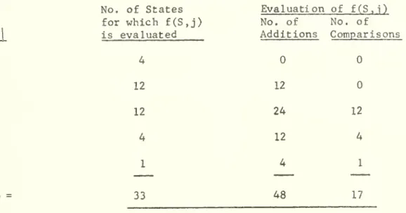
-12-TABLE II. Summary of Reduction in Both Storage and

Computational Requirements Effected by Employing Fathoming Criteria in the DP Solution of the Traveling-Salesman Example Problem.

Conventional DP Solution No. ol for wl

M

1 2 3 4 5

E

= ₃₃ 48 17 No. of States for which f(S, is evaluated

-13-This traveling -salesman example is primarily of an illustrative nature and the hybrid approach may not be

r 19 20"!

competititve with other relatively efficient algorithms i-j-^>^>-'j j-^,j. (.j^^

traveling -salesman problem. However, we are currently experimenting with

a FORTRAN IV code of the hybrid algorithm (written by Richard Kin;; of

Northwestern) and have solved the symmetric 10-city problem of -^ in

0.696 CPU seconds on a CDC 6400 with the code, fathoming 1733 of tlie

2305 possible states in the process.

The Nonlinear Knapsack Problem [32]

The nonlinear knapsack problem (NKP) can be stated as follows: N find X € IR, so as to N maximize

Z)r.(x.)

(II) j=l J J subject to N

S

g..(x.)^b.

i=l,2,...,M

j=l ^-^ J ^ X. € S j = 1,2,..., N

where (Vi) S. = [0,1,..., K.} and r.: S. -• K, is nondecr easing with

J J J J

+

r(0) = _0, (Vij)

_{g_:}

S

-

]R_^ with g. . (0)

= _{0, and b} = (h^,b^,..., b^^) > 0.

The (NKP) includes both the classical (one-dimensional) knapsack pi^blem and the multidimensional 0/1 knapsack problem as spec i i I cases.

[12J

The (NKP) also includes a number of otlic^r variants oT Llir kn.ip-Mck

roc / o 1

problem and the "optimal distribution of effort problem" ' as well

as various discrete nonlinear resource allocation problems '

g/aph-theoretic problems and nonlinear integer programming problems

-14-Consider the following (imbedded state space) dynamic programming algorithm, M&MDP 1^32]^ _{f^^ the solution of (11). Let f(n,p) denote the}

maximum objective function value of an undominated feasible solution to (11) in which at most all of the first n variables (x^,x_,..., x ) are

positive and whose resource consumption vector does not exceed

P = (^^,&2'"'' Pj^). i-e., (Vi) p.

^S

" _^ g^.(x ). For n = 1,2,..., N,

the feasible solution x = _{(Xi,x„,...,} x ) is said to be dominated by the

i z n

feasible solution x = (x,

12

,x„ x ) if we have both 2j . , r . (x .) ^

n j=l _{J J}

S

. , r.(x.) and

S

. , g, .(x .)

^S

. , g..(x.) with strict inequality J=l J J J=l ij J J=l *ij J

M

J-holding in at least one of the (M+1) inequalities. For 1 s; n s; _{N, let}

F be the (domain) set of resource consumption vectors, 3, of all un-dominated feasible solutions (x,,x„,..., x ) to the following subproblem

n max Z) r.(x.) (12) subject to ^ _n

2

g. .(x ) ^ b i = 1,2,..., M

x.€S

j=],2,...,n

Also, for ^ n ^ N, let V be the (domain) set of resource consumption vectors g (k) = _(g (k), g„ (k) ,. . . , g^ (k)), of all undominated feasible

rT^l

values of X = _{k €} S . We can demonstrate that for 1

•-2'- _n -- _N,

n n

F

nnn-1

S (V

©

F ,) with F. = _{0, where} (V

©

F ,) denotes the set obtained

U

nn-1

by forming all sums of one element of V with one element of r ,.

n n-1

Therefore, for 1 ^ n ^ N we can recursively generate all feasible candidates for F from F , and V with the following functional equation of

n n-1 n

M&MDP:

-15-with the bovindary condition f(0,0) = 0.

. (14)

If the f(n,g) corresponding to dominated solutions are

eliminated at the end of (or during) each stage n, then (13) and (14)

will yield the set of objective function values [f(N,P)| g € F } of the

complete family of undominated feasible solutions to the (NKP). Notice

that the functional equations, (13) and (14) together with the dominance elimination, are equivalent to (1) and (2) with y^ = (0,0), y = (n.p) €

^

= _{{(n,3)l 3 € F^, n} = _{0,1,..., n},} y' = _(n-1, p-g^(k)), d = k. T(y',d) =

T((n-1, e-g^(k)),k) = _(n,g) € n, {(y'.d)l T(y',d) = y] =

{ (n-l,3-g^(k)) 1

g«(^> ^ V„ ' (0-g„(k)) € F^ . , ^ b3, n(y',d) = r^(k), and k = 0.

n n n n-i n u

M6M)P is basically a one-dimensional recursive search (with dominance elimination) over the sequence of sets F ,F ,..., F which are all imbedded in the M-dimensional space B = [3|(Vi) _g^ € [0,b^]}. As

[3ll

a result of this "imbedded state space" approach , M&MDP is not

overcome by the "curse of dimensionality" which inhibits the utility of

conventional dynamic programming algorithms on higher dimensional problems. However, both the high-speed storage requirements and the computational requirements are directly related' to the length JF j of the list F of

undominated feasible solutions at stage n. Specifically, the high-speed storage requirement is on the order of (2M + 6)n where n = max (jF |} =

maximum list length and, although a very efficient dominance elimination scheme (which eliminates sorting through the use of (M+1) threaded

lists) is employed in M6WDP, the computational time tends to increase exponentially with n -- _{in fact,} problems in which n s 10,000 might con-sume hours of computer time. Fortunately, we can employ the fathoming

-16-bounds replaced by lower bounds, and vice versa) to great advantage in

reducing the list lengths.

Let ai be a lower bound on the value of an optimal solution

X € X* to the (NKP). For any (n,3) € i1, f(n,p) is the value of an

optimal solution 6' = x' = (xj , x^ ,. . . , x^ ) € A* (n,3) to subproblem

(12) for b = p. Consider the following (residual) subproblem for any

(n,3) € ^: Find (x^^,.

x^^2"-"

'^^ ^

m^^-^soas

to N max

E

r (X ) (15) j=n+l ^ ^ subject to J, J=n+1 ^^ J i = 1,2,..., M x € S j = n+1, n+2,..., N

Let X(.n,p) denote the set of all feasible solutions to

subproblem (15). Let u(n,3) be an upper bound on the value of an optimal solution to the residual subproblem (15). Then, Proposition 1.1 can be

stated for the (NKP) as follows:

PROPOSITION 2.2. (NKP) Fathoming Criterion: If for anx (n,i3) d'^l, we have

f(n,p) + l^(n,e)

<

^

(16)

then

_^

X < %(n,fci) such that x'x C X*.

•17-can be eliminated from F , thereby reducing the lengths of the lists "

k

F , F ^, ,..., F„. Since 6 € F may give rise to 11 (K. + 1) members in

" n+1 • N n

j^^^j J

list F, (n+l^TcSN) the effect of fathoming can be significant.

The choice of bounds and relaxations is dependent on the form

of both the return functions and the constraints and is discussed in detail

[281

in . The objective function value of any feasible solution to the

(NKP) provides a lower bound a£. One easily computed upper bound u(n,p)

N

for any state (n,p) €

Q

is

2

r (K.); another is min [p. (b -g )]

j=n+l J J l^i^M

where

p = max ( max {r (k)/g (k)3) (17)

n+lsij^N l^k^K -^ -^

We note that for linear problems, as a result of our solution tree structure, linear programming relaxations can be used to particular advantage. That is, in our procedure there is no backtracking and the same LP relaxation of (15) applies to all 3 € F with only the (b-g) vector changing

n

value. For fixed n the dual objective function value of any dual feasible solution of this relaxation is an upper bound for all 3 € F , allowing dual solutions to be shared.

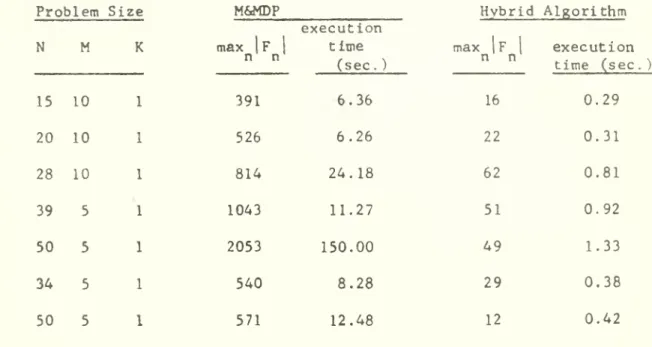
The hybrid (M&MDP witli fathoming) algorithm was coded in FORTRAN IV and applied to several of the "hard" linear problems which

[321

were solved with M6«MDP -'. The computationa] experience wiLli botli the hybrid algorithm and the straight M6.MDP arc presented in Tabic

Hi.

The times presented are the execution (CPU) times in seconds of the codes on

-18-TABLE III. Computational Comparison of the Hybrid Algorithm vs. M&MDP Problem No. 4 5 6 7 8 12 13

Problem Size M&MDP Hybrid Algorithm

N M K 15 10 20 10 28 10 39 5 50 5 34 5 50 5

-19-3. EXTENSIONS AND DISCUSSION

Our results extend immediately to dynamic programs with separable costs simply by replacing addition + with the composition

fS 29 34l

operator o ' ' whenever _it occurs. The composition operator

o

represents any cummutative isotonic binary operator, some common examples of which are addition (+), multiplication (x), and the infix

operators *- -' V and A, where _for

a^b€

IR,

aVb=

max [a,b} and

a A b = min {a,b}. Our results can also be extended to dynamic

pro-grams with general cost functions as in KARP and HELD ^ "' and _IBARAKi'- ' "'

where discrete dynamic programs are viewed as finite automata ' with

a certain cost structure superimposed upon them. That treatment allows

for the analysis of the nontrivial representation problem '- -' and requires

[33]

a somewhat different development which can be found in . In both the

separable and the general cost function extensions we assume that the

cost functions are monotone ^ ' ' ' . This is sufficient to insure that the resulting dynamic programming algorithm solves the dynamic

program.^. Furthermore, in the case of multiplicative returns ("o" = "x")

we also require that the cost functions, be normegative.

The principle ideas of this paper may be viewed as dynamic programming plus bounds (as we have done herein) or, alternatively, as

branch-and -bound plus dominance. In the latter case we could say that

node A in a branch-and-bound tree dominates node B if it can be shown that no feasible solution obtained as a descendent of B can be bctler than any optimal descendent of A. Such a strategy has proven useful

fl 2 10 21 30] on the solution of a number of problems "- » ' » » -'

. Notice that this alternative could also be broadly interpreted as using dynamic pro-gramming within a branch-and-bound framework since the dominance

elimina-tion is analogous to the initial fathoming which is employed in conventional dynamic programming.

-20-4. CONCLUSION

It has been demonstrated that both the computer storage

re-quirements and also the computational requirements of dynamic programming algorithms can be significantly reduced through the use of branch-and-bound methods. We envision that this hybrid approach may open the door-ways to the solutions of many sizes and classes of problems which are currently computationally "unsolvable" by conventional dynamic program-ming algorithms.

ACKNOWLEDGEMENTS

The authors wish to thank GEORGE NEMHAUSER and the two

21-REFERENCES

1. J. H. AHRENS and G. FINKE, "Merging and Sorting Applied to the Zero-One Knapsack Problem," Opns. Res. , forthcoming.

2. K. R. BAKER, Introduction to Sequencing and Scheduling, John Wiley

and Sons, New York, 1974.

3. R. E. BELLMAN, Dynamic Prograinrning, Princeton University Press, Princeton, N.J,, 1957.

4. and L. A. ZADEH, "Decision -Making in a Fuzzy Environment," Management Sci.

, _J7, B141 -B164 (1970).

5. M. BELI240RE and G. L. NEMHAUSER, "The Traveling-Salesman Problem: A Survey," Opns. Res. . 16, 538-558 (1968).

6. T. L. BOOTH, Sequential Machines and Automata Theory. John Wiley and

Sons, New York, N.Y., 1967.

7. N. CHRISTOFIDES, "Bounds for the Traveling-Salesman Problem," Opns.

Res..

^,1044-1056

(1972).

8. 'E. V. DENARDO and L. G. MITTEN, "Elements of Sequential Decision Processes," J. Industrial Engineering 18. 106-112 (1967).

9. V. DHARMADHIKARI, "Discrete Dynamic Programming and the Nonlinear Resource Allocation Problem." Technical Report CP-74009,

Department of Computer Science and Operations Research, Southern Methodist University, Dallas. Texas, March, 1974.

10. S. E. ELMAGHFABY, "The One-Machine Sequencing Problem with Delay

Costs," J. Industrial Engineering.

^,105-108

(1968).

11. A, 0. ESOGBUE, Personal communication, 1970.

12. B. FAALAND, "Solution of the Value-Independent Knapsack Problem by

Partitioning." Opns. Res. 2^, 333-337 (1973).

13. B. FOX, "Discrete Optimization Via Marginal Analysis," Management Sci. .

12, 210-216 (1966).

14. H. FRANK, L. T. FRISCH, R. VAN SLYKE, and W. S. CHOU, "Optimal Design

of Centralized Computer Networks," Networks 1. 43-57 (1971).

15. R. S. GARFINKEL and G. L. NEMHAUSER, Integer Programming. Wiley-Interscience, New York, N.Y., 1972.

16. A. M. GEOFFRION and R. E. MARSTEN, "Integer Programming Algorlttins

:

A Framework and State-of-the -Art-Survey," _{Management Sci} .

^,

465-491 (1972).

17. G. GRAVES and A. WHINSTON, "A Ni«w Approach to Discrete Mathonuitica1

Programming," Management Sc

L

-22-18. M, HELD and R. M. KARP, "A Dynamic Programming Approach to Sequencing Problems," J. SIAM 10. 196-210 (1962).

19. and , "The Traveling-Salesman Problem and Minimum Spanning Trees," Opns. Res.

J^, 1138-1162 (1970).

20. and , "The Traveling-Salesman Problem and Minimum Spanning Trees - Part II," Mathematical Programming 1, 6-25 (1971).

21. E. IGNALL and L. SCHRAGE, "Application of the Branch-and -Bound Technique to Some Flow-Shop Scheduling Problems," Opns. Res.

J^, 400-412 (1965). 22. T. IBARAKI, "Finite State Representations of Discrete Optimization

Problems," SIAM J. Computing 2, 193-210 (1973).

23. , "Solvable Classes of Discrete Dynamic Programming,"

J. Math. Anal, and Appl. 43, 642-693 (1973).

24. R. M. KARP and M. HELD, "Finite-State Processes and Dynamic Programming," SIAM J. Appl. Math. 15, 693-718 (1967).

25. W. KARUSH, "A General Algorithm for the Optimal Distribution of Effort," Management Sci. ^, 229-239 (1962).

26. E. L. LAWLER and D. E. WOOD, "Branch and Bound Methods: A Survey,"

Opns. Res. lA, 6.99-719 (1966).

27. J. B. MACQUEEN, "A Test for Suboptimal Actions in Markovian Decision Problems." Opns. Reg.. _J^, 559-561 (1967).

28. R, E, MARSTEN and T, L. MORIN, "A Hybrid Approach to Discrete Mathe-matical Programming," Workins Paper, Sloan School of Management,

Massachusetts Institute of Technology, Cambridge, Massachusetts, 1974.

29. L. G. MITTEN, "Composition Principles for Synthesis of Optimal Multi-stage Process," Opns. Res. U^, 610-619 (1964).

30. , "Branch-and -Bound Methods: General Formulation and Properties,"

Opns. Res . 28,24-34 (1970).

31. T. L. MORIN and A. M. 0. ESOCISUE, "Tlie Imbedded State Space A]iproach

to Reducing DimensionaliLy Lii Dynamic Programs ol ili;;hur

Dimen-sions," J. Math. Anal, and Appl. 48, 801-810 (1974).

32. and R. E. MARSTEN, "An Algorithm for Nonlinear Knapsack Problems," Technical Report No. _95^, Operations Research Center, Massachusetts Institute of Tccl-ii-ioTogy, Cambridge, Massachusetts,

May, 1974, to appear in Management Sci.

33. and , "Branch-and -Bound Strategies for Dynamic

Programming," Discussion Paper No. 106, The Center For MaLhcniatical Studies in Economics and Management Science, Northwestern University,

-23-34. G, L. NEMHAUSER, Introduction to Dynamic Programming. John Wiley and Sons, New York, N.Y., 1966.

35. . , "A Generalized Permanent Label Setting Algorithm for the Shortest Path Between Specified Nodes," J. Math. Anal, and Appl. 38, 328-334 (1972).

36. E. L. PORTEUS, "Some Bounds for Discounted Sequential Decision Processes," Management Sci. 18, 7-11 (1971).

37. F. PROSCHAN and T. A. BRAY, "Optimal Redundancy Under Multiple Con-straints," Opns. Res. 13, 800-814 (1965).

38. M. D. RABIN and D. SCOTT, "Finite Automata and their Decision Problems," IBM J. Res. and Development 3. 114-125 (1959).

39. H. M. SALKIN and C. A. DE KLUYVER, "The Knapsack Problem:

A

Survey," Technical Memorandum No. 281, Department of Operations Research, Case Western Reserve University, Cleveland, Ohio, December, 1972. 40. R. E. SCHWARTZ and C. L. DYM, "An Integer Maximization Problem,"

Opns. Res. IS, 548-550 (1971).

41. 'R. VAN SLYKE and A. KERSHENBAUM, "Network Analysis by Accumulation of Trees," Lecture Notes for the course, Mathematical Programming for

Management Decision: Theory and Application, Massachusetts

•.,, Institute of Technology, Cambridge, Massachusetts, July, 1973.

42. H. M. WAGNER, Principles of Operations Research. Prentice-Hall, Englewood Cliffs, N.J., 1969.

43. H. M. WEINGARTNER and D. N. NESS, "Methods for the Solution of the Multi-Dimensional 0/1 Knapsack Problem," Opns. Res. _J^, 83-103

Date

Due

ST

>'\i\ .9^ Auez-vatt. ^EEA^'

JUK

2 9 1^83 JAM :::> MAR,

2

.: t' • . Lib-26-67

III|II1IM||JI|||I|I| 3 TQflD DO MriLI_BRflftIFS

l-il-yH

3

b71

fl7T HD28.M414 no.748- 74

Kearl, James R/Relationships between t 7316155, P»BKSD»BK 0003771

|iliiimill ! iii:i|iii IIIiii|i|iiiii|iliTiiiiliii

llil J Li. LllJiiillI..Jilllill

M^TIIbRAftif..

firr

3 "iDflO 000 flbb ??T 3 TOfiD

ODM

qfl3

^^^

I'-f'/'V-l 3 TDflD

_{DD3 70^}

_^4a

7?0cu--7V

75c

-7if 3 TOflD

_{DD3 b?l TtD}

MilLiBHARlES 3 TDflD

DD3

71 b 1

'j£4-7i

3

'Oao 003 702

5 MIT LIBRARIES

07

3 TDflD

DD3 b71 754

1SZ

153-7^